Fluctuation induced interactions between domains in membranes

Abstract

We study a model lipid bilayer composed of a mixture of two incompatible lipid types which have a natural tendency to segregate in the absence of membrane fluctuations. The membrane is mechanically characterized by a local bending rigidity $\kappa(\phi)$ which varies with the average local lipid composition $\phi$. We show, in the case where $\kappa$ varies weakly with $\phi$, that the effective interaction between lipids of the same type can either be everywhere attractive or can have a repulsive component at intermediate distances greater than the typical lipid size. When this interaction has a repulsive component, it can prevent macro-phase separation and lead to separation in mesophases with a finite domain size. This effect could be relevant to certain experimental and numerical observations of mesoscopic domains in such systems.

I Introduction

At the simplest level biological membranes are modeled by homogeneous flexible bilayers of amphiphilic lipid molecules hel ; seifert . However, in many physical and biological situations, these membranes are inhomogeneous on some microscopic scale. Indeed four major distinct lipid types are typically present in mammalian cell membranes alberts . It is natural to ask what may be the role of this homogeneity in the biological context and how it influences the mechanical properties of the cell. The interplay between the lipid composition and membrane fluctuations has been addressed in many recent studies. The local composition of the membrane will clearly affect its fluctuations and local geometry. Indeed, the coupling between membrane fluctuations and local composition is at the origin of the budding instability lip ; juli seen in certain systems. On the other hand, membrane fluctuations will also influence its local composition. In this paper we will examine how the coupling of membrane fluctuations to local composition can affect the phase ordering of its component lipids.

In previous works, the way in which the fluctuation–composition coupling is incorporated into the overall free energy of system falls into two main classes: i) The membrane is composed of a homogeneous lipid background with added insertions such as trans-membrane proteins and attached polymers. ii) The membrane is modeled as a multicomponent system with several lipid types and where the mechanical properties of the system are dependent on the relative local concentrations of the various lipid types.

The insertions considered in models of class i) modify the membrane fluctuations via several different mechanisms. First point-like inclusions, such as polymers, exert a pressure distribution on the flexible membrane. This involves a coupling of the membrane composition, in this case the density field of the inclusions, to the height $h({\bf x})$ over the projected area of the membrane. Another possible coupling is via an imposed boundary condition on the height field $h$ at the boundary between the inclusions and the membrane. For example, the contact angle at the boundary can be taken to be fixed in order to minimize the hydrophobic free energy of the insertion. This is an example of a hard constraint. Alternatively one can introduce a general coupling tensor, related to the orientational degrees of freedom of the inclusions, to the local strain tensor $\nabla_{i}\nabla_{j}h$, from which the curvature tensor can be extracted. This then corresponds to an energetic term which induces a preferred local curvature. In the literature several types of inclusions are considered: circular gobrpi1 ; gou1 ; kineos , elliptic palu , more general dofo1 ; dofo2 ; misbah1 ; barfo embedded inclusions, as well as adsorbed cylinders gol . Besides introducing a tendency for a spontaneous local curvature, which breaks the up-down symmetry of the system, inclusions may also modify the energy associated wit terms quadratic in the curvature tensor. For example isotropic inclusions may modify the local bending and Gaussian rigidities of the membrane. In the case of two inclusions one may then explicitly evaluate their effective interaction. To summarize, the density field of the inclusions in all these cases is coupled via: (a) $h$ in the case of insertions exerting a pressure, (b) an effective vectorial $\nabla_{i}h$ coupling in the case of imposed boundary conditions at the inclusions frontier with the membrane, (c) a two tensor coupling to $\nabla_{i}\nabla_{j}h$ when there is a locally preferred curvature tensor and finally (d) a coupling to $\nabla_{i}\nabla_{j}h\nabla_{k}\nabla_{l}h$, when the local bending and Gaussian rigidities are modified by the inclusions and also when non-isotropic effects are present. The above are the most physically relevant couplings up to quadratic order and consequently are the most significant in systems where the height fluctuations are relatively small.

In this case of models of type ii), the variation of the elastic properties of the membrane is more continuous than in the case of inclusions. If one neglects the possibility of non-isotropic effects, the most natural parameters which will vary with local lipid composition are the bending rigidity $\kappa$, the Gaussian rigidity $\overline{\kappa}$ and the spontaneous local curvature $c$. For instance a concentration dependent spontaneous curvature is considered in leibler ; tani ; saxena ; misbah2 . Linear perturbations to both the bending rigidity and the spontaneous curvature are studied in netz ; nepi . In gobrpi1 , linear perturbations to the bending and Gaussian rigidity were considered, the interaction arising in this case is proportional to $1/r^{4}$ and the prefactor is given by the product of coefficients of the linear deviations from the average value of $\kappa$ and $\overline{\kappa}$. The induced interaction may thus be attractive or repulsive depending on the sign of these coefficients. Of course models of type (i), with discrete inclusions, can be described by models of type (ii) when it makes sense to take a continuum limit for the inclusions. This limit will be valid for inclusion sizes which are comparable to the microscopic length scale of the membrane, that is to say the lateral lipid size.

All of the studies mentioned above assume zero surface tension. However, the study of membranes under tension sheds light upon the physics of biological membranes which are not truly at equilibrium but under external constraints or perturbations. The surface tension can be due to electrostatic interactions with the aqueous solvent or due to the presence of molecular protrusions. Furthermore, the external action of laser tweezers on a vesicle attracts phospholipids an puts the membrane under tension. This leads to interesting phenomena such as pearling instabilities barziv . It has been theoretically shown that the presence of surface tension can induced a repulsive interaction between inclusions of the same type sens ; sens2 . The model used in sens ; sens2 is of type i) and is based on a linear coupling of the inclusion to the height of the membrane, for example to model the local pressure exerted by an attached polymer. The interaction is sensitive to the strength of membrane-inclusion coupling. In this system, the up-down symmetry of the membrane is clearly broken by the linear coupling. Indeed, in many biological situations the up-down symmetry of the membrane is clearly broken for instance by different compositions in the top and bottom leaves or by the presence of conical trans-membrane inclusions. However, it is interesting to ask if the presence of surface tension can also lead to repulsive interaction between domains, with similar lipid composition, even when the up-down symmetry is conserved.

The physics of phase separation may play an important role in biological systems. It has been experimentally shown that erythrocyte membranes which contain many different lipid types form immiscible two dimensional liquids, which are very close to the miscibility critical point keller . The resulting thermodynamic forces can affect the mechanical properties of the membrane and in particular its shape. However, in turn the fluctuations will also affect the distribution of the components in the membrane. As an example, a long-range fluctuation mediated repulsion between inclusions, combined with a short-range van der Waals attraction, could lead to the formation of mesoscopic domains tani ; sear of the inclusions. It has also been shown that the presence of a surface tension modifies the effective interactions between conical inclusions wkh , inclusions of the same type are always repelled but oppositely orientated inclusions interact attractively at long distances and then repel at shorter distances. This is in contrast to the case where there is no tension when all interactions are always repulsive.

In this paper, we consider a two-component bilayer with the up-down symmetry and, in general, with a non-zero surface tension. We show that for certain variations of the bending rigidity and the local surface energy (the composition independent component of which can be interpreted as a surface tension) with the local composition in lipids, a fluctuation induced lipid-lipid repulsive interaction can appear between domains of similar composition. This, together with a short-range van der Waals attraction, can induce the formation of mesophases. In the scheme of previous models, our model falls into the class of type ii) above and our cumulant expansion method is similar to that used in gobrpi1 and netz ; nepi . In our study we add an non-zero surface energy, as in  sens ; sens2 , but where this local surface energy fluctuates with the local lipid composition.

The paper is organized as follows. In Section II we present our field theoretical model. In section III using a cumulant expansion for small height fluctuations we calculate the induced interaction, this rather technical section may be skipped by a reader interested only in the physical consequences of the calculation. In section IV the general physical properties and asymptotic behavior of this effective interaction are discussed. Section V is devoted to a description of the results which are compared to previous studies. In addition we suggest a possible experiment where the effects predicted here could possibly be seen.

II Field-theoretical formulation

We consider a model membrane with two lipid types $A$ and $B$ and where the top and bottom leaves have the same lipid composition. In the most frequent case, at least whenever van der Waals interactions are dominant, it is energetically favorable for lipids of the same type to be adjacent. In this case, we can write down a typical attractive energy per site $E=\chi\phi_{A}\phi_{B}$ where $\phi_{A}$ and $\phi_{B}$ are the liquid volume fraction of lipid $A$ and $B$ and $\chi>0$ is a Flory parameter related to electronic polarizabilities of both molecules. We will consider a coarse-grained model for a field $\phi$ related to the local surface fraction of the two lipid types, i.e. $\phi=\phi_{A}-\phi_{B}$, which in the absence of surface fluctuations exhibits a continuous phase transition at sufficiently low temperatures. The theory is then described by the Ginzburg-Landau Hamiltonian tani

$$H^{I}[\phi]=\int\sqrt{g}d^{2}{\bf x}\ \left[{J\over 2}g^{ij}\nabla_{i}\phi\nabla_{j}\phi+V(\phi)\right],$$ (1)

which is written in a covariant form which ensures the independence of the energy from the choice of the two dimensional coordinate system denoted by ${\bf x}$. The parameter $J$ is positive and related to the Flory parameter $\chi$, it is a ferromagnetic interaction and energetically favors lipids of the same type being next to each other. The potential $V(\phi)$ fixes the two characteristic values of $\phi$ and the global composition via chemical potential like terms. As the potential $V$ appears in $H$ simply integrated over the area of the membrane, it can be interpreted as a composition dependent contribution to the surface energy of the membrane. Indeed, the constant part of $V$ which is $V(0)$ can be interpreted as a surface tension because it is coupled to the total physical area of the membrane $\int\sqrt{g}d^{2}{\bf x}$. The term $V(0)$ can thus be used as a Lagrange multiplier to fix the physical membrane area. As mentioned above, $V$ will have a $\phi$ dependence as in the usual Landau models for phase separating systems. As in standard Landau theory, we will assume that $V$ is a single well at high temperature and a double well at low temperature. This means that the system on a plane will exhibit a continuous phase transition. At the mean field level, this transition occurs when when the mass associated to this field theory, given by $M^{2}_{0}=V^{\prime\prime}(\phi_{0})$, vanishes (where $\phi_{0}$ is the homogeneous mean field solution). This transition exhibits a divergent correlation length and corresponds to a macro-phase separation which occurs at a critical temperature $T=T_{c}$.

In the above, the metric of the membrane surface is denoted by $g_{ij}$ and in the Monge gauge it is given by

$$g_{ij}=\delta_{ij}+\nabla_{i}h\nabla_{j}h$$ (2)

where $h$ is the height of the surface above the projection plane whose area we will denote by $A$. The term $g$ denotes the determinant of $g_{ij}$ and is given by

$$g=1+(\nabla h)^{2}.$$ (3)

Hence the Hamiltonian given by Eq. (1) already implicitly includes a coupling between the local composition, as encoded by $\phi$, and the membrane fluctuations, as encoded by $h$. The interface energy or line tension, which corresponds to the term quadratic in the gradient, is written as to ensure covariance; $g^{ij}$ is the inverse of $g_{ij}$ and is given by

$$g^{ij}=\delta^{ij}-{\nabla_{i}h\nabla_{j}h\over 1+(\nabla h)^{2}}.$$ (4)

Here we note that the fact that one should use the covariant form of the line tension is often forgotten in the literature. To lowest, i.e. quadratic order in the fluctuations $h$, one has

$$H^{I}[\phi,h]=\int d^{2}{\bf x}\ \left[{J\over 2}(\nabla\phi)^{2}+V(\phi)\right]+\int d^{2}{\bf x}\ \left[{J\over 4}(\nabla\phi)^{2}(\nabla h)^{2}-{J\over 2}(\nabla\phi\cdot\nabla h)^{2}+{1\over 2}(\nabla h)^{2}V(\phi)\right]$$ (5)

We now take into account the elastic energy of the membrane so the total Hamiltonian of the system is given by

$${\cal H}[\phi,h]=H^{I}[\phi,h]+H^{S}[\phi,h].$$ (6)

The Hamiltonian for surface fluctuations will be taken to be

$$H^{S}[\phi,h]={1\over 2}\int d^{2}{\bf x}\ \kappa(\phi)\left(\nabla^{2}h\right)^{2}$$ (7)

which is the simplest Helfrich Hamiltonian for surface fluctuations hel and correspond, strictly speaking, to the first term in an $\nabla^{2}h$-expansion of the mean curvature seifert . This Hamiltonian corresponds to a bending energy with local bending rigidity which depends on the local composition characterized by $\phi$. The two dimensional membrane system is assumed to have no spontaneous curvature and thus has an up-down symmetry. More generally, one could also include a composition dependence on the Gaussian rigidity, the contribution coming from this term would then cease to be a topological invariant and should strictly be included.

The effective partition function in the presence of membrane fluctuations is given by

$$Z=\int d[\phi]d[h]\exp(-\beta{\cal H})$$ (8)

where $\beta^{-1}=k_{B}T$ is the thermal energy scale. We recall that $A$ is the projected area of the membrane, the physical area of the membrane is denoted by $A+\Delta A$, where $\Delta A$ is often called the excess area. For typical biological membranes, $\Delta A/A$ is small, of the order of a few percent, and we will thus legitimately assume, in the rest of the paper, that height fluctuations are small compared to the typical length scale of the system.

III Calculation of the fluctuation induced interaction

In this section we explicitly calculate the fluctuation induced interaction to second order in the cumulant expansion.

In the high temperature regime, lipids form a mixed phase characterized by a homogeneous and uniform composition $\phi_{0}$, with fluctuations $\psi$ about $\phi_{0}$. In an ensemble where the average value of $\phi$ is fixed write $\phi=\phi_{0}+\psi$ where $\phi_{0}=A^{-1}\int d^{2}{\bf x}\,\phi({\bf x})$. Consequently in this case, we have $\int d^{2}{\bf x}\,\psi({\bf x})=0$. By assuming that $\kappa$ and $V$ behave continuously around $\phi_{0}$, we expand the total Hamiltonian (6) up to $\mathcal{O}(\psi^{2})$ in the fluctuations. This leads to

$${\cal H}[\phi_{0},\psi,h] = AV(\phi_{0})+H^{I}_{0}[\phi_{0},\psi]+H^{S}_{0}[\phi_{0},h]+\Delta H[\phi_{0},\psi,h],$$ (9)

$$H^{I}_{0}[\psi] = \frac{1}{2}\int d^{2}{\bf x}\ \left[J(\nabla\psi)^{2}+V^{\prime\prime}(\phi_{0})\psi^{2}\right],$$ (10)

$$H^{S}_{0}[h] = \frac{1}{2}\int d^{2}{\bf x}\ \left[\kappa(\phi_{0})\left(\nabla^{2}h\right)^{2}+V(\phi_{0})\left(\nabla h\right)^{2}\right].$$ (11)

When the term proportional to $V(\phi_{0})$ is included in the surface Hamiltonian $H_{0}^{S}$, as we have chosen to do above, $V(\phi_{0})$ can be interpreted as an effective elastic energy. However, because it is constant, $V(\phi_{0})$ can be interpreted as an effective surface tension. The part of the Hamiltonian which we will treat perturbatively is

$$\Delta H[\phi_{0},\psi,h] = \frac{1}{2}\int d^{2}{\bf x}\ \left\{J\left[{1\over 2}(\nabla\psi)^{2}(\nabla h)^{2}-(\nabla\psi\cdot\nabla h)^{2}\right]+\left[V^{\prime}(\phi_{0})(\nabla h)^{2}+\kappa^{\prime}(\phi_{0})(\nabla^{2}h)^{2}\right]\psi\right.$$ (12)

$$+ \left.\frac{1}{2}\left[V^{\prime\prime}(\phi_{0})(\nabla h)^{2}+\kappa^{\prime\prime}(\phi_{0})(\nabla^{2}h)^{2}\right]\psi^{2}\right\}.$$

The scheme of the calculation is just slightly different in the case where the value of $\phi_{0}$ is allowed to fluctuate but nothing intrinsically changes.

We perform a cumulant expansion in the partition function (8) as follows

$$Z \approx Z^{S}_{0}\exp(-\beta AV(\phi_{0}))\int d[\psi]\exp(-\beta H^{I}_{0})\left[1-\beta\langle\Delta H\rangle^{S}+\frac{\beta^{2}}{2}\langle(\Delta H)^{2}\rangle^{S}\right]$$ (13)

$$\approx \int Z^{S}_{0}\exp(-\beta AV(\phi_{0}))\int d[\psi]\exp\left(-\beta{\cal H}_{\mathrm{eff}}[\phi_{0},\psi]\right)$$ (14)

where $Z^{S}_{0}=\int d[h]\exp(-\beta H^{S}_{0})$ and $\langle\mathcal{O}\rangle^{S}=(Z^{S}_{0})^{-1}\int d[h]\mathcal{O}\exp(-\beta H^{S}_{0})$. The cumulant expansion at this order is clearly exact to $\mathcal{O}(\psi^{2})$. The effective interaction at this order is thus given by

$${\cal H}_{\mathrm{eff}}[\phi_{0},\psi]=H_{0}^{I}[\phi_{0},\psi]+\langle\Delta H\rangle^{S}_{c}-\frac{\beta}{2}\langle(\Delta H)^{2}\rangle^{S}_{c}$$ (15)

where the subscript $c$ indicates that it is the connected part of the correlation function.

Note that only the first term in the cumulant expansion can lead to a quadratic terms in $\nabla\psi$, however this term can be seen to be zero by the following:

$$\langle\frac{1}{2}(\nabla\psi)^{2}(\nabla h)^{2}-(\nabla\psi\cdot\nabla h)^{2}\rangle^{S}_{c} = \frac{1}{2}(\nabla\psi)^{2}\langle(\nabla h)^{2}\rangle^{S}_{c}-\nabla_{i}\psi\nabla_{j}\psi\langle\nabla_{i}h\nabla_{j}h\rangle^{S}_{c}$$ (16)

$$= \frac{1}{2}(\nabla\psi)^{2}\langle(\nabla h)^{2}\rangle^{S}_{c}-\nabla_{i}\psi\nabla_{j}\psi\ \delta_{ij}\ \frac{1}{2}\langle(\nabla h)^{2}\rangle^{S}_{c}=0,$$

where we have appealed to the isotropy of the system. There is therefore no renormalization of the coupling $J$. Also in the first term of the cumulant expansion, terms linear in $\psi$ cancel by definition of $\psi$ (as they are integrated against a constant by isotropy) and the remaining terms yield $\langle\Delta H\rangle^{S}_{c}=\frac{1}{2}\int d^{2}{\bf x}M_{1}^{2}\psi^{2}$ where the mass $M_{1}$ is given by

$$M_{1}^{2}=\frac{1}{2}\left[V^{\prime\prime}(\phi_{0})\langle(\nabla h)^{2}\rangle^{S}_{c}+\kappa^{\prime\prime}(\phi_{0})\langle(\nabla^{2}h)^{2}\rangle^{S}_{c}\right].$$ (17)

Again to quadratic order in $\psi$, the second order term in the cumulant expansion yields

$$-\frac{\beta}{2}\langle(\Delta H)^{2}\rangle^{S}_{c}=\frac{1}{2}\int d^{2}{\bf x}d^{2}{\bf y}\psi({\bf x})U({\bf x}-{\bf y})\psi({\bf y})$$ (18)

where

$$U({\bf x}-{\bf y})=-{\beta\over 4}\left[{\kappa^{\prime}}^{2}(\phi_{0})\langle\left(\nabla^{2}h({\bf x})\right)^{2}\left(\nabla^{2}h({\bf y})\right)^{2}\rangle^{S}_{c}+2V^{\prime}(\phi_{0})\kappa^{\prime}(\phi_{0})\langle\left(\nabla^{2}h({\bf x})\right)^{2}\left(\nabla h({\bf y})\right)^{2}\rangle^{S}_{c}+{V^{\prime}}^{2}(\phi_{0})\langle\left(\nabla h({\bf x})\right)^{2}\left(\nabla h({\bf y})\right)^{2}\rangle^{S}_{c}\right].$$ (19)

The potential $U({\bf x}-{\bf y})$ is non-local and characterizes the induced interaction mediated by height fluctuations. The various connected correlation functions above are evaluated as

$$\left\langle(\nabla^{2}h({\bf x}))^{2}(\nabla^{2}h({\bf y}))^{2}\right\rangle_{c}^{S} = {2\over\beta^{2}}(\nabla^{4}G({\bf x}-{\bf y}))^{2}$$

$$\left\langle(\nabla h({\bf x}))^{2}(\nabla h({\bf y}))^{2}\right\rangle_{c}^{S} = {2\over\beta^{2}}\sum_{ij}(\nabla_{i}\nabla_{j}G({\bf x}-{\bf y}))^{2}$$

$$\left\langle(\nabla^{2}h({\bf x}))^{2}(\nabla h({\bf y}))^{2}\right\rangle_{c}^{S} = {2\over\beta^{2}}(\nabla\nabla^{2}G({\bf x}-{\bf y}))^{2}.$$ (20)

Here the Green function $G$ is given by

$$G=(\kappa(\phi_{0})\nabla^{4}-V(\phi_{0})\nabla^{2})^{-1}={1\over V(\phi_{0})}(G_{0}-G_{m}),$$ (21)

where

$$\xi=\frac{1}{m}=\sqrt{\frac{\kappa(\phi_{0})}{V(\phi_{0})}}.$$ (22)

The intrinsic length $\xi$ is usually in the range 10–100 nm for biological membranes. The Green function $G_{0}$ is $G_{0}=-\frac{1}{2\pi}\ln\left|\frac{\bf x}{L}\right|$ ($L$ is an arbitrary length) and $G_{m}$ is the Yukawa interaction given by

$$-\nabla^{2}G_{(}{\bf x})+m^{2}G_{m}({\bf x})=\delta({\bf x}).$$ (23)

In two dimensions one has

$$G_{m}({\bf x})=\frac{1}{2\pi}K_{0}(m|{\bf x}|),$$ (24)

where $K_{0}(x)$ is the Bessel function of the second kind of order 0. Using these results we find that

$$U({\bf x})=B\delta({\bf x})+v(|{\bf x}|).$$ (25)

The first term of the r.h.s. is short-ranged with $B=-(m^{4}/2\beta)[\kappa^{\prime}(\phi_{0})/\kappa(\phi_{0})]^{2}[\delta(0)-2m^{2}G_{m}(0)]$ and needs to be regularized via an ultra-violet cut-off $\Lambda=2\pi/a$ corresponding to a microscopic length scale $a$ which would be of the order of the distance between lipid heads. The second term $v$ of the r.h.s. above is the long-range induced interaction and is independent of the ultra-violet cut-off. It is given by

$$v(r) = \frac{m^{4}}{2\beta}\left[\frac{\kappa^{\prime}(\phi_{0})}{\kappa(\phi_{0})}\right]^{2}\nu_{\alpha}(u),$$ (26)

$$\nu_{\alpha}(u) = -\frac{1}{4\pi^{2}}\left\{K_{0}^{2}(u)+2\alpha K^{\prime 2}_{0}(u)+\alpha^{2}\left[\left(K^{\prime\prime}_{0}(u)-{1\over u^{2}}\right)^{2}+{1\over u^{2}}\left(K^{\prime}_{0}(u)+{1\over u}\right)^{2}\right]\right\}$$ (27)

where $u=m|{\bf x}|=mr$ and

$$\alpha=\frac{V^{\prime}(\phi_{0})}{V(\phi_{0})}\frac{\kappa(\phi_{0})}{\kappa^{\prime}(\phi_{0})}.$$ (28)

IV Properties of the fluctuation induced interaction

Here we discuss the features of the interaction derived in section III. First, the strength of this interaction is polynomial in $m$ and therefore reducing the local surface or elastic energy and increasing the local bending rigidity reduces considerably the interaction energy. This same reduction however also increases the range of the interaction. Secondly, the interaction strength is set by $k_{B}T$, which means that this interaction has an entropic origin.

If $\alpha$ is positive, we see that the interaction between areas having the same lipid type (with the same sign of $\psi$) is always attractive. To see this, we note that in the expression for $v(u)$, Eq. (26), the coefficients of $\alpha^{0}$, $\alpha$ and $\alpha^{2}$ are functions of $u$ which are positive and monotonically decreasing hence yielding an attractive interaction at all distances. In a ferromagnetic analogy where the lipid types are characterized by a field $\phi$ having the values concentrated about $\pm 1$, this corresponds to a long-range ferromagnetic interaction which enhances the short-range one already present. However when $\alpha$ is negative, $v$ now has a repulsive component, corresponding to the coefficient of $\alpha$, which could prevent macro-phase separation.

For large $u$ we have abram

$$K_{0}(u)\approx\sqrt{\frac{\pi}{2u}}\exp(-u)$$ (29)

and thus at large distances $v$ behaves as

$$v(r)\approx-\frac{k_{B}T}{4\pi^{2}}\left[\frac{V^{\prime}(\phi_{0})}{V(\phi_{0})}\right]^{2}\frac{1}{r^{4}}.$$ (30)

This $1/r^{4}$ interaction, which is always attractive, is typically seen between inclusions of the same type in membranes without surface tension and is found in many of the studies discussed in the Introduction. However, this $1/r^{4}$ attraction does not have the the same physical origin as in previous studies because, as can be seen by examining the prefactor, it is generated solely by the fluctuations of the surface energy.

For small $r$ we find

$$v(r)\approx-\alpha\frac{k_{B}T}{8\pi^{2}}\left[\frac{\kappa^{\prime}(\phi_{0})}{\kappa(\phi_{0})}\right]^{2}\frac{m^{2}}{r^{2}}+\mathcal{O}(\ln^{2}r)\approx-\frac{k_{B}T}{4\pi^{2}}\frac{\kappa^{\prime}(\phi_{0})V^{\prime}(\phi_{0})}{\kappa^{2}(\phi_{0})}\frac{1}{r^{2}}+\mathcal{O}(\ln^{2}r)$$ (31)

which is again attractive if $\alpha>0$ but is repulsive when $\alpha<0$ (or $\kappa^{\prime}(\phi_{0})V^{\prime}(\phi_{0})<0$). In this last case, the overall interaction is somewhat frustrated: it is attractive at very short length scales (of the order of the microscopic length scale) due to van der Waals interactions (in our model represented by the local ferromagnetic interaction), together with a longer range membrane mediated repulsion over intermediate length scales, before becoming attractive at longer length scales. One can can suppose that the occurrence of these attractive and repulsive interactions can prevent macroscopic phase separation and lead to mesoscopic domains.

V Microphase separation

The final effective quadratic Hamiltonian can now be written as

$${\cal H}_{\mathrm{eff}}[\phi_{0},\psi]=\frac{1}{2}\int d^{2}{\bf x}\ \left[J(\nabla\psi)^{2}+M_{2}^{2}\psi^{2}\right]+\frac{1}{2}\int d^{2}{\bf x}d^{2}{\bf y}\psi({\bf x})v({\bf x}-{\bf y})\psi({\bf y}),$$ (32)

where the corrected mass is given by $M_{2}^{2}=M_{0}^{2}+M_{1}^{2}+B$. It is important to note that this mass depends on the microscopic cutoff $a$ since $M_{1}^{2}$ includes the expectation values $\langle(\nabla^{2}h)^{2}\rangle^{S}$ and $\langle(\nabla h)^{2}\rangle^{S}$ which diverge and must thus be regularized and a similar regularization is needed to evaluate $B$. As already explained in the Introduction, we consider systems such that, in the absence of height fluctuations, when $M_{0}\to 0$ the system exhibits a second order phase transition with diverging correlation length $\ell_{0}=\sqrt{J}/M_{0}$. In Fourier space, we find

$${\cal H}_{\mathrm{eff}}[\phi_{0},\psi]={1\over 2(2\pi)^{2}}\int d^{2}{\bf q}\left[Jq^{2}+M_{e}^{2}+w(q)\right]{\tilde{\psi}}({\bf q}){\tilde{\psi}}({\bf-q}),$$ (33)

where $q=|{\bf q}|$ and the Fourier transform and its inverse are defined by

$$f({\bf x}) = \int\frac{d^{2}{\bf q}}{(2\pi)^{2}}{\tilde{f}}({\bf q})\exp(i{\bf q}\cdot{\bf x}),$$ (34)

$${\tilde{f}}({\bf q}) = \int d^{2}{\bf x}f({\bf x})\exp(-i{\bf q}\cdot{\bf x}).$$ (35)

In the Fourier representation the non-local part of the interaction is given by $w(q)={\tilde{v}}(q)-{\tilde{v}}(0)$ and $M_{e}^{2}=M^{2}_{2}+{\tilde{v}}(0)$ thus gives effective mass for the theory.

The stability of the homogeneous solution against phase separation is determined by the lipid-lipid correlation function in Fourier space $\langle{\tilde{\psi}}({\bf q}){\tilde{\psi}}({\bf q}^{\prime})\rangle=(2\pi)^{2}\delta({\bf q}+{\bf q}^{\prime})S({\bf q})$ where the structure factor is

$$S({\bf q})=\frac{k_{B}T}{Jq^{2}+M^{2}_{e}+w(q)}$$ (36)

Defining

$$\epsilon=\left[\frac{\kappa(\phi_{0})}{\kappa^{\prime}(\phi_{0})}\right]^{2},$$ (37)

we find three dimensionless parameters in the structure factor

$${\tilde{S}}({\tilde{q}})=\frac{S({\tilde{q}})}{2\epsilon\xi^{2}}=\frac{1}{2\epsilon\beta J\left[(\xi/\ell_{e})^{2}+{\tilde{q}}^{2}\right]+W_{\alpha}({\tilde{q}})}$$ (38)

where ${\tilde{q}}=\xi q$, which are $\alpha$, $\epsilon\beta J$ and $\ell_{e}^{2}=J/M^{2}_{e}$. The Fourier transform of the dimensionless potential is

$$W_{\alpha}({\tilde{q}})=2\pi\int_{0}^{\infty}udu\left[J_{0}({\tilde{q}}u)-1\right]\nu_{\alpha}(u),$$ (39)

where $J_{0}(x)$ is the Bessel function of the first kind of order 0. A divergence of the structure factor, Eq. (38) at ${\tilde{q}}=0$, while $S$ remains finite for ${\tilde{q}}\neq 0$ signals a macro-phase separation. In this case, since we find $S(0)=\ell_{e}^{2}/(\beta J)$, the phase separation occurs when the correlation length $\ell_{e}\to\infty$ and this corresponds to the case where the induced interaction does not change the nature of the transition but only changes where it occurs. We show the behavior of $W_{\alpha}({\tilde{q}})$ and ${\tilde{S}}({\tilde{q}})$ for different values of $\alpha$ in Fig 1. When $\alpha\geq 0$, $W_{\alpha}(q)$ and its first derivative are always positive, and the only maximum of the structure factor occurs at ${\tilde{q}}=0$.

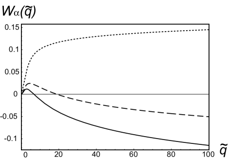
Figure 1: Plot of $W_{\alpha}({\tilde{q}})$ for various values of $\alpha$: $0.05$ (dotted line), $-0.1$ (broken line) and $-0.15$ (solid line).

However, when $\alpha<0$ we see that for particular values of $\epsilon\beta J$ and $\xi/\ell_{e}$, ${\tilde{S}}({\tilde{q}})$ reaches a maximum at an intermediate values of ${\tilde{q}}$ and this maximum can even diverge at a non-zero wave-vector ${\tilde{q}}^{*}$. In this case, the homogeneous solution becomes unstable before $\ell_{e}\to\infty$ which leads to the formation of mesophases (mesoscopic phase separation) with a finite characteristic length scale given by $\xi/{\tilde{q}}^{*}$. Note that at large values of ${\tilde{q}}$, we have $W_{\alpha}({\tilde{q}})\sim\alpha\ln{\tilde{q}}$ but this short-range component of the induced interaction is dominated by the short-range van der Waals interaction term whose strength is controlled by $J$, and $S({\tilde{q}})$ ultimately decreases as $1/{\tilde{q}}^{2}$ for large ${\tilde{q}}$. The maximum of the structure factor diverges for an intermediate wave-vector ${\tilde{q}}^{*}$ which is implicitly defined by the two following equalities

$$W^{\prime}_{\alpha}({\tilde{q}}^{*})+4\epsilon\beta J{\tilde{q}}^{*} = 0$$ (40)

$$W_{\alpha}({\tilde{q}}^{*})+2\epsilon\beta J\left[{\tilde{q}}^{*2}+(\xi/\ell_{e})^{2}\right] = 0$$ (41)

i.e. when the parabola $-2\epsilon\beta J[{\tilde{q}}^{2}+(\xi/\ell_{e})^{2}]$ is tangent to $W_{\alpha}({\tilde{q}})$. Given the number of parameters in our theory the evaluation of a complete phase diagram is unfeasible, however the  fundamental question we wish to address is whether there is a macro-phase or micro-phase separation. To do this we can examine the structure factor at the point where the ${\bf q}=0$ mode becomes unstable, that is to say where the effective mass $M_{e}=0$. This is thus equivalent to examining temperatures $T_{c}$ which are critical in the true sense. If the modes ${\bf q}\neq 0$ are stable at $T_{c}$ then we expect to see the macro-phase separation. However if at $T_{c}$ there is already a mode $q\neq 0$ which is unstable then a micro-phase separation must have already occurred at a temperature $T>T_{c}$. Thus, without having to specify the full theory, we can identify when a macro-phase separation is converted to a micro-phase one due to coupling between membrane fluctuations and its composition.

Since we are interested in the behavior of the structure factor when approaching the macro-phase transition ($\ell_{e}\to\infty$); we calculate the onset of the micro-phase separation given by Eqs. (40)–(41) for $\xi/\ell_{e}=0$ i.e. at the critical temperature $T_{c}$. The result is shown in Fig. 2: the gray region corresponds to the region of the phase diagram ($\epsilon\beta J$, $\alpha$) where mesophases appears whereas the white region corresponds to macro phase separation. The solid line corresponds to the solution of Eqs. (40)–(41) (the dots are the exact solutions). This ”phase diagram” is plotted at a fixed lipid composition $\phi_{0}$ and fixed temperature $T=T_{c}$ corresponding to the critical point in the ($\phi$, $T$) space. It is important to note that when the temperature deviates from the critical temperature, the correlation length $\ell_{e}$ becomes finite (but very large), and the gray region delimited by the solid line shrinks. However, in the case where, for given lipid types, the parameters $\epsilon\beta J$ and $\alpha$ lie in the gray region, mesophases appear before the macro-phase separation at a temperature $T>T_{c}$. In the extremal situation where we are far from the macro-phase separation the region of the phase diagram corresponding to mesophases disappears completely.

For parameter values belonging to the gray region of the diagram, the structure factor ${\tilde{S}}({\tilde{q}})$ diverges before ${\tilde{q}}=0$ at a finite value ${\tilde{q}}^{*}$. When moving along the solid line starting at the origin, the value of ${\tilde{q}}^{*}$ decreases until we reach the point ($\epsilon\beta J=3.8\,10^{-3}$, $\alpha=-0.557$) where ${\tilde{q}}^{*}=2.095$ which is the smallest value and corresponds to a characteristic length scale of 5–50 nm for the mesophases. Then ${\tilde{q}}^{*}$ increases again when $|\alpha|$ increases.

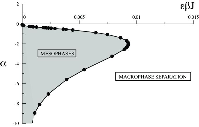
Figure 2: Theoretical phase diagram of the bi-lipidic fluctuating membrane in the plane ($\epsilon\beta J$, $\alpha$) at the onset of the macro-phase separation, i.e. at the critical temperature $T_{c}$. The gray region corresponds to the parameter range for which a phase separation occurs at a non-zero wave vector ${\tilde{q}}^{*}$ leading to the formation of mesophases instead of a macrophase separation.

On the experimental side, the parameters $\alpha$ and $\epsilon\beta J$ are not easy to determine. The phenomenological parameter $J$ coming from the Landau-Ginzburg theory, is somehow related to the van der Waals attractions between lipids and varies roughly as $1/T$ such that $\beta J$ is fixed for given lipid types and independent on temperature. Although we do not know exactly the value of this parameter, we can assume $\beta J\sim 1$. For lipidic vesicles made of a mixing of two very different lipids such as DMPC/cholesterol (a long lipid and a short one), the curvature modulus has been experimentally measured $\kappa_{0}\simeq 50\,k_{B}T$ ($26\,k_{B}T$ with DMPC alone) and increases when the proportion of cholesterol increases up to $250\,k_{B}T$ with 50% of cholesterol meleard ; duwe . Hence we find $\epsilon\beta J\sim 0.01$ which means that the mesophases region of the phase diagram can be experimentally reached in such systems.

Finally, in the mesophase region, the denominator of $S(q)$ given by Eq. (36) becomes negative and the calculation of the preceding sections, based on quadratic fluctuations of $\psi$ is no longer valid (the modes $q\approx q^{*}$ are unstable). The nature of the resulting stable mesophase requires further analysis to determine it and this is beyond the scope of the present paper.

VI Discussion and conclusions

In this paper we have shown that the coupling of membrane composition via a composition dependence on the local surface energy and bending rigidity can alter the phase diagram of a membrane composed of a mixture of different lipids. Indeed, depending on the physico-chemical properties of the lipids (for instance by modifying the length of their hydrophobic tail), the membrane can exhibits a micro-phase separation leading to the formation of so-called mesophases at a temperature $T>T_{c}$, i.e. before an eventual macro-phase separation. In the previous works where surface tension was considered the composition–fluctuation coupling was linear and the up-down symmetry of the system thus broken.

The long-range part of the interaction given by Eq. (26) behaves as $-1/r^{4}$ for large $r$. This interaction has the same behavior as that found between inclusions in several models where surface tension is not present. For instance in tensionless membranes one finds the effective pairwise interaction gou1 ; palu

$$V_{C}(r)=-k_{B}T\,6\pi^{2}\left(\frac{r_{0}}{r}\right)^{4}$$ (42)

between circular inclusions with the up-down symmetry, where $r_{0}$ is the radius of the inclusions. The long-range part of the interaction found in Eq. (26)–(30) is also proportional to the thermal energy but it is solely due to fluctuations in the surface or elastic energy.

A few works focused on the effect of the surface tension on fluctuation induced interactions sens ; sens2 ; sepangi ; misbah2 . Calculating the potential between two circular inclusions which locally apply a pressure on the membrane, Evans et al. found an interaction which is everywhere repulsive sens between inclusions of the same type and is given by

$$\Phi(r)=\frac{\zeta_{1}\zeta_{2}}{2\pi\gamma}K_{0}(mr),$$ (43)

where $\zeta_{i}$ is related to the force distribution of inclusions $i$ acting on the membrane surface and $\gamma$ is the surface tension. Here again, this interaction is different from Eq. (26) in origin but has some similar features: it is present for membranes under tension and is repulsive with a typical range of $\xi\simeq 30$ nm for biological membranes. Our model is very different, it does not assume any pressure distribution acting on the membrane but relies on the behavior of $\kappa(\phi)$ and $V(\phi)$ close to a liquid-liquid immiscibility critical point. This proximity to a liquid-liquid immiscibility critical point in a real biological context is supported by beautiful experiments on mono-layers made of lipids extracted from erythrocytes keller .

In this study we have seen that the induced interaction only has a repulsive when component when $\alpha<0$. Qualitatively, this means that the signs of $\kappa^{\prime}(\phi_{0})$ and $V^{\prime}(\phi_{0})$ are opposite: when a region is locally enriched for instance in lipid $A$, bending rigidity increased ($\kappa^{\prime}(\phi_{0})>0$) whereas the effective surface tension decreases ($V^{\prime}(\phi_{0})<0$). Let us consider for a moment the mean-field theory where one neglects the fluctuations $\psi$ about $\phi_{0}$. Consider an incompressible membrane which is constrained to have a constant projected area, for example a membrane supported by a frame. Also let the membrane exchange lipid species with the bulk solution around it fapi . The mean-field free energy as a function of $\phi_{0}$ is given from Eq. (14) as

$${F(\phi_{0})\over A}=V(\phi_{0})+{1\over 4\pi\beta}\int_{0}^{\Lambda}kdk\ln\left[\kappa(\phi_{0})k^{4}+V(\phi_{0})k^{2}\right]$$ (44)

This mean-field free energy must be regularized by the ultra-violet cut-off $\Lambda$. As the membrane is in a solution containing a reservoir of lipid species, $\phi_{0}$ is not fixed but is thermodynamically selected so as to minimize the mean-field free energy. In this case, in our previous treatment we should have thus included a term $V^{\prime}(\phi_{0})\psi$ in the expression for $H_{0}^{I}$, however this term can be seen to cancel exactly with the first term of the cumulant expansion, which in this case is also now no longer zero. The part of the free energy $F^{*}$ which varies with $\phi_{0}$ is given by

$${F^{*}(\phi_{0})\over A}=V(\phi_{0})+{1\over 8\pi\beta}\left[\Lambda^{2}\ln\left(\kappa(\phi_{0})+{V(\phi_{0})\over\Lambda^{2}}\right)+{V(\phi_{0})\over\kappa(\phi_{0})}\ln\left({\kappa(\phi_{0})\Lambda^{2}\over V(\phi_{0})}+1\right)\right].$$ (45)

The calculation carried out in this paper is valid for small surface fluctuations, a way of ensuring that the fluctuations are small is by choosing a very stiff membrane. This can be ensured by taking $\kappa(\phi)$ large. The equation minimizing $F^{*}(\phi_{0})$ can be expressed as

$$V^{\prime}(\phi_{0})\left[1+{1\over 4\pi\beta}\int_{0}^{\Lambda}kdk\ {1\over\kappa(\phi_{0})k^{2}+V(\phi_{0})}\right]+{\kappa^{\prime}(\phi_{0})\over 4\pi\beta}\int_{0}^{\Lambda}kdk\ {k^{2}\over\kappa(\phi_{0})k^{2}+V(\phi_{0})}=0.$$ (46)

Now physically we must have $V(\phi_{0})>0$, as for any effective surface tension (it is necessary to have $m$ real), this result implies that the system will naturally be in the region where $\alpha<0$. Now it is straightforward to show, see for example safran , at the the mean field level used here that ratio of the excess area to the projected area is given as

$${\Delta A\over A}={1\over 4\pi\beta}\int_{0}^{\Lambda}kdk\ {1\over\kappa(\phi_{0})k^{2}+V(\phi_{0})}={1\over 8\pi\beta\kappa(\phi_{0})}\ln\left({\kappa(\phi_{0})\Lambda^{2}\over V(\phi_{0})}+1\right).$$ (47)

In terms of the ratio of the excess to projected area, equation 46 can now be written as

$$V^{\prime}(\phi_{0})\left[1+{\Delta A\over A}\right]+{\kappa^{\prime}(\phi_{0})\over\kappa(\phi_{0})}\left[{\Lambda^{2}\over 8\pi\beta}-{V(\phi_{0})\Delta A\over A}\right]=0$$ (48)

In the limit where $\Delta A/A$ is small using Eq. (28) we obtain

$$\alpha=-{\Lambda^{2}\over 8\pi\beta V(\phi_{0})},$$ (49)

Now if we write $\Lambda=2\pi/a$ where $a$ is the microscopic length scale we find that

$$\alpha=-{\pi k_{B}T\over 2\epsilon_{a}}$$ (50)

where $\epsilon_{a}$ is the surface energy of a square of the membrane of linear dimension $a$, i.e. the average surface energy per lipid. Hence we find $\alpha<0$ which suggests a scenario to observe the formation of mesophases experimentally. For instance one can use a membrane composed by a mixture of DPMC/cholesterol and supported by a frame close at a temperature close to $T_{c}$.

In a more general context, molecular dynamics imparato and Monte Carlo simulations brown have shown that the bending rigidity has a non-monotonic behavior as a function of the short lipid number fraction $x_{s}$: it first decreases rapidly for small $x_{s}$ and then increases slowly, with a minimum around $x_{s}\simeq 0.6$. These studies suggest that for a two-component bilayer made of short and long lipids, the gradient of $\kappa(\phi)$ and $V(\phi)$ could have opposite signs but some tuning may be required. In this case the effective interaction will have a repulsive component which could induce mesoscopic phase separation.

The issue of mesophase formation has been discussed in several papers. Taniguchi tani has shown in a model with a linear coupling of the composition $\phi$ to the mean curvature that near to spherical vesicles with off-critical compositions exhibit circular domains that closely resemble patterns observed in red blood cell echinocytosis keller .

A similar study has been carried out in different geometries saxena and the same general phenomena are observed. Inspired by the problem of pattern formation of quantum dots at the air-water interface, Sear et al. sear have studied the effects of a short-range attraction (on top of a shorter range hard core) and long-range repulsion in Monte Carlo simulations of two dimensional systems of interacting particles. In their simulations both circular domains and stripes were observed as is the case in the experiments.

Finally, by adding an attractive short-range interaction to the potential Eq. (43), Evans et al. have argued that mesophase formation sens could be induced. Hence, it could explain the formation of caveolae buds from cell membranes and their striped texture. The mechanism proposed in this paper of course leads to the same phenomenology in the case where the effective potential induced by membrane fluctuations has an intermediate range repulsive component. However we do not find any repulsion in the situation where $\alpha>0$ which implies some conditions on the membrane composition which could perhaps be tested experimentally.

The model presented in this paper can be generalized by considering lipid distributions without the up-down symmetry, i.e. with different compositions in the up and bottom leaves. In this case, one would introduce a composition dependent spontaneous curvature, $c(\phi)$ in the Hamiltonian. If one assumes that the mixed homogeneous phase has no spontaneous curvature then one takes $c(\phi_{0})=0$ and in this case the correction to the long-range interaction is

$$v^{*}(r)=-\frac{V(\phi_{0})}{2\pi}[c^{\prime}(\phi_{0})]^{2}K_{0}(mr)$$ (51)

and the mass is renormalized (by a repulsive term). Hence this correction is attractive and could wipe out the above repulsive effect. The two-component membrane could also contain trans-membrane proteins. Despite the fact that the repulsive interaction between inclusions described by Evans et al. would appear, it is well known that protein aggregation also increases the local lipid composition, as observed in erythrocyte membranes where it induces a phospholipid enrichment rodgers . The inclusion of protein-like insertions in this two-lipid model could thus produce quite rich behavior and is a line worth pursuing.

Our study has predicted that it is possible that a membrane whose fluctuations are impeded exhibits a macro-phase separation whereas if it is allowed to fluctuate freely this transition becomes a mesophase separation . In a stack of membranes the fluctuations are suppressed by Helfrich forces helf which are of steric origin. Experimentally, therefore, one could prepare a stack of bilayers at a lipid composition where the bilayers within the stack exhibit a macro-phase separation. However, according to our predictions, a single membrane could possibly exhibit a mesophase separation lau . Another possibility is that one could try and observe the effect predicted here by using charged membranes and then varying their rigidity by changing the bulk solution’s salt content winh .

We emphasize that, in this paper, we have concentrated on an entirely equilibrium mechanism as a possible explanation for the formation of mesoscopic domains. However in living cells, out of equilibrium effects are of course important. Recently the recycling of lipids between the membrane and cell interior has been put forward as a non-equilibrium mechanism for the formation of raft-like structures in active systems foret ; tuse .

References

- (1) W. Helfrich, Z. Naturforsch. 28c, 693 (1973).
- (2) U. Seifert. Adv. Phys. 46 13, (1997).
- (3) B. Alberts et al. Molecular Biology of the Cell (Taylor and Francis Group, New York, 2002) 4th ed.
- (4) R. Lipowsky, J. Phys. II France 2 1825, (1992).
- (5) F. Jülicher and R. Lipowsky, Phys. Rev. E 53, 2670 (1996).
- (6) M. Goulian, R. Bruinsma, and P. Pincus, Europhys. Lett. 22, 145 (1993).
- (7) M. Goulian, Curr. Opin. Colloid Interface Sci. 1, 358 (1996).
- (8) K.S. Kim, J. Neu, and G. Oster, Biophys. J. 75, 2274 (1998).
- (9) J. M. Park, and T.C. Lubensky, J. Phys. I 6, 1217 (1996).
- (10) J.-B. Fournier and P.G. Dommersnes, Eur. Phys. J. B 12, 9 (1999).
- (11) J.-B. Fournier and P.G. Dommersnes, Biophys. J. 83, 2898 (2002).
- (12) V. I. Marchenko, and C. Misbah, Eur. Phys. J. E 8, 477 (2002).
- (13) D. Bartolo and J.-B. Fournier, Eur. Phys. J. E 11, 141 (2003).
- (14) R. Golestanian, M. Goulian, and M. Kardar, Phys. Rev. E, 54, 6725 (1996).
- (15) S. Leibler, J. Phys. (Paris) 47, 506 (1986).
- (16) T. Taniguchi, Phys. Rev. Lett. 76, 4444 (1996).
- (17) Y. Jiang, T. Lookman, and A. Saxena, Phys. Rev. E, 61, R57 (2000).
- (18) F. Divet, G. Danker, and C. Misbah, Phys. Rev. E, 72 041901 (2005).
- (19) R.R. Netz, J. Phys. I France 7, 833 (1997).
- (20) R.R. Netz and P. Pincus, Phys. Rev. E 52, 4114 (1995).
- (21) R. Bar-Ziv, T. Frisch and E. Moses, Phys. Rev. Lett. 75, 3481 (1995).
- (22) A.R. Evans, M.S. Turner, and P. Sens, Phys. Rev. E 67, 041907 (2003).
- (23) M.S. Turner and P. Sens, Biophys. J., 76, 564 (1999).
- (24) S.L. Keller, W.H. Pitcher III, W.H. Huestis, and H.M. McConnell, Phys. Rev. Lett. 81, 5019 (1998).
- (25) R.P. Sear, S.-W. Chung, G. Markovich, W.M. Gelbart, and J.R. Heath, Phys. Rev. E 59, R6255 (1999).
- (26) T.R. Weikl, M.M. Kozlov and W. Helfrich Phys. Rev. E 57, 6988 (1999).
- (27) M. Abramowitz and I.A. Stegun, Handbook of mathematical functions Dover, (1965).
- (28) P. Méleard et al., Biophys.J. 72, 2616 (1997).
- (29) H.P. Duwe, J. Käs, and E. Sackmann, J. Phys. france 51, 945 (1990).
- (30) H. Rafii-Tabar and H.R. Sepangi, arXiv:cond-mat/0508718.
- (31) S.A. Safran, Statistical Thermodynamics of Surfaces, Interfaces, and Membranes Westview, (2003).
- (32) O. Farago and P. Pincus, Eur. Phys. J. E 11, 399 (2003).
- (33) A. Imparato, J.C. Shillcock, and R. Lipowsky, Europhys. Lett. 69, 650 (2005).
- (34) G. Brannigan and F.L.H. Brown, J. Chem. Phys. 122, 074905, (2005).
- (35) W. Rodgers and M. Glaser, PNAS 88, 1364 (1991).
- (36) W. Helfrich, Z. Naturforsch. 33ac, 305 (1978).
- (37) L. Salomé Private Communication
- (38) M. Winterhalter and W. Helfrich, J. Phys. Chem. 92, 6865 (1988).
- (39) L. Foret, Europhys. Lett. 71, 508 (2005).
- (40) M.S. Turner, P. Sens, and N.D. Socci, Phys. Rev. Lett. 95, 168301 (2005).