Lecture Notes: Fundamental Problems in Statistical Mechanics XI,
Leuven, September 4 - 16, 2005





Exact solutions for KPZ-type growth processes,
random matrices,
and equilibrium shapes of crystals

Abstract: Three models from statistical physics can be analyzed by employing space-time determinantal processes: (1) crystal facets, in particular the statistical properties of the facet edge, and equivalently tilings of the plane, (2) one-dimensional growth processes in the Kardar-Parisi-Zhang universality class and directed last passage percolation, (3) random matrices, multi-matrix models, and Dyson’s Brownian motion. We explain the method and survey results of physical interest.

1 Introduction

Exactly solvable models from Equilibrium Statistical Mechanics in two space-dimensions are a continuing source of fascinating research. Historically the Onsager solution of the two-dimensional Ising model stands out. But the field has progressed. The most recent advance is conformal field theory and its probabilistic underpinning through the link to the Schramm-Loewner evolution (SLE) [8].

Going back to the Ph.D. thesis of Ising, one conventional starting point for an exact solution in equilibrium statistical mechanics is to write the Boltzmann weight as a product of matrices. Each factor is referred to as transfer matrix. In case of a spin system on the two-dimensional lattice $\mathbb{Z}^{2}$ the matrix elements of the transfer matrix are labeled by spin configurations in adjacent columns. Under favorable circumstances the transfer matrix can be rewritten as the configuration space kernel of $\exp[-H]$, where $H$ is bilinear in fermionic creation/annihilation operators labeled by the sites of a single column. In such case one says that the model can be solved through a mapping to free fermions. The problem of finding the largest eigenvalue of the $2^{N}\times 2^{N}$ transfer matrix is reduced to the eigenvalue problem of an $N\times N$ matrix. For the 2D Ising model the free fermion method was discovered by Lieb, Mattis and Schultz [41]. Under less favorable circumstances one can still extract information from the transfer matrix by more sophisticated methods, like the Bethe ansatz, the Yang-Baxter equations, and the technique of commuting transfer matrices. We refer to [32, 6] for details. For the purpose of our lectures the free fermion method with suitable extensions will do.

To be more concrete, and to anticipate some features to be developed in much greater depth further on, let us explain the free fermion method in the context of the ANNNI model [46], to say the 2D anisotropic next nearest neighbor Ising model. The spins, with values $\pm 1$, are located at the sites of the square lattice $\mathbb{Z}^{2}$. Because of anisotropy the properties in the 1- and 2-direction are very different. It is then convenient to consider the 1-axis as fictitious “time” and the 2-axis as “space”. Along the time direction the spins interact via the ferromagnetic nearest neighbor coupling $J_{0}$, $J_{0}>0$, while in the space direction there is a nearest neighbor ferromagnetic coupling $J_{1}$ and a next nearest neighbor antiferromagnetic coupling $J_{2}$. We set $J_{2}=-J_{1}/2<0$. The ground state is then highly degenerate. It consists of alternating strips of $+$ spins and $-$ spins parallel to the time direction with a width of 2 or larger.

As the temperature is increased, the domain walls, i.e., the lines separating the $+$ and $-$ domains, become thermally rough. In approximation we postulate that a domain wall has up-steps and down-steps of size 1 only and has no overhangs, see Figure 1(a). To have easier comparison with the models to be discussed below, the distance between neighboring domain walls is diminished by one lattice spacing. Then we obtain the following line ensemble: There are $M$ domain walls $t\mapsto x_{j}(t)$, $j=1,\ldots,M$, with $x_{j}\in[-N,\ldots,N]$, $t\in[-N,\ldots,N]$. Each domain wall has steps at most of size 1, $x_{j}(t+1)-x_{j}(t)=0,\pm 1$ for all $j,t$, and the domain walls satisfy the non-crossing (non-intersecting) constraint $x_{j}(t)<x_{j+1}(t)$. To an admissible configuration of domain walls one assigns a Boltzmann weight. A single step of the domain wall has weight $e^{-J_{0}/k_{\mathrm{B}}T}$. Thus the Boltzmann weight for a configuration of admissible domain walls is

$$\exp{\big{[}}-\tfrac{J_{0}}{k_{\mathrm{B}}T}{\textrm{(number of up-steps and down-steps)}}{\big{]}}\,.$$

So far we have imposed a hard wall boundary condition in the space and free boundary conditions in the time direction. One could also require periodic boundary conditions in the $t$-direction. A further popular choice are in addition chiral boundary conditions along the space direction. Then the domain walls have a nonzero slope on average.

The low temperature phase diagram of the ANNNI model, in the approximation just explained, can by analyzed using free fermions. Since we will have ample opportunity to explain the method, no details are needed now. Let me emphasize that, while anisotropic, the ANNNI model as defined is translation invariant. Thus the interest is in the free energy per unit volume and in the two-point function which depends only on the relative distance of the two points. In contrast, the topic of my lectures is concerned with line ensembles which are inhomogeneous both in space and time. Figure 1 illustrates the difference.

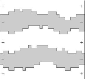
Figure 1: (a) Domain walls of the ANNNI model and (b) line ensemble of the PNG growth model. Note that for the line ensemble (b) there is a top line. Mostly, our focus will be on the statistical properties of the top line.

Over the past six years, for some instants even much further back, it has been recognized that there are three physically very distinct systems which can be analyzed through inhomogeneous line ensembles, namely

• crystal facets, in particular the statistical properties of the facet edge, and equivalently tilings of the plane,

• one-dimensional growth processes in the Kardar-Parisi-Zhang universality class and directed last passage percolation,

• random matrices, multi-matrix models, and Dyson’s Brownian motion.

In the first item the description through a line ensemble is rather immediate, as it is in the last item when focusing on Dyson’s Brownian motion. For growth processes the link turns out to be more hidden.

Our plan is to explain, in fair detail, for the three items listed how the physical model is mapped to a line ensemble with determinantal correlations. I want to provide the reader with a feeling for the method, in particular its flexibility and its limitations. Thereby one has not yet gained any understanding of the statistical properties of the model, but one has reached the “trail head” for a hike towards the summit by means of rather formidable asymptotic analysis. The details of the hike are well documented in the literature and I will make no attempt to duplicate. However, I will discuss of what one learns about crystal facets and growth models beyond the specific “exactly solved” model.

The main technical tool will be determinantal point processes, which are discussed per se in the following section. The application to statistical mechanics models will occupy the remainder of the survey.
Acknowledgements. My article is based on the Ph.D. thesis of Michael Prähofer [35] and on the Ph.D. thesis of Patrik Ferrari [11]. I am very grateful for their sharing of insights and the ongoing collaboration. In addition, I thank Patrik Ferrari for supplying the figures.

2 Determinantal point processes

The correlation functions of a determinantal point process are computable from a single correlation (two-point) kernel. In this respect, although otherwise very different, determinantal point processes are similar to Gaussian random fields. Therefore we first recall briefly
Gaussian processes. In the discrete setting one starts from the family of mean zero Gaussian random variables $X_{1},\ldots,X_{N}$. Their covariance matrix is

$$C(i,j)=\langle X_{i}X_{j}\rangle\,.$$ (2.1)

Clearly $C(i,j)=C(j,i)$ and $C\geq 0$ as a matrix. Conversely, every such matrix is the covariance of a Gaussian process. Higher moments are computable through the pairing rule

$$\langle\prod^{2m}_{\ell=1}X_{j_{\ell}}\rangle=\sum_{{\mathrm{pairings}}\,\pi(k),\pi^{\prime}(k)}\prod^{m}_{k=1}C\big{(}\pi(k),\pi^{\prime}(k)\big{)}\,,$$ (2.2)

where the sum is over all possible pairings of the indices $j_{1},\ldots,j_{2m}$. An index is allowed to appear several times in the list.

Since also space-time processes will be in demand, we add the time index $t\in[0,T]$. We have then the family of mean zero Gaussian processes $X_{1}(t),\ldots,X_{N}(t)$. As before their covariance matrix is

$$C(i,s;j,t)=\langle X_{i}(s)X_{j}(t)\rangle$$ (2.3)

considered as a positive operator on $\mathbb{C}^{N}\otimes L^{2}([0,T])$. Except for being continuous, the time-index $t$ is on the same footing as the space-index $j$. In particular, the pairing rule (2.2) is still valid.

With this background let us discuss determinantal point processes which is done in two steps, static and dynamic.
Determinantal point processes, spatial part. For simplicity let us first assume space to be discrete. At each site $j\in[1,\ldots,N]$ there is an occupation variable $\eta_{j}=0,1$, where 0 stands for empty and 1 for occupied, which is the reason for the name “point process”. We prescribe a hermitian matrix $R(i,j)$ such that $0\leq R\leq 1$. Then the joint distribution of the $\eta$’s is defined through the moments

$$\langle\prod^{m}_{k=1}\eta_{j_{k}}\rangle=\det\big{(}R(j_{\ell},j_{\ell^{\prime}})\big{)}_{1\leq\ell,\ell^{\prime}\leq m}\,,$$ (2.4)

provided the collection of indices $\{j_{1},\ldots,j_{m}\}$ has no double points. As for Gaussians there is the single correlation kernel $R$ which fixes the full probability distribution. However, note that two different $R$ kernels may give rise to the same $\eta$-distribution. In the applications below, we will meet a real $R$ matrix which is self-similar to a symmetric matrix $\widetilde{R}$, i.e., $R(i,j)=g(i)\widetilde{R}(i,j)g(j)^{-1}$. Clearly, according to (2.4), the moments do not depend on whether they are computed from $R$ or $\widetilde{R}$.

To understand the connection to free fermions let us introduce the fermion algebra $a_{j}$, $j=1,\ldots,N$, satisfying the anticommutation relations

$$\{a_{i},a_{j}\}=0\,,\;\{a_{i}^{\ast},a_{j}^{\ast}\}=0\,,\;\{a_{i},a_{j}^{\ast}\}=\delta_{ij}$$ (2.5)

with the anticommutator $\{A,B\}=AB+BA$. Let

$$H=\sum^{N}_{i,j=1}a^{\ast}_{i}\mathfrak{h}_{ij}a_{j}$$ (2.6)

be a quadratic fermion operator with $\mathfrak{h}$ the $N\times N$ one-particle Hamiltonian. $H=H^{\ast}$ is equivalent to $\mathfrak{h}$ being hermitian, $\mathfrak{h}=\mathfrak{h}^{\ast}$. We then set $\eta_{j}=a^{\ast}_{j}a_{j}$, the fermionic occupation variables, and

$$\langle\prod^{m}_{k=1}\eta_{j_{k}}\rangle=Z^{-1}\mathrm{tr}\big{[}e^{-H}\prod^{m}_{k=1}a^{\ast}_{j_{k}}a_{j_{k}}\big{]}\,,\quad Z=\mathrm{tr}\big{[}e^{-H}\big{]}\,.$$ (2.7)

It is an exercise in anticommutators to verify that the moments of the occupation variables are determinantal with correlation kernel

$$R(i,j)=Z^{-1}\mathrm{tr}\big{[}e^{-H}a^{\ast}_{i}a_{j}\big{]}=\big{(}(1+e^{\mathfrak{h}})^{-1}\big{)}_{ji}\,.$$ (2.8)

Later on a prominent quantity will be the probability for the set $B\subset[1,\ldots,N]$ to be empty. To compute it one could use (2.4); however the fermions offer a shortcut. Let $\chi_{B}$ be the indicator function for the set $B$ and let $N_{B}=\sum_{j\in B}a^{\ast}_{j}a_{j}$. Then, with $\mathbb{P}(\cdot)$ our generic symbol for probability,

$$\mathbb{P}(\eta_{j}=0,j\in B)=\lim_{\lambda\to\infty}Z^{-1}\mathrm{tr}\big{[}e^{-H}e^{-\lambda N_{B}}\big{]}$$

$$\hskip 36.0pt=\lim_{\lambda\to\infty}(\det(1+e^{\mathfrak{-h}}))^{-1}\det(1+e^{\mathfrak{-h}}e^{-\lambda\chi_{B}})$$

$$\hskip 36.0pt=\det(1-\chi_{B}R\chi_{B})\,.$$ (2.9)

To define determinantal processes over a continuum rather than discrete space is as simple as for Gaussian processes [42]. Let $\eta(x)$, $0\leq x\leq\ell$, be the point process. Every realization is of the form

$$\eta(x)=\sum^{n}_{j=1}\delta(x-y_{j})\,,\quad y_{j}\in[0,\ell]\,.$$ (2.10)

Here $n$ is arbitrary and $n=0$ means no point in $[0,\ell]$. Furthermore we prescribe the correlation kernel through a linear operator $R$ on $L^{2}([0,\ell])$ with $R=R^{\ast}$, $0\leq R\leq 1$, and $\mathrm{tr}R<\infty$. Then, provided $\{x_{1},\ldots,x_{m}\}$ has no double points, one defines

$$\langle\prod^{m}_{k=1}\eta(x_{k})\rangle=\det\big{(}R(x_{\ell},x_{\ell^{\prime}})\big{)}_{1\leq\ell,\ell^{\prime}\leq m}\,.\vskip 3.0pt plus 1.0pt minus 1.0pt$$ (2.11)

Extended determinantal point processes. To extend determinantal processes to space-time, it is tempting to follow the Gaussian example by introducing a space index $j$ and a time index $t\in[0,T]$. Then, according to the definitions above, $\eta_{j}(t)$ would be concentrated on a collection of points in $[1,\ldots,N]\times[0,T]$, which is not a line ensemble of the form anticipated in the Introduction. Thus, to properly guess the correct structure, we turn to the example of $n$ non-intersecting Brownian paths pinned at both ends to the origin, which goes back to Karlin and McGregor [27]. With such a constraint and boundary condition typical paths resemble vaguely a watermelon, compare with Figure 2.

\psfrag{0}[r]{$0$}\psfrag{T}[l]{$T$}\psfrag{t}{$t$}\psfrag{x}{$x$}\includegraphics[height=142.26378pt]{Watermelon.eps}

Figure 2: Pinned Brownian motion conditioned not to intersect, also referred to as watermelon ensemble.

More precisely, for $j=1,\ldots,n$, $t\mapsto x_{j}(t)$, $0\leq t\leq T$, is a one-dimensional Brownian motion pinned such that $x_{j}(0)=0$, $x_{j}(T)=0$. In addition we impose the constraint of non-crossing as

$$x_{j}(t)<x_{j+1}(t)\,,\quad 0<t<T\,,\quad j=1,\ldots,n-1\,.$$ (2.12)

The corresponding random field over $\mathbb{R}\times[0,T]$ is then

$$\eta(x,t)=\sum^{n}_{j=1}\delta\big{(}x-x_{j}(t)\big{)}\,.$$ (2.13)

If $T$ and $n$ are of the same order, then the constraint pushes the top line a distance $T$ away from the origin, which is to be compared with the typical $\sqrt{T}$ fluctuations for a single Brownian bridge. Since the repulsion originates in a mere constraint in the number of configurations, it is known as entropic repulsion.

Let us first consider a single line, $n=1$. If the Gaussian transition probability, from $x$ to $y$ in time $t$, is denoted by

$$p_{t}(x,y)=\frac{1}{\sqrt{2\pi t}}e^{-(y-x)^{2}/2t}\,,$$ (2.14)

one obtains

$$\mathbb{P}_{0,0}\big{(}x_{1}(t)\in[x,x+dx]\big{)}=p_{T}(0,0)^{-1}p_{t}(0,x)p_{T-t}(x,0)dx\,,$$ (2.15)

where the subscript 0,0 reminds of the pinning to zero at both ends. $p_{T}(0,0)^{-1}$ is the proper normalization.

Next let us consider two lines, but for simplicity only the point statistics at fixed $t$. By the reflection principle, for arbitrary starting points $x_{j}(0)=x_{j}$, $j=1,2$, $x_{1}<x_{2}$, and unconstrained end points, one has the conditional probability

$$\mathbb{P}\big{(}x_{1}(t)\in[y_{1},y_{1}+dy_{1}],x_{2}(t)\in[y_{2},y_{2}+dy_{2}]\,|\,x_{1}(0)=x_{1},x_{2}(0)=x_{2},$$

$$\hskip 180.0ptx_{1}(s)<x_{2}(s)\;\mathrm{for}\;0\leq s\leq t\big{)}$$

$$=Z(t,x_{1},x_{2})^{-1}\big{(}p_{t}(x_{1},y_{1})p_{t}(x_{2},y_{2})-p_{t}(x_{1},y_{2})p_{t}(x_{2},y_{1})\big{)}\theta(y_{2}-y_{1})dy_{1}dy_{2}$$

with $\theta(u)=1$ for $u\geq 0$, $\theta(u)=0$ for $u<0$, and $Z$ the normalization. Therefore, with pinning at 0 and normalizing partition function $Z(\delta)$,

$$\mathbb{P}_{0,0}\big{(}x_{1}(t)\in[x_{1},x_{1}+dx_{1}],x_{2}(t)\in[x_{2},x_{2}+dx_{2}]\big{)}$$

$$=\lim_{\delta\to 0}Z(\delta)^{-1}\big{[}p_{t}(0,x_{1})p_{t}(\delta,x_{2})-p_{t}(0,x_{2})p_{t}(\delta,x_{1})\big{]}$$

$$\hskip 36.0pt\times\big{[}p_{T-t}(x_{1},0)p_{T-t}(x_{2},\delta)-p_{T-t}(x_{2},0)p_{T-t}(x_{1},\delta)\big{]}dx_{1}dx_{2}$$

$$=\big{(}R(x_{1},x_{1})R(x_{2},x_{2})-R(x_{1},x_{2})R(x_{2},x_{1})\big{)}dx_{1}dx_{2}\,,$$ (2.17)

where

$$R(x,y)=p_{t}(0,x)p_{T-t}(y,0)\big{(}p_{T}(0,0)^{-1}+Z^{-1}_{2}xy\big{)}\,,$$

$$Z_{2}=\int p_{t}(0,x)x^{2}p_{T-t}(x,0)dx\,.$$ (2.18)

Clearly, for fixed $t$ and $n=2$, the point process $\eta(x,t)$ of (2.13) is determinantal.

To extend to general $n$, still at fixed time $t$, it is convenient to first introduce the Fermi field over $\mathbb{R}$ with creation/annihilation operators satisfying the anticommutation relations

$$\{a(x),a(x^{\prime})\}=0\,,\;\{a^{\ast}(x),a^{\ast}(x^{\prime})\}=0\,,\;\{a(x),a^{\ast}(x^{\prime})\}=\delta(x-x^{\prime})\,,\;x,x^{\prime}\in\mathbb{R}\,.$$ (2.19)

To have a concise notation one also introduces the harmonic oscillator Hamiltonian with frequency $1/t$ as

$$\mathfrak{h}_{t}=\frac{1}{2}\big{(}\!-\frac{d^{2}}{dx^{2}}+\frac{1}{t^{2}}x^{2}\big{)}\,,$$ (2.20)

and its second quantization

$$H_{t}=\frac{1}{2}\int a^{\ast}(x)\big{(}\!-\frac{d^{2}}{dx^{2}}+\frac{1}{t^{2}}x^{2}\big{)}a(x)dx\,.$$ (2.21)

We now proceed as in (2), but for $n$ lines. In the limit $\delta\to 0$ the left factor becomes $\psi^{(n)}_{t}$ and the right factor $\psi^{(n)}_{T-t}$, where $\psi^{(n)}_{t}$ is the ground state for $H_{t}$ with $n$ fermions. Therefore

$$\langle\prod^{m}_{k=1}\eta(x_{k},t)\rangle=Z_{T}^{-1}\langle\psi^{(n)}_{T-t}|\prod^{m}_{k=1}a^{\ast}(x_{k})a(x_{k})|\psi^{(n)}_{t}\rangle_{\mathcal{F}}$$ (2.22)

with $Z_{T}=\langle\psi^{(n)}_{T-t}|\psi^{(n)}_{t}\rangle_{\mathcal{F}}$ and $\langle\cdot|\cdot\rangle_{\mathcal{F}}$ the inner product in fermionic Fock space. It is an exercise in anticommutators to confirm that the right hand side of (2.22) is determinantal with correlation kernel

$$R_{t}(x,x^{\prime})=Z_{T}^{-1}\langle\psi^{(n)}_{T-t}|a^{\ast}(x)a(x^{\prime})|\psi^{(n)}_{t}\rangle_{\mathcal{F}}\,.$$ (2.23)

One can use the normalized eigenfunctions $\varphi^{t}_{j}$ of $\mathfrak{h}_{t}$, i.e., the Hermite functions, to express $R_{t}$ as

$$R_{t}(x,x^{\prime})=\sum^{n-1}_{j=0}\varphi^{\tilde{t}}_{j}(x)\varphi^{\tilde{t}}_{j}(x^{\prime})$$ (2.24)

with $\tilde{t}=t(T-t)/T$. The correlation kernel is the Hermite kernel of order $n$.

With these preparations, we are in a position to attempt our goal, namely to extend to the point statistics at several times, e.g., to the joint probability distribution of $\eta(y_{1},t_{1})$ and $\eta(y_{2},t_{2})$, $0<t_{1}<t_{2}<T$. Of course, following the examples above, one can work out concrete formulas. They tend to be lengthy and it is more transparent to emphasize the general principle. The $n$-dependence turns out to be simple and we keep $n$ arbitrary, but the reader is invited to verify for $n=2$. From the limit $\delta\to 0$ at $t=0$ one obtains the ground state $\psi^{(n)}_{t_{1}}$ at time $t_{1}$, and correspondingly from the limit $\delta\to 0$ at $T$ one obtains $\psi^{(n)}_{T-t_{2}}$ at time $T-t_{2}$. For the propagation from $t_{1}$ to $t_{2}$, $\tau=t_{2}-t_{1}$, one has to use (2) for general $n$, which can be written as the position space kernel of $e^{-\tau G}$ restricted to the $n$-particle subspace, where

$$G=-\frac{1}{2}\int a^{\ast}(x)\frac{d^{2}}{dx^{2}}a(x)dx\,.$$ (2.25)

More explicitly, in position space,

$$\langle x_{1},\ldots,x_{n}\,|\,e^{-\tau G}\,|\,y_{1},\ldots,y_{n}\rangle=\det\big{(}p_{\tau}(x_{j}-y_{j^{\prime}})\big{)}_{1\leq j,j^{\prime}\leq n}\,.$$ (2.26)

Note that the free particle Hamiltonian $G$ provides the internal propagation, while the harmonic oscillator Hamiltonian $H_{t}$ reflects the pinning. Therefore

$$\langle\eta(y_{1},t_{1})\eta(y_{2},t_{2})\rangle=Z_{T}^{-1}\langle\psi^{(n)}_{T-t_{2}}|a^{\ast}(y_{2})a(y_{2})e^{-\tau G}a^{\ast}(y_{1})a(y_{1})|\psi^{(n)}_{t_{1}}\rangle_{\mathcal{F}}\$$ (2.27)

with $Z_{T}=\langle\psi^{(n)}_{T-t_{2}}|\psi^{(n)}_{t_{2}}\rangle_{\mathcal{F}}$.

It is yet another exercise in anticommutators to verify that the expression (2.27) is determinantal with the correlation kernel

$$R(x,t;x^{\prime},t^{\prime})=\begin{cases}Z_{T}^{-1}\langle\psi^{(n)}_{T-t}|a^{\ast}(x)e^{-|t-t^{\prime}|G}a(x^{\prime})|\psi^{(n)}_{t^{\prime}}\rangle_{\mathcal{F}}&\text{for}\;t\geq t^{\prime}\,,\\ -Z_{T}^{-1}\langle\psi^{(n)}_{T-t^{\prime}}|a(x^{\prime})e^{-|t-t^{\prime}|G}a^{\ast}(x)|\psi^{(n)}_{t}\rangle_{\mathcal{F}}&\text{for}\;t<t^{\prime}\,.\end{cases}$$ (2.28)

(2.27) generalizes to $m$ pairwise disjoint space-time points $(y_{1},t_{1}),\ldots,(y_{m},t_{m})$ which are ordered in time, i.e., $0<t_{1}\leq t_{2}\ldots\leq t_{m}<T$, as

$$\langle\prod^{m}_{j=1}\eta(y_{j},t_{j})\rangle=\det\big{(}R(y_{j},t_{j};y_{j^{\prime}},t_{j^{\prime}})\big{)}_{1\leq j,j^{\prime}\leq m}\,.$$ (2.29)

The moments are still of determinantal form. In contrast to the static rule, for space-time points the time order must be respected. On top the extended correlation kernel is not symmetric.

The general structure can be grasped even more clearly by returning to the discrete space setting from (2.5) above. In addition to the static Hamiltonian (2.6), there is the generator

$$G=\sum^{N}_{i,j=1}a^{\ast}_{i}\mathfrak{g}_{ij}a_{j}$$ (2.30)

for the time propagation. We define

$$a_{j}(t)=e^{tG}a_{j}e^{-tG}\,,\;a^{\ast}_{j}(t)=e^{tG}a^{\ast}_{j}e^{-tG}\,.$$ (2.31)

Then the dynamic extension of the static correlation kernel $R$ from (2.8) is given through

$$R(j,t;j^{\prime},t^{\prime})=\begin{cases}Z^{-1}\mathrm{tr}\big{[}e^{-H}e^{-TG}a^{\ast}_{j}(t)a_{j^{\prime}}(t^{\prime})\big{]}&\text{for}\;0\leq t^{\prime}\leq t\leq T\,,\\ -Z^{-1}\mathrm{tr}\big{[}e^{-H}e^{-TG}a_{j^{\prime}}(t^{\prime})a^{\ast}_{j}(t)\big{]}&\text{for}\;0\leq t<t^{\prime}\leq T\,,\end{cases}$$ (2.32)

where $Z=\mathrm{tr}\big{[}e^{-H}e^{-TG}\big{]}$.

In principle, the moments of the corresponding line ensemble are still defined via (2.29). For general $G$, one cannot expect that the so defined moments come from a probability measure. In fact, while $H$ can be arbitrary, except for $H=H^{\ast}$, the conditions on $G$ are rather stringent, as will be explained now, where we distinguish whether space, resp. time, is either continuous or discrete.
(1) continuous time, continuous space. In this case $\mathfrak{g}$ must be the generator of a diffusion process,

$$\mathfrak{g}(t)=-d(x,t)^{2}\frac{d^{2}}{dx^{2}}-a(x,t)\frac{d}{dx}+V(x,t)\,.$$ (2.33)

As for the watermelon, the line ensemble is constructed from independent lines with a weight determined by the propagator generated through $\mathfrak{g}(t)$ and subsequently imposing the nonintersecting constraint. The watermelon ensemble has constant diffusion and formally a strong confining potential at $t=0$ and $t=T$, $V(x,t)=0$ otherwise. As will be explained, the case $d=1$, $a=0$, $V(x)$ general corresponds to the eigenvalues of hermitian multi-matrix models.
(2) continuous time, discrete space. $\mathfrak{g}(t)$ is the generator of a continuous time nearest neighbor random walk. If space is $\mathbb{Z}$, then

$$(\mathfrak{g}(t)\psi)_{j}=-r_{+}(j,t)\psi_{j+1}-r_{-}(j,t)\psi_{j-1}+(r_{+}(j,t)+r_{-}(j,t)+V(j,t))\psi_{j}$$ (2.34)

with rates $r_{\pm}\geq 0$. For the polynuclear growth model we will encounter the simple random walk, for which $r_{+}(j)=r_{-}(j)=\frac{1}{2}$ and $V(j)=0$. As before, the line ensemble is obtained from independent lines by conditioning on non-crossing.

For discrete time, there seems to be no complete classification. Trivially, one can consider the cases (1) and (2) at discrete times $t=n\tau$ only. In addition one finds one-sided exponential, resp. geometric jumps.
(3) time discrete, space continuous. Let us take the ordered points $x_{1}<\ldots<x_{n}$. Then in an up-step the new configuration $\{x^{\prime}_{j},j=1,\ldots,n\}$ has to satisfy $x_{j}<x^{\prime}_{j}<x_{j+1}$, $j=1,\ldots,n$, formally $x_{n+1}=\infty$, and the weight is $\prod^{n}_{j=1}e^{-\delta(x^{\prime}_{j}-x_{j})}$, $\delta>0$. Our example may look artificial, but does turn up in the analysis of the totally asymmetric simple exclusion process.
(4) time discrete, space discrete. An obvious example are nearest neighbor discrete random walks. To have a meaningful non-crossing constraint odd and even sublattices must be properly adjusted, see Example (i) below. In case space is either $\mathbb{Z}$ or $\mathbb{Z}_{+}$, the analogue of one-sided exponential jumps are one-sided geometric jumps with weight $q^{n}$, where $n$ is the jump size, $n\geq 0$, and $0<q<1$. One-sided geometric jumps will show up for the Ising corner. In this model time $t\in\mathbb{Z}$, for $t<0$ one has only up-steps, and for $t\geq 0$ only down-steps, while the geometric parameter $q$ depends on $t$.

From the list above the guiding principle remains somewhat hidden. There is an alternative construction by Johansson [23, 25] which avoids fermions altogether and is based directly on a determinantal weight for the line ensemble. In the Addendum we outline a purely combinatorial scheme, which was devised by Gessel and Viennot as based on ideas of Lindström. All the examples from our list can be obtained through suitable limits of the Lindström-Gessel-Viennot scheme, which therefore can be regarded as the most general set-up for determinantal line ensembles.

Having the machinery of determinantal point processes at our disposal, we turn to models of statistical physics. They are crystals in thermal equilibrium (Section 3), growth processes (Sections 4, 5) and the eigenvalue statistics of random matrices (Section 6). Physical predictions are extracted from edge scaling. We also indicate briefly how through appropriate boundary conditions for the line ensemble further cases of physical interest can be handled.

Addendum: Nonintersecting paths on directed graphs without loops

We explain the Lindström-Gessel-Viennot theorem in the form stated by Stembridge [43]. One starts with a graph $(V,E)$ consisting of vertices $V$ and directed edges $E$. The graph has no loops. A path $P$ is a sequence of consecutive vertices joined by directed edges. $\mathcal{P}(u,v)$ denotes the set of all paths starting at $u\in V$ and ending at $v\in V$. The paths $P$ and $P^{\prime}$ intersect, if they have a common vertex. Every edge carries a weight $w(e)$ and every vertex a weight $\widetilde{w}(v)$. The weight of a path $P$ is hence given by

$$w(P)=\prod_{e\in P\cap E}w(e)\prod_{v\in P\cap V}\widetilde{w}(v)$$ (2.35)

and we set

$$h(u,v)=\sum_{P\in\mathcal{P}(u,v)}w(P)\,.$$ (2.36)

Let us now consider an $r$-tuple $\vec{u}=\{u_{1},\ldots,u_{r}\}$ of starting points and an $r$-tuple $\vec{v}=\{v_{1},\ldots,v_{r}\}$ of end points. Let $\mathcal{P}_{0}(\vec{u},\vec{v})$ be the set of all non-intersecting $r$-tuple of paths from $\vec{u}$ to $\vec{v}$. $\vec{u}$ and $\vec{v}$ have to be compatible, which means that any $r$-tuple of paths in $\mathcal{P}_{0}(\vec{u},\vec{v})$ necessarily connects $u_{j}$ to $v_{j}$ for $j=1,\ldots,r$. Then the weight of $\mathcal{P}_{0}(\vec{u},\vec{v})$ is given by

$$w(\mathcal{P}_{0}(\vec{u},\vec{v}))=\det\big{(}h(u_{i},v_{j})\big{)}_{1\leq i,j\leq r}\,.$$ (2.37)

\psfrag{w0}[lB]{$w_{0}$}\psfrag{wp}[c]{$w_{+}$}\psfrag{wm}[c]{$w_{-}$}\includegraphics[height=142.26378pt]{DPaztec.eps}

\psfrag{1}{$1$}\psfrag{q+}[c]{$q_{+}$}\psfrag{q-}[l]{$q_{-}$}\includegraphics[height=142.26378pt]{DPising.eps}

Figure 3: The directed graph for (a) the Aztec diamond and (b) the 3D Ising corner.

Let us illustrate the Gessel-Viennot scheme by a few examples.
(i) Simple random walks. Here $V=\mathbb{Z}^{2}$ restricted to the even sublattice and $E$ are all nearest neighbor edges, which are then directed either North-East or South-East. Their weight is $\widetilde{w}(v)=1$, $w(e)=w_{+}$ for $e$ directed NE, and $w(e)=w_{-}$ for $e$ directed SE.
(ii) Aztec diamond, domino tiling [22, 24], see Figure 3(a). Here $V=\mathbb{Z}^{2}$ and $E$ consists of all directed edges as in example (i) plus edges of the form $v$ directed to $v+(1,0)$. The horizontal edges have weight $w_{0}$, the NE edges weight $w_{+}$, and the SE edges weight $w_{-}$.
(iii) 3D Ising corner, lozenges tiling [15], see Figure 3(b). Here $V=(\mathbb{Z}\times\mathbb{Z})\cup((\mathbb{Z}+\frac{1}{2})\times\mathbb{Z})$. The horizontal edges are between nearest neighbors, directed East, and have weight 1. The vertical edges are nearest neighbor for $(\mathbb{Z}+\frac{1}{2})\times\mathbb{Z}$ only. If $\tau\in\mathbb{Z}+\frac{1}{2}$ is their 1-coordinate, then for $\tau<0$ they are directed North and for $\tau>0$ they are directed South with weight $q^{|\tau|}$, $0\leq q<1$.
(iv) Discrete time TASEP [21]. The setup is as in example (iii). Only the North and South directed edges are alternating with a $\tau$-independent weight $q\in[0,1)$. If the vertical lattice spacing is $\varepsilon$ and the weight is $q=1-\delta\varepsilon$, then in the limit $\varepsilon\to 0$ one obtains the one-sided exponential jumps from item (3) above.
(v) Six-vertex model at the free fermion point [12]. In the six-vertex model, see e.g. [32], one draws only the South and East pointing arrows. Because of the ice rule one then obtains a line ensemble. However lines may touch. To achieve non-intersecting lines, SE-edges are added but only for the even sublattice. Touching is avoided by choosing the SE short cut. There are then three weights, one for E-, SE-, and S-directed edges, respectively. Reconstructing the six-vertex weights one notices that they satisfy the free fermion condition. Rotating the space-time lattice by $\pi/4$ one arrives at Figure 3(a), only every second horizontal link is missing. They can be reintroduced, however, at the expense of splitting up the weight. Therefore the Aztec diamond is equivalent to the six-vertex model at its free fermion point.

3 Equilibrium crystal shape

As a rule crystals in thermal equilibrium are faceted at low temperatures. In this section we will discuss a simplified model, which can be analyzed through the method of determinantal line ensembles, see [15, 14].

We consider the simple cubic lattice $\mathbb{Z}^{3}$. Each site can be occupied by at most one atom and the occupation variables are denoted by $n_{x}=0,1$. If the nearest neighbor binding energy is $-J$, $J>0$, then the total binding energy of all atoms is given by

$$H=-\frac{J}{2}\sum_{|x-y|=1}n_{x}n_{y}\,.$$ (3.1)

At zero temperature only configurations of minimal energy are allowed. If exactly $N^{3}$ atoms are available, then they form a cube of side-length $N$. For concreteness we assume that the cube occupies the sites $[0,\ldots,N-1]^{3}\subset\mathbb{Z}^{3}$. If only $N^{3}-M$ atoms are available, with $M<N\ll N^{3}$, then the binding energy is reduced by $-3MJ$ compared to the perfect cube. However, now there are many configurations of minimal energy. They can be obtained by successively removing atoms from either one of the eight corners under the constraint to cut exactly three bonds in each step. Let us focus our attention at the corner touching the origin, compare with Figure 4.

\psfrag{1}[1]{$1$}\psfrag{2}[1]{$2$}\psfrag{3}[1]{$3$}\includegraphics[height=142.26378pt]{lozengeShaded.eps}

Figure 4: An atom configuration of the 3D Ising corner.

The atoms missing at that corner can then be enumerated ed by a height function $h(i,j)$, $i,j\geq 0$, taking only integer values such that

$$h(i,j)\geq 0\,,\;h(i,j)\geq h(i+1,j)\,,\;h(i,j)\geq h(i,j+1)\,,\;\lim_{i,j\to\infty}h(i,j)=0\,.$$ (3.2)

The atoms occupy the sites $\{x\,|\,x_{1}=i,x_{2}=j,x_{3}\geq h(i,j)\}$. E.g. the perfect cube corresponds to $h(i,j)=0$ for all $i,j$. The number (= volume) of removed atoms is

$$V(h)=\sum_{i,j\geq 0}h(i,j)\,.$$ (3.3)

In principle one should introduce such a height function for each corner and the volume constraint refers jointly to all corners. For simplicity we ignore such inessential complications, thus disregard the other corners, and impose the volume constraint on $h$ in the form

$$V(h)=M\,.$$ (3.4)

Every height configuration satisfying (3.2) and (3.4) has the same energy. Hence at zero temperature every configuration has the same weight and the model is purely entropic. The only task is to count.

To deal with the volume constraint it is convenient to switch to the grand canonical ensemble as

$$Z_{T}^{-1}e^{-V(h)/T}\,.$$ (3.5)

Here $T$ is the control parameter for the volume, not to be confused with the temperature. We are interested in a macroscopic volume, which corresponds to large $T$. Then the average volume, average with respect to (3.5), equals $\langle V\rangle_{T}\cong T^{3}$ and the height is typically of order $T$. Let us replace $h$ by $h_{T}$ in order to remember that the height statistics depends on $T$. We switch from $\mathbb{Z}^{3}$ to $(\mathbb{Z}/T)^{3}$, i.e., to a lattice spacing $1/T$ instead of 1. In the limit $T\to\infty$ fluctuations are suppressed and one observes a non-random macroscopic crystal shape, in formula

$$\lim_{T\to\infty}\frac{1}{T}h_{T}([uT],[vT])=h_{\mathrm{ma}}(u,v)$$ (3.6)

with probability one. Here $[\cdot]$ denotes the integer part, $u,v\geq 0$, and $h_{\mathrm{ma}}$ is the macroscopic crystal shape.

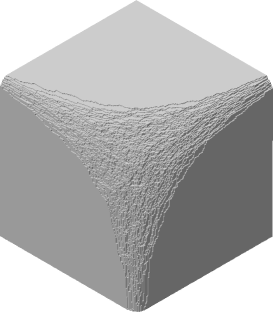
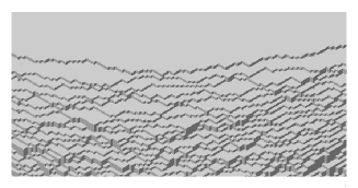
Figure 5: Monte-Carlo simulation of the 3D Ising corner with $M=3\times 10^{5}$ and an enlargement close to the facet edge.

In Figure 5 we display a typical atom configuration with volume constraint $M=3\times 10^{5}$. For the true crystal shape of the low temperature Ising model with volume constraint one has to imagine a perfect cube rounded at each corner as in Figure 5.

To have a nice looking formula for $h_{\mathrm{ma}}$, we choose the volume constraint as $2\zeta_{R}(3)T^{3}$ with $\zeta_{R}$ the Riemann zeta function. Let us define

$$f(a,b,c)=\frac{1}{4\pi^{2}}\int^{2\pi}_{0}du\int^{2\pi}_{0}dv\log(a+be^{iu}+ce^{iv})\,.$$ (3.7)

Then the set $S_{0}=\{(u,v,w)\,,\;u,v\geq 0\,,\;0\leq w\leq h_{\mathrm{ma}}(u,v)\}$ is parametrically given through

$$S_{0}=\{2(f(a,b,c)-\log a\,,\;f(a,b,c)-\log b\,,\;f(a,b,c)-\log c)\,|\;a,b,c>0\}\,.$$ (3.8)

As expected the equilibrium shape is symmetric relative to the (1,1,1) axis. Let $\mathcal{D}=\{(u,v)\,,\;e^{-u/2}+e^{-v/2}<1\}$. Then

$$h_{\mathrm{ma}}(u,v)=0\quad\mathrm{on}\;\mathbb{R}^{\,2}_{+}\setminus\mathcal{D}\,.$$ (3.9)

The equilibrium shape has three facets lying in the respective coordinate planes, see Figure 5. $\mathcal{D}$ is the domain where $h_{\mathrm{ma}}$ is rounded. Near the facet edge, in the direction $\tau=v-u$, one has

$$h_{\mathrm{ma}}(r,\tau)=\frac{2}{3}\cosh(\tau/4)\pi^{-1}2^{1/4}r^{3/2}\,,$$ (3.10)

valid for small $r$, where $r$ denotes the distance away from the edge. The 3/2-exponent is known as Pokrovsky-Talapov law [34].

The expression (3.7) has a simple physical meaning, for which we switch to the coordinate frame with (1,1,1) as 3-axis. As can be seen from Figure 4 the along (1,1,1) projected height profile yields a perfect tiling of the plane with lozenges which are oriented either with angle 0, or $2\pi/3$, or $4\pi/3$. Conversely, a tiling by lozenges such that asymptotically in each of the three segments there is only a single type translates back to an admissible height configuration. We now focus our attention on a small neighborhood of a point in $\mathcal{D}$. For large $T$ the curvature can be ignored and under projection the tiling is such that the fraction of each type of lozenges remains fixed. Again the grand canonical version is easier to control and we assign to the three types of lozenges the Boltzmann weights $a,b,c$, respectively. $f(a,b,c)$ from (3.7) is the free energy of such a tiling. Note that $f(\lambda a,\lambda b,\lambda c)=f(a,b,c)+\log\lambda$, as it has to be. A tiling of the plane corresponds to a flat surface with a non-random slope determined through $a,b,c$ and $f(a,b,c)$ takes the role of the surface tension.

Switching back to the original coordinate frame by this construction one obtains the surface tension $\sigma$ depending on the macroscopic slope $\nabla h$ of the height function. The explicit formula is unwieldy and not so instructive. We now give ourselves some macroscopic height profile $h$ defined on $(\mathbb{R}_{+})^{2}$. It must satisfy $h\geq 0$ and $\partial_{1}h\leq 0$, $\partial_{2}h\leq 0$. In the limit $T\to\infty$ the macroscopic free energy is additive and hence the prescribed profile $h$ has the total free energy

$$\mathcal{F}(h)=\int_{\mathbb{R}_{+}^{\,2}}dx_{1}dx_{2}\sigma(\nabla h(x_{1},x_{2}))\,.$$ (3.11)

Minimizing $\mathcal{F}(h)$ over admissible height profiles and under the constraint of constant volume,

$$\int_{\mathbb{R}_{+}^{\,2}}dx_{1}dx_{2}h(x_{1},x_{2})=2\zeta_{R}(3)\,,$$ (3.12)

yields the actual height profile $h_{\mathrm{ma}}$ as implicitly defined in (3.8). Here $\zeta_{R}$ is the Riemann zeta function.

Our real interest are the small shape fluctuations on top of the macroscopic profile. The three facets are perfectly flat, no fluctuations. For the rounded piece one can use the standard Einstein fluctuation argument, which means to expand $\mathcal{F}(h_{\mathrm{ma}}+\delta h)-\mathcal{F}(h_{\mathrm{ma}})$ to second order in $\delta h$,

$$\mathcal{F}(h_{\mathrm{ma}}+\delta h)-\mathcal{F}(h_{\mathrm{ma}})\cong\int_{\mathbb{R}_{+}^{\,2}}dx\int_{\mathbb{R}_{+}^{\,2}}dx^{\prime}\nabla\delta h(x)\cdot\,\mathrm{Hess}\,\sigma(\nabla h_{\mathrm{ma}}(x_{1},x_{2}))\nabla\delta h(x^{\prime})\,,$$ (3.13)

where Hess $\sigma$ is the $2\times 2$ matrix of second derivatives of $\sigma$ with respect to $\nabla h$. The inverse of the operator appearing in the quadratic form for $\delta h(x)$ defines the covariance matrix $C(x,x^{\prime})$. The assertion is that, for large $T$,

$$h_{T}([uT],[vT])-Th_{\mathrm{ma}}(u,v)\,,\quad u,v\in\mathcal{D}\,,$$ (3.14)

become jointly Gaussian with covariance matrix $C$. In fact, as proved in [9], such a property holds provided one integrates (3.14) against a smooth test function depending on $u,v$. Roughly, $C$ is the covariance of a free massless Gaussian field with a strength which is modulated by $h_{\mathrm{ma}}$. Note that the fluctuations are only $\mathcal{O}(1)$, thus tiny compared to the same number of independent random variables which would amount to a size $(\sqrt{T})^{2}$. If in (3.14) one integrates over a small square in $u,v$, then this spacially averaged height has fluctuations of size $\log T$.

We have left out the most intriguing fluctuations close to the facet edge. There the crystal steps have much more freedom to fluctuate as compared to the steps in the disordered zone, which are squeezed by their neighbors. To be able to analyse facet edge fluctuations, we have to set up the line ensemble.

We return to (3.2) and use instead of $h$ the gradient lines $h_{\ell}(t)$, $t\in\mathbb{Z}$, $\ell=0,-1,\ldots$, see Figure 6(a). They are defined through

$$t=j-i\,,\quad h_{\ell}(t)=h(i,j)+\ell(i,j)\,,$$ (3.15)

where

$$\ell(i,j)=-(i+j-|i-j|)/2\,.$$ (3.16)

Then

$$h_{\ell}(t)\leq h_{\ell}(t+1)\,,\;t<0\,,\;h_{\ell}(t)\geq h_{\ell}(t+1)\,,\;t\geq 0\,,$$ (3.17)

with the asymptotic condition

$$\lim_{|t|\to\infty}h_{\ell}(t)=\ell\,.$$ (3.18)

We extend $h_{\ell}$ to a piecewise constant function on $\mathbb{R}$ such that the jumps are at the midpoints, i.e., at some point of $\mathbb{Z}+\frac{1}{2}$. The gradient lines are then non-intersecting, in the sense that

$$h_{\ell-1}(t)<h_{\ell}(t)\,,\quad t\in\mathbb{R}\,,$$ (3.19)

compare with Figure 6(b).

\psfrag{1}[1]{$1$}\psfrag{2}[1]{$2$}\psfrag{3}[1]{$3$}\includegraphics[width=192.0548pt]{lozengeB.eps}

\psfrag{t}[1]{$t$}\psfrag{j}[1]{$j$}\psfrag{1}[1]{$1$}\psfrag{h0}[1]{$h_{0}$}\psfrag{h1}[1]{$h_{1}$}\psfrag{h2}[1]{$h_{2}$}\psfrag{h3}[1]{$h_{3}$}\includegraphics[width=192.0548pt]{lines.eps}

Figure 6: The gradient lines of the height profile from Figure 4: (a) the $(111)$-projection, (b) as line ensemble.

For the $\ell$-th line let $t_{\ell,1}<\ldots<t_{\ell,k(\ell)}<0$ be the times of up-steps with step sizes $s_{\ell,1},\ldots,s_{\ell,k(\ell)}$ and let $0<t_{\ell,k(\ell)+1}<\ldots<t_{\ell,k(\ell)+n(\ell)}$ be the times of down-steps with step sizes $-s_{\ell,k(\ell)+1},\ldots,-s_{\ell,k(\ell)+n(\ell)}$. The volume under the height function $h$ is the sum over the “areas of excitation” for each line. Dividing these areas horizontally results in

$$V(h)=\sum^{0}_{\ell=-\infty}\sum^{k(\ell)+n(\ell)}_{j=1}s_{\ell,j}|t_{\ell,j}|\,.$$ (3.20)

Therefore the Boltzmann weight of a line configuration is

$$\prod^{0}_{\ell=-\infty}\exp\big{[}-\frac{1}{T}\sum^{k(\ell)+n(\ell)}_{j=1}s_{\ell,j}|t_{\ell,j}|\big{]}\,.$$ (3.21)

To prove that (3.21) defines a determinantal process we use the directed graph from example (iii) of the addendum to Section 2. The vertices of the graph are $(\mathbb{Z}\cup(\mathbb{Z}+\frac{1}{2}))\times\mathbb{Z}$. The horizontal bonds are between nearest neighbors and directed to the right. The vertical bonds are only on $(\mathbb{Z}+\frac{1}{2})\times\mathbb{Z}$. For positive $t$ they are directed downwards, for negative $t$ they are directed upwards. To every horizontal bond we assign the weight one. To every vertical bond with 1-coordinate $t+\frac{1}{2}$, $t$ integer, we assign the weight

$$q_{t}=q^{|t+\frac{1}{2}|}\,,\quad q=e^{-1/T}\,.$$ (3.22)

A path on this directed graph has a weight which is given by the product of weights for each step. The line ensemble $\{h_{\ell},\ell=0,-1,\ldots\}$ is a collection of non-intersecting paths on this graph and their weight agrees with (3.21).

Following the scheme of Section 2 we introduce the variables $\eta(j,t)$ in such a way that

$$\eta(j,t)=\begin{cases}1,&\text{if there is a line passing through}\;(t,j)\in\mathbb{Z}^{2}\,,\\ 0&\text{otherwise}.\end{cases}$$ (3.23)

From the construction of the addendum to Section 2 we know that $\eta(j,t)$ has determinantal moments. The covariance kernel follows from (2.36). Let us first consider a single up-step with weight $q<1$. According to (2.36) a single path starting at $j$ and being at $i$ one time unit later has the weight

$$\big{(}\mathfrak{t}_{+}(q)\big{)}_{ij}=\begin{cases}q^{i-j}&\text{for }i-j\geq 0\,,\\ 0&\text{for }i-j<0\,.\end{cases}$$ (3.24)

The up-step transfer matrix $T_{+}(q)$ for a particle configuration at an integer column to the next one is then the second quantization of $\mathfrak{t}_{+}(q)$, i.e., $T_{+}(q)$ restricted to the $n$-particle space equals $S_{\mathrm{a}}\mathfrak{t}_{+}(q)\otimes\ldots\otimes\mathfrak{t}_{+}(q)S_{\mathrm{a}}$, i.e., the anti-symmetrized $n$-fold product.

The same transfer matrix can be obtained also from direct summation. Initially there are $n$ points. They move upwards under the non-crossing constraint. We want to compute the Boltzmann weight $\langle y_{1},\ldots,y_{n}\,|T_{+}(q)|\,x_{1},\ldots,x_{n}\rangle$ for initial configuration $(x_{1},\ldots,x_{n})=(x)_{n}$ and final configuration $(y_{1},\ldots,y_{n})=(y)_{n}$. If $(x)_{n}=(y)_{n}$, i.e., no step at all, one has the contribution 1 for $T_{+}(q)$. If $(y)_{n}$ differs from $(x)_{n}$ by a single step, one has the contribution

$$-q\sum_{k\in\mathbb{Z}}a_{k}a^{\ast}_{k+1}$$ (3.25)

for $T_{+}(q)$, where the minus sign arises from the chosen order of Fermi operators. Similarly a difference of two steps results in the contribution

$$q^{2}\frac{1}{2}\sum_{k_{1},k_{2}\in\mathbb{Z}}a_{k_{1}}a_{k_{2}}a^{\ast}_{k_{2}+1}a^{\ast}_{k_{1}+1}\,.$$ (3.26)

Therefore

$$T_{+}(q)=\sum^{\infty}_{n=0}\frac{(-q)^{n}}{n!}\sum_{k_{1},\ldots,k_{n}\in\mathbb{Z}}a_{k_{1}}\ldots a_{k_{n}}a^{\ast}_{k_{n}+1}\ldots a^{\ast}_{k_{1}+1}\,.$$ (3.27)

Using properties of Schur polynomials the sum can be carried out resulting in

$$T_{+}(q)=\exp\big{[}\sum_{i,j\in\mathbb{Z}}a^{\ast}_{i}\mathfrak{g}_{+}(q)_{ij}a_{j}\big{]}\,,$$ (3.28)

where

$$(\mathfrak{g}_{+}(q))_{ij}=q^{i-j}\frac{1}{i-j}\theta(i-j-1)$$ (3.29)

with $\theta(j)=1$ for $j\geq 0$ and $\theta(j)=0$ for $j<0$, which is in agreement with the previous argument. Note that $\mathfrak{g}_{+}(q)$ is not symmetric because of one-sided steps.

By the same argument, for down-steps only, $T_{-}(q)$ is the second quantization of $\mathfrak{t}_{-}(q)=\mathfrak{t}_{+}(q)^{\ast}$ which implies $T_{-}(q)=T_{+}(q)^{\ast}$.

With this result the Boltzmann weight from $t$ to $t+1$ is $T_{+}(q_{t})$ for $t\leq-1$ and $T_{-}(q_{t})=T_{+}(q_{t})^{\ast}$ for $t\geq 0$. In the classification of Section 2 the generator of the time propagation is time-dependent.

To obtain the covariance kernel for the point process $\eta(j,t)$ two limit procedures are still needed. Firstly we let exactly $M+1$ lines run from $t=-S$ to $t=S$ and require that at $\pm S$ the sites $[0,-1,\ldots,-M]$ are occupied. The line ensemble of interest is recovered in the limits $M\to\infty$ and $S\to\infty$. The formula for the covariance kernel can be found in [11], Eq. (5.39).

Independent of this specific formula, the line ensemble has a rather striking appearance. For large $T$, the plane is divided into an ordered and disordered zone which is bordered by the two lines

$$b^{+}_{\infty}(t/T)=-2T\log(1-e^{-|t|/2T})\,,\quad b^{-}_{\infty}(t/T)=2T\log(1-\tfrac{1}{2}e^{-|t|/2T})\,.$$ (3.30)

In the ordered zone, with large probability, $\eta(j,t)=0$ for $j\geq b^{+}_{\infty}(t/T)+\mathcal{O}(T^{1/3})$ and $\eta(j,t)=1$ for $j\leq b^{-}_{\infty}(t/T)-\mathcal{O}(T^{1/3})$. The width of the transition region between ordered and disordered is $\mathcal{O}(T^{1/3})$, but to find out requires a detailed asymptotic analysis.

Let us now focus our attention on a point $([uT],[vT])$ of fixed relative location inside the disordered zone, i.e., $b^{-}_{\infty}(u)<v<b^{+}_{\infty}(u)$. For $T\to\infty$, close to this point, the line statistics becomes stationary in space-time. It encodes the statistics of the tiling of the plane with lozenges at a fixed relative fraction depending on the reference point $(u,v)$ through $\nabla h_{\mathrm{ma}}(u,v)$. On a mesoscopic scale $\eta(j,t)$ is averaged over regions of linear size $T$, but still inside the disordered zone. One then recovers the Gaussian shape fluctuations for the rounded piece of $h_{\mathrm{ma}}$, as discussed before, see (3.13).

Clearly, the facet edge corresponds to the top line $h_{0}(t)$. $h_{0}(t)$ has more space to fluctuate. Thus its fluctuation behavior is expected to be very different from the lines deep inside the disordered zone. $h_{0}(t)$ is the microscopic edge between ordered and disordered. The properly adjusted scaling with $T$ is thus referred to as “edge scaling”, which will be explained in Section 8.

4 Growth models in one dimension: PNG

For the Ising corner the appropriate non-intersecting line ensemble can be seen by inspection. Still, it is a sort of miracle that the physical Boltzmann weight makes the line ensemble determinantal. For growth processes the line ensemble is much more hidden and to bring it to light is one part of the discoveries over the recent years. Of course, the construction works only for very special growth processes. Also, the method is restricted to one dimension. Even then it does not yield information on temporal correlations.

To stress the similarity with the Ising corner we consider in this section the polynuclear growth (PNG) model in the droplet geometry. We use $x\in\mathbb{R}$ for physical space and $T$, $T\geq 0$, for the growth time, which should not be confused with the time for the line ensemble. The PNG model describes the stochastic evolution of the height profile $h(x,T)$, which takes integer values only. A point $x$ where $h(x+\varepsilon,T)-h(x-\varepsilon,T)=1$ , $\varepsilon$ small, is referred to as up-step, while $h(x+\varepsilon,T)-h(x-\varepsilon,T)=-1$ is a down-step. Larger steps do not occur. The height profile evolves by two mechanisms. Firstly, up-steps move to the left with velocity $-1$ and down-steps to the right with velocity $+1$. Physically the idea is that material can easily attach once a step is formed. Steps may collide, upon which they simply coalesce. Coalescence should be thought of as a damping, or smoothening, mechanism which, as in any other nonequilibrium system, has to be counterbalanced by a suitable driving force. For PNG it is given through random nucleation events. They have Poisson statistics in space-time. At a nucleation event a nearby pair of an up-step and a down-step is created, which then move apart according to the deterministic rule.

In the droplet geometry, one imposes initially $h(x,0)=0$ with a single nucleation event at $(x,t)=(0,0)$. The droplet constraint means that nucleation is allowed only on the layers with $\{h\geq 1\}$. Clearly, the height will grow faster in the center than at the edges $x=\pm T$. In fact, for nucleation intensity 2, one has

$$\lim_{T\to\infty}\frac{1}{T}h(yT,T)=2\sqrt{1-y^{2}}\,,\quad|y|\leq 1\,,$$ (4.1)

with probability one. Thus the macroscopic growth shape is a droplet, which explains the name.

Since $h(x,T)\in\mathbb{Z}$, the height profile is determined by the positions of the up- and down-steps and it is sometimes convenient to switch to the step world lines. We use the relativistic convention according to which the $t$-axis points upwards. Steps have speed 1 (the speed of light). Nucleation events lie in the forward light cone $\{(x,t)\;|\;|x|\leq t\}$ of the origin only and are Poisson distributed with intensity 2. Each nucleation event is the apex of a forward light cone, corresponding to the world lines of the there created pair of an up- and a down-step. The world lines annihilate each other upon collision, where the annihilation events have to be determined sequentially starting at $t=0$. As a result one obtains an ensemble of broken lines. They divide the forward light cone $\{(x,t)\;|\;|x|\leq t\}$ of the origin into layers of constant height. The lowest layer has height 1, since there is a Poisson point at $(0,0)$. Crossing the broken line the height increases to 2, etc.. In Figure 7 we display an example with flat initial conditions $h(x,0)=0$. The height profile $h(x,T)$ at time $T$ records the height along the horizontal line $t=T$.

\psfrag{x}{$x$}\psfrag{t}{$t$}\psfrag{t=T}{$t=T$}\psfrag{h0}[c]{$h=0$}\psfrag{h1}[c]{$h=1$}\psfrag{h2}[c]{$h=2$}\psfrag{h3}[c]{$h=3$}\includegraphics[height=142.26378pt]{RSK2.eps}

Figure 7: Nucleation events, world lines of steps, and the associated height profile.

The construction of the line ensemble is based on the observation that at each coalescence of two steps one loses information, since there are many ways how a particular height profile could have been achieved. To retain the information we set $h_{0}(x,T)=h(x,T)$, the PNG profile, and introduce at time $T=0$ the extra book-keeping heights $h_{\ell}(x,0)=\ell$, $\ell=-1,-2,\ldots$. By definition $h_{0}(x,T)$ evolves according to the PNG rules. In addition, whenever there is a coalescence event at line $\ell$, it is instantaneously copied as a nucleation event at the same location to the lower lying line $\ell-1$. Random nucleation events occur only at the top line $h_{0}$. For the book-keeping heights $h_{\ell}$, $\ell\leq-1$, the steps move deterministically and coalesce according to the PNG rule.

As before the occupation variables $\eta_{T}(j,t)$, $|t|\leq T$, $j\in\mathbb{Z}$, are defined through

$$\eta_{T}(j,t)=\begin{cases}1\,,&\text{if there is a line with}\;h_{\ell}(t,T)=j\,,\\ 0&\text{otherwise}.\end{cases}$$ (4.2)

The pattern for $\eta_{T}(j,t)$ has an appearance rather similar to the Ising corner. There is a disordered zone sharply separated from the ordered zone. Above the droplet, $j>2\sqrt{T^{2}-t^{2}}$, in essence, $\eta_{T}(j,t)=0$, while below, $j<-2\sqrt{T^{2}-t^{2}}$, one has $\eta_{T}(j,t)=1$. At the two borders, $\eta_{T}(j,\pm T)=1$ for $j\leq 0$ and $\eta_{T}(j,\pm T)=0$ for $j>0$, see Figure 1(b).

The joint distribution of the line ensemble $\{h_{\ell}(t,T)\,,\;\ell\in\mathbb{Z}_{-}\}$, $T$ fixed, is determined dynamically through the PNG rules. Surprisingly enough, precisely the same distribution can be generated also statically. For this purpose let us consider a family $\{x_{\ell}(t)\,,\;\ell\in\mathbb{Z}_{-}\}$ of independent, time continuous random walks on $\mathbb{Z}$, i.e., $x_{\ell}(t)$ takes values in $\mathbb{Z}$. We require that $x_{\ell}(\pm T)=\ell$. The random walks jump to nearest neighbor sites only and do so with rate 1. In other words, the right and left jumps occur independently at Poisson times with rate 1. $x_{\ell}(-T)=\ell$ and the random walk is constrained to arrive at $\ell$ at time $t=T$. These random walks are conditioned not to intersect. The conditioned walks are denoted by $\widetilde{x}_{\ell}(t)$. Then $h_{\ell}(t,T)=\widetilde{x}_{\ell}(t)$ jointly in distribution. The proof is not difficult, but requires some notation. We refer to [38] for the details. From the static construction, it is obvious that $\eta_{T}(j,t)$ has determinantal moments. In fact the correlation kernel has a structure simpler than the one for the Ising corner. Let us first consider the point process $\{\eta_{T}(j,0)$, $j\in\mathbb{Z}\}$, along the line $t=0$. We introduce the one-particle operator

$$(\mathfrak{h}_{T}\psi)_{j}=-\psi_{j+1}-\psi_{j-1}+\frac{j}{T}\psi_{j}\,.$$ (4.3)

The eigenvalue equation for $\mathfrak{h}_{T}$, $\mathfrak{h}_{T}\psi^{(\lambda)}=\lambda\psi^{(\lambda)}$, has eigenvalues $\lambda=\frac{m}{T}$, $m\in\mathbb{Z}$, and eigenvectors $\psi^{(\lambda)}_{j}=J_{j-m}(2T)$, where $J_{n}(z)$ is the Bessel function of integer order $n$ [1]. The correlation kernel $B_{T}$ for $\{\eta_{T}(j,0)$, $j\in\mathbb{Z}\}$ is given by

$$B_{T}(i,j)=\sum_{m\leq 0}J_{i-m}(2T)J_{j-m}(2T)\,,$$ (4.4)

also known as discrete Bessel kernel. The distribution of $\eta_{T}(j,0)$, $j\in\mathbb{Z}$, equals the positional distribution for the ground state of an ideal Fermi gas on the one-dimensional lattice $\mathbb{Z}$ with nearest neighbor hopping and a linear potential of slope $1/T$. The first particle is located typically at $j=2T$, while the last hole sits near to $j=-2T$.

The extension to fermionic time uses the one-particle Hamiltonian

$$(\mathfrak{g}\psi)_{j}=-\psi_{j+1}-\psi_{j-1}+2\psi_{j}$$ (4.5)

which, up to the overall minus sign, is the generator for the time-continuous random walk $x_{\ell}(t)$. Then the space-time correlation kernel is

$$B_{T}(j,t;j^{\prime},t^{\prime})=\begin{cases}(e^{-t\mathfrak{g}}R_{T}e^{t^{\prime}\mathfrak{g}})_{jj^{\prime}}&\text{for }t\geq t^{\prime}\,,\\ -(e^{-t\mathfrak{g}}(1-R_{T})e^{t^{\prime}\mathfrak{g}})_{jj^{\prime}}&\text{for }t<t^{\prime}\,,\end{cases}$$ (4.6)

with $|t|,|t^{\prime}|\leq T$.

Already in their seminal paper [26] Kardar, Parisi, and Zhang recognized that growth processes can be reformulated as a directed polymer in a random potential, which gives the subject an equilibrium statistical mechanics flavor. This suggests that the PNG model, hopefully also the associated line ensemble, must have a transcription to directed polymers. The hint comes from the space-time picture of the step world lines. According to convention, the space-time diagram is rotated by $-\pi/4$. Then the Poisson points $\omega=\{\omega_{j},j=1,2,\ldots\}$ lie then in the positive quadrant $(\mathbb{R}_{+})^{2}$ of the plane. The broken lines are parallel to the coordinate axes and have roughly a hyperbolic shape. The directed polymer $\gamma$ is, so to speak, dual to the broken lines. $\gamma$ starts at the origin $(0,0)$ and ends at $(u,v)\in(\mathbb{R}_{+})^{2}$. $\gamma$ consists of consecutive line segments, which have Poisson points (and $(u,v)$) as their end points. $\gamma$ is directed in the sense that each line segment must have positive slope. In other words, if $\gamma$ is at the Poisson point $\omega_{j}$, then the next Poisson point of $\gamma$ must be in the forward light cone with apex $\omega_{j}$, see Figure 8.

Figure 8: Optimal leftmost and rightmost directed polymer over Poisson points.

To each directed polymer $\gamma$ one associates the “energy”

$$E(\gamma)=\textrm{number of Poisson points along}\;\gamma\,.$$ (4.7)

As can be seen from the geometrical construction, the height is just the energy of an optimal path. Thus we define

$$e(u,v)=\max_{\gamma:(0,0)\to(u,v)}E(\gamma)\,,$$ (4.8)

where the maximum is over all directed polymers from $(0,0)$ to $(u,v)$. In general, there are many maximizing paths. From the geometric construction it is obvious that

$$h(x,T)=e(T-x,T+x)\,,$$ (4.9)

up to a scale factor $\sqrt{2}$ which is compensated by demanding that the Poisson points for the directed polymer have density 1. The dynamical PNG model is replaced by finding the energy of an optimal directed path in a random potential. If we would associate to $\gamma$ the Boltzmann weight $e^{\beta E(\gamma)}$, then the optimization problem corresponds to the zero temperature limit $\beta\to\infty$.

Since $h_{0}\equiv h$, through the directed polymer we have reconstructed the top line of the line ensemble. To find out $h_{-1}$, we recall the space-time picture of nucleation and coalescence events. Let us call $\omega=\omega^{(0)}$ the original Poisson points and $\omega^{(1)}$ the corresponding coalescence points. Of course, $\omega^{(1)}$ will no longer be Poisson distributed. We now regard $\omega^{(1)}$ as the second generation nucleation events and construct from them $h_{-1}$ by the same rules as we did $h_{0}$ from $\omega^{(0)}$. In turn the coalescence points $\omega^{(2)}$ of $\omega^{(1)}$ are regarded as nucleation points for $h_{-2}$, etc.. If $T$ is fixed, eventually no points remain and from thereon $h_{\ell}(x,T)=\ell$.

5 Growth models in one dimension: TASEP

A second popular growth model is the TASEP (totally asymmetric simple exclusion process). Its height function $h(j,T)$, $j\in\mathbb{Z}$, $T\geq 0$, takes values in $2\mathbb{Z}$ for $j$ even and in $2\mathbb{Z}+1$ for $j$ odd. The height differences are 1 in absolute value, $|h(j+1,T)-h(j,T)|=1$. In the growth dynamics local minima of $h$ are increased independently by two units after an exponentially distributed waiting time. More precisely, if $j_{\mathrm{m}}$ is a local minimum of $h$ at time $T$, then $h(j_{\mathrm{m}},T)$ is updated to $h(j_{\mathrm{m}},T+t_{\mathrm{w}})=h(j_{\mathrm{m}},T)+2$ with $t_{\mathrm{w}}$ the independent waiting time. If thereby a new local minimum is created, one assigns to it a further independent waiting time, etc..

The name TASEP comes from interpreting the difference $\eta_{T}(j)=\big{(}1-(h(j+1,T)-h(j,T))\big{)}/2$ as occupation variables, where $\eta_{T}(j)=0$ refers to site $j$ empty and $\eta_{T}(j)=1$ to site $j$ occupied by a particle. Translating our updating rule, each particle jumps to the right after an independent exponentially distributed waiting time provided the right neighbor site is empty. “Exclusion” means that there is at most one particle per site and “totally asymmetric simple” refers to nearest neighbor jumps exclusively to the right. One could modify the model to its partially asymmetric version by allowing also jumps to the left, respecting exclusion. In the growth interpretation some material would detach from the surface.

To construct the line ensemble we consider the particular initial condition

$$h(j,0)=|j|\,,$$ (5.1)

which is the analogue of the droplet for PNG. In the course of time the cone fills up and

$$\lim_{T\to\infty}\frac{1}{T}h([uT],T)=h_{\mathrm{ma}}(u)\,,$$ (5.2)

where

$$h_{\mathrm{ma}}(u)=\begin{cases}|u|&\text{for}\;|u|\geq 1\,,\\ \frac{1}{2}(u^{2}+1)&\text{for}\;|u|\leq 1\,.\end{cases}$$ (5.3)

The key for the construction comes from the directed polymer. Let us consider the positive quadrant $(\mathbb{Z}_{+})^{2}$ and attach to each site $(i,j)$ the random variable $w(i,j)$. The $w(i,j)$’s are independent and have a unit exponential distribution. They are linked to the waiting times in the growth steps. As before, we introduce a lattice path $\gamma$. It starts at $(1,1)$, ends at $(m,n)$, and at each step it can either move East or North. To such an East-North directed path $\gamma$ we associate the energy

$$E(\gamma)=\sum_{(i,j)\ni\gamma}w(i,j)\,.$$ (5.4)

The energy of an optimal path is then

$$G(m,n)=\max_{\gamma:(1,1)\to(m,n)}E(\gamma)\,.$$ (5.5)

$G(m,n)$ is related to the TASEP height through

$$\mathbb{P}(\{G(m,n)\leq T\})=\mathbb{P}(\{m+n\leq h(m-n,T)\})\,.$$ (5.6)

In the spirit of the PNG model one reinterprets $G(m,n)$ as the height of yet another growth process $\widetilde{h}(j,\tau)$ by setting

$$\widetilde{h}(j,\tau)=G(\tau-1+j,\tau-1-j)\,,\quad|j|<\tau-1\,.$$ (5.7)

Hence $j\in\mathbb{Z}$, $\tau$ is the discrete growth time, and $\widetilde{h}(j,\tau)\in\mathbb{R}$. The growth process is defined through the stochastic iteration

$$\widetilde{h}(j,0) = 0,$$ (5.8)

$$\widetilde{h}(j,\tau+1) = \left\{\begin{array}[]{ll}\max\{\widetilde{h}(j-1,\tau),\widetilde{h}(j+1,\tau)\}&\\ \phantom{\max}\hskip 10.0pt+w((\tau+j)/2,(\tau-j)/2),&\textrm{if }(-1)^{j+\tau}=1,\\[6.0pt] \widetilde{h}(j,\tau),&\textrm{if }(-1)^{j+\tau}=-1,\end{array}\right.$$

$$\phantom{0,\,}\textrm{ for }|j|<\tau+1,$$

$$\widetilde{h}(j,\tau+1) = 0\textrm{ for }|j|\geq\tau+1\,.$$

From (5.2) one infers that for large $\tau$

$$\widetilde{h}(j,\tau)\cong\frac{2\tau}{1+(j/\tau)^{2}}\,,\quad|j|\leq\tau\,.$$ (5.13)

In particular, the height profile has a macroscopic jump of size $\tau$ at the boundaries.

As displayed in Figure 9, the dynamics can be visualized by extending $\widetilde{h}(j,\tau)$ to a piecewise constant function with steps on the shifted lattice $\mathbb{Z}+\frac{1}{2}$. In the random deposition step the sequence $w(i,\tau+1-i)$, $i=1,\ldots,\tau$, is added at every second site from left to right to the current height profile $\widetilde{h}(j,\tau-1)$. In the deterministic growth, up-steps move one lattice unit to the left and down-steps to the right. Thereby neighboring steps overlap and the corresponding excess mass is deleted.

This last rule is the door for the extra book-keeping heights $h_{\ell}(j,\tau)$. Initially $h_{\ell}(j,0)=0$, $\ell=0,-1,\ldots$. We set $h_{0}(j,\tau)=\widetilde{h}(j,\tau)$. Random deposition takes place only at the top height. The sidewards growth is carried out simultaneously for all height lines and, at the end of the sidewards growth, the excess mass at line $\ell$ is copied and added at the same location to line $\ell-1$. In formulas one sets

$$h_{0}(j,\tau) = \widetilde{h}(j,\tau),$$

$$h_{\ell}(j,0) = 0,$$ (5.14)

$$h_{\ell-1}(j,\tau+1) = \left\{\begin{array}[]{ll}h_{\ell-1}(j,\tau)-h_{\ell}(j,\tau)&\\ +\min\{h_{\ell}(j-1,\tau),h_{\ell}(j+1,\tau)\},&\textrm{if }(-1)^{\tau+j}=1,\\[6.0pt] h_{\ell-1}(j,\tau),&\textrm{if }(-1)^{\tau+j}=-1,\end{array}\right.$$ (5.18)

for the line labels $\ell=0,-1,\ldots$.

As for the PNG droplet it is possible to describe the statistics of the collection of points $\{h_{\ell}(j,\tau)\,|\,\ell\in\mathbb{Z}_{-}$, $|j|<\tau$, $h_{\ell}(j,\tau)>0\}$ directly without recourse to the stochastic dynamics as follows. First we have to define admissible point configurations. Let $\{x_{j},j=-n,\ldots,0\}$ be points on $[0,\infty)$ ordered as $0\leq x_{-n}\leq\ldots\leq x_{0}$. We say that $\{x_{j},j=-n,\ldots,0\}\prec\{x_{j}^{\prime},j=-n,\ldots,0\}$ if $x_{0}\leq x^{\prime}_{0}$, $x_{j}\leq x^{\prime}_{j}\leq x_{j+1}$ for $j=-n,\ldots,-1$. Admissible point configurations of the TASEP line ensemble have to satisfy

$$h_{\ell}(\pm\tau,\tau) = 0,$$ (5.19)

$$\{h_{\ell}(j,\tau),\ell\in\mathbb{Z}_{-}\} \prec \{h_{\ell}(j+1,\tau),\ell\in\mathbb{Z}_{-}\},\textrm{ if }|j|<\tau\textrm{ and }(-1)^{j+\tau}=-1,$$

$$\{h_{\ell}(j,\tau),\ell\in\mathbb{Z}_{-}\} \succ \{h_{\ell}(j+1,\tau),\ell\in\mathbb{Z}_{-}\},\textrm{ if }|j|<\tau\textrm{ and }(-1)^{j+\tau}=1.$$

As with the growth dynamics, the order $\prec$ and $\succ$ can be visualized by extending $h_{\ell}(j,\tau)$ to $\mathbb{R}$ by setting $h_{\ell}(x,\tau)=h_{\ell}(j,\tau)$ for $j-\frac{1}{2}\leq x<j+\frac{1}{2}$. Then (5.19) means that the lines $h_{\ell}(x,\tau)$ do not intersect when considered as lines in the plane, see Figure 9.

\psfrag{1}[c]{$\tau=1$}\psfrag{2}[c]{$\tau=2$}\psfrag{3}[c]{$\tau=3$}\includegraphics[width=426.79134pt]{TasepLines2.eps}

Figure 9: A line ensemble for Laguerre growth with shading ‘grey’ for nucleated mass, ‘white’ for sidewards growth from previous time step, and ‘dashed’ for excess mass from the line above.

To a given point configuration, alias line ensemble, one associates a weight, which is the product of the weights for each single step, which in turn equals $e^{-|\delta|/2}$ where $\delta$ is the step size. The total weight is normalized to become a probability, which then agrees with the probability from the growth dynamics (5) at time $\tau$.

To the line ensemble one associates the point process

$$\eta_{\tau}(y,j)=\sum_{\ell\leq 0}\delta(h_{\ell}(j,\tau)-y)\,,\quad y>0\,,$$ (5.20)

where $j\in\mathbb{Z}$ refers to time and $y\in\mathbb{R}_{+}$ to space. According to our construction, at $y=0$ there are an infinite number of points. The point process $\eta_{\tau}$ refers however only to points with a strictly positive $y$ coordinate. $\eta_{\tau}$ is determinantal with a correlation kernel $R_{\tau}$, which is displayed in Proposition 3.3 of [16]. For $j=0$, $\tau=2m+1$, the correlation kernel simplifies to

$$R_{\tau}(0,y;0,y^{\prime})=K_{m}^{\mathrm{L}}(y,y^{\prime})\,,$$ (5.21)

where $K_{m}^{\mathrm{L}}$ is the Laguerre kernel of order $m$. In terms of the standard Laguerre polynominals $L_{n}$ of order 0, see [1], it is defined through

$$K_{m}^{\mathrm{L}}(y,y^{\prime})=\sum^{m-1}_{n=0}L_{n}(y)L_{n}(y^{\prime})e^{-y/2}e^{-y^{\prime}/2}\,.$$ (5.22)

In analogy, the line ensemble $\{h_{\ell}(j,\tau)\,,\;\ell\in\mathbb{Z}_{-}\,,\;j\in\mathbb{Z}\}$ is called the Laguerre line ensemble.

Not to our surprise we have found again a disordered and an ordered zone separated by the line (5.13) on the macroscopic scale. Only in this growth model the lower border is trivially the line $\{y=0\}$.

There are two obvious questions.
(1) Could one choose for $w(i,j)$ a distribution which is different from the exponential without losing the determinantal property? One can, but the only admissible modification is $w(i,j)$ to have a geometric distribution, $\mathbb{P}(w(i,j)=n)=(1-q)q^{n}$, $0<q<1$, $n\in\mathbb{N}$, compare with example (iv) of the addendum to Section 2. Note that thereby one has constructed a family of growth models, mostly referred to as discrete time TASEP, which interpolate between PNG and TASEP. In the limit of rare events, $q\to 0$, the $w(i,j)$ turn into a Poisson process on $\mathbb{R}_{+}^{\,2}$ with constant intensity, while for $q\to 1$, and proper rescaling, the geometric distribution turns into the exponential one.
(2) Assuming that $w(i,j)$ is exponential, is it required that they all have the same mean? In fact not, but the determinantal property requires a product structure. More concretely, we assume that $w(i,j)$ are independent exponentials with mean $\langle w(i,j)\rangle=(a_{ij})^{-1}$. Then it is required that

$$a_{ij}=a_{i}+b_{j}>0\,.$$ (5.23)

Before we discussed the special case $a_{i}=\frac{1}{2}$, $b_{j}=\frac{1}{2}$. Our construction of the line ensemble can be repeated in general, only the weights of the line ensemble have to be modified. The up-steps are ordered from right to left and the $j$-th up-step has weight $e^{-a_{j}|\delta|}$, $\delta$ the step size, while the down-steps are ordered from left to right with the $j$-th down-step having weight $e^{-b_{j}|\delta|}$.

6 Random matrices and Dyson’s Brownian motion

Random matrices is the most unlikely, and at first sight unexpected, item in our list. In retrospect the dynamic exponent $z=3/2$ of the KPZ equation in one dimension is the “same” as the exponent $1/2$ for the edge of the density of states according to the Wigner semicircle law. A clear evidence for the link was established by Johansson [21]. He proved that, in the droplet geometry, the TASEP height above the origin has a scaling function given by the Tracy-Widom distribution, which was obtained prior by Tracy and Widom [44] as the scaling function for the location of the largest eigenvalue of the Gaussian unitary ensemble (GUE). Historically, it was a big riddle why the same scaling function appears in such a diverse context. Our resolution is on the mathematical side. Largest eigenvalue and height above the origin result from the edge scaling of a determinantal space-time process.

The GUE of random matrices is a Gaussian probability distribution for $N\times N$ complex hermitian matrices defined through

$$Z^{-1}_{N}\exp[-\textrm{tr}A^{2}/2N]\,.$$ (6.1)

Here $A=A^{\ast}$ is a $N\times N$ complex hermitian matrix. (6.1) is understood as a density relative to the flat measure $dA$ on the independent coefficients of $A$,

$$dA=\prod^{N}_{i=1}dA_{ii}\prod_{1\leq i<j\leq N}d\mathfrak{R}(A_{ij})d\mathfrak{I}(A_{ij})\,,$$ (6.2)

and $Z_{N}$ is the normalizing partition function. In convential random matrix theory the factor $1/2N$ in the exponential is taken to be 1. Our units are such that the typical spacing between eigenvalues is of order 1, in accordance with our previous examples of point processes. Let $\lambda_{1},\ldots,\lambda_{N}$ be the eigenvalues of $A$. As a consequence of (6.1) their joint probability density is given by

$$Z^{-1}_{N}\;|\Delta_{N}(\lambda)|^{2}\prod^{N}_{j=1}e^{-\lambda^{2}_{j}/2N}$$ (6.3)

with the Vandermonde determinant

$$\Delta_{N}(\lambda)=\det((\lambda_{i})^{j-1})_{1\leq i,j\leq N}=\prod_{1\leq i<j\leq N}(\lambda_{j}-\lambda_{i})\,.$$ (6.4)

We regard $\lambda_{1},\ldots,\lambda_{N}$ as point process by setting

$$\eta_{N}(x)=\sum^{N}_{j=1}\delta(x-\lambda_{j})\,.$$ (6.5)

$\eta_{N}(x)$ is determinantal with correlation kernel given by the Hermite kernel (2.24) with $\widetilde{t}=2N$.

To make contact with line ensembles one has to advance from the static distribution (6.1) to dynamics. A natural candidate is the linear Langevin equation,

$$\frac{d}{dt}A(t)=-\frac{1}{2N}A(t)+\dot{B}(t)\,,$$ (6.6)

where $B(t)$ is $N\times N$ complex hermitian matrix-valued Brownian motion. To say, $B(0)=0$, $\langle B(t)\rangle=0$, and $B_{ij}(t)$ are complex-valued Gaussian processes with $B_{ij}(t)^{\ast}=B_{ji}(t)$ and independent increments,

$$\langle\dot{B}_{ij}(s)\dot{B}_{i^{\prime}j^{\prime}}(t)^{\ast}\rangle=\delta(t-s)\delta_{ii^{\prime}}\delta_{jj^{\prime}}\,,$$ (6.7)

$i,j,i^{\prime},j^{\prime}=1,\ldots,N$. Clearly, if in (6.6) $A(0)$ is Gaussian, then so is $A(t)$.

The stationary distribution for (6.6) is the GUE probability measure (6.1). Thus a natural choice is to consider the stationary process for (6.6). The eigenvalues $\lambda_{1}(t),\ldots,\lambda_{N}(t)$ of $A(t)$ never intersect and form a determinantal line ensemble with correlation kernel

$$R_{N}(x,t;x^{\prime},t^{\prime})=\begin{cases}\langle x|e^{-tH_{N}}P_{N}e^{t^{\prime}H_{N}}|x^{\prime}\rangle&\text{for }t\geq t^{\prime}\,,\\ -\langle x|e^{-tH_{N}}(1-P_{N})e^{t^{\prime}H_{N}}|x^{\prime}\rangle&\text{for }t<t^{\prime}\,.\end{cases}$$ (6.8)

Here $H_{N}$ is the harmonic oscillator Hamiltonian with frequency $1/2N$,

$$H_{N}=\frac{1}{2}\Big{(}\!-\frac{d}{dx^{2}}+\frac{1}{(2N)^{2}}\,x^{2}-\frac{1}{2N}\Big{)}$$ (6.9)

and $P_{N}$ is the Hermite kernel, i.e., $P_{N}$ is the projection onto the first $N$ eigenstates of $H_{N}$.

As in the previous models, the same line ensemble can be constructed statically. One starts with $N$ independent Ornstein-Uhlenbeck processes governed by

$$\frac{d}{dt}y_{j}(t)=-\frac{1}{2N}y_{j}(t)+\dot{b}_{j}(t)\,,$$ (6.10)

$j=1,\ldots,N$, with $\{\dot{b}_{j}(t)\,,\;j=1,\ldots,N\}$ a collection of $N$ independent white noises. In the time window $t\in[-\tau,\tau]$ one conditions on the $y_{j}(t)$’s not to intersect. The resulting process is denoted by $y^{(\tau)}_{j}(t)$. Taking the limit $\tau\to\infty$ one arrives at the by construction stationary diffusion process $\{y^{(\infty)}_{j}(t)\,,\;j=1,\ldots,N\,,\;t\in\mathbb{R}\}$. It is indeed determinantal with correlation kernel (6.8).

From the perspective of the PNG droplet, stationarity looks unnatural. Closer to PNG would be the watermelon ensemble from Section 2. In terms of random matrices one sets

$$A(t)=B(t)-\frac{t}{T}B(T)\,,$$ (6.11)

i.e., each matrix element is a Brownian bridge, in particular $A(0)=0=A(T)$. The eigenvalues $\lambda_{1}(t),\ldots,\lambda_{N}(t)$ of $A(t)$ are determinantal with correlation kernel (2.28).

7 Boundary sources

From the perspective of growth processes the method developed so far has two drawbacks. Firstly, while we have rather concise formulas for spatial correlations at fixed growth time $T$, there is no information on correlations in growth time. This limitation is intrinsic, since the line ensemble is constructed separately for each $T$. Secondly, one can allow only for very special initial conditions which result in surfaces with a nonvanishing macroscopic curvature. While there is some interest, for example the Eden growth starting from a single seed builds up an essentially circular shape, in most computer simulations the initial condition is a flat surface, which then stays flat on average.

The restriction to curved profiles can be overcome, at least partially through the method of boundary sources, which covers several cases of interest. Boundary sources can be introduced for PNG, TASEP, and GUE. To avoid repetition we explain only the PNG model, which happens to be the most transparent case. More details are provided in the recent survey [13]. The flat initial height has been resolved only recently [40], see also [10, 17]. It is tricky with extra ideas and therefore slightly outside this overview.

We start with the PNG droplet, as explained in Section 4, and add additional nucleation events at the two borders of the sample, i.e., at $x=\pm T$. The sources are Poisson in time with left rate $\alpha_{-}$ and right rate $\alpha_{+}$. Clearly, the sources will modify the macroscopic shape. But this is not yet on the agenda. Rather, we want to understand how the extra sources modify the line ensemble. Switching to the directed polymer, the sources generate additional nucleation events on the line $\{v=0\}$ with the intensity $\alpha_{+}$ and on the line $\{u=0\}$ with the intensity $\alpha_{-}$. In the discrete setting, see Section 5, the exponential random variables would be modified such that $\langle w(i,1)\rangle=\alpha_{+}$, $\langle w(1,j)\rangle=\alpha_{-}$, and $\langle w(i,j)\rangle=1$ otherwise. Note that this modification respects the product form, if the vectors $\vec{a}$, $\vec{b}$ are altered only in their first entry from $\frac{1}{2}$ to $a_{1}=\alpha^{-1}_{+}-\frac{1}{2}$, $b_{1}=\alpha^{-1}_{-}-\frac{1}{2}$. Hence $\langle w(1,1)\rangle=(\alpha_{+}+\alpha_{-}-\alpha_{+}\alpha_{-})/\alpha_{+}\alpha_{-}$. Taking the limit of rare events we conclude that the line ensemble for the PNG model with boundary sources is still determinantal, provided there is an extra nucleation event at $(0,0)$ with geometric weight of parameter $\alpha_{+}\alpha_{-}$.

A further, physically natural choice would be to place a single source with intensity $\beta$ at $x=0$. In terms of the directed polymer there are now additional Poisson points along the diagonal $\{u=v\}$, which should be viewed as a random pinning potential. For large $\beta$ the directed polymer stays order 1 close to the diagonal. Any deviation would be too costly energy-wise. As $\beta$ is decreased there will be longer and longer excursions away from the diagonal until the critical point $\beta_{\mathrm{c}}$, when the directed polymer depins. It is conjectured that $\beta_{\mathrm{c}}=0$ [20, 7], but there are counterclaims mostly based on numerical simulations of the TASEP [18]. Unfortunately the source at $x=0$ is not covered by our methods, since it does not respect the product structure. To have a determinantal line ensemble one can allow for a general intensity $\rho(u,v)$ of nucleation events provided it is of the form $\rho(u,v)=\rho_{+}(u)\rho_{-}(v)$, which can be satisfied for the boundary sources but not for the centered source.

For the PNG model with boundary sources the line ensemble $\{h_{\ell}(x,T)$, $\ell=0,-1,\ldots$, $|x|\leq T$} is constructed according to the rules of Section 4. Since the source is in operation only for $h_{0}$, one still has $h_{\ell}(\pm T,T)=\ell$, $\ell=-1,-2,\ldots$. If $h_{0}(\pm T,T)=n_{\pm}$, then the corresponding weight is $(\alpha_{+})^{n_{+}}(\alpha_{-})^{n_{-}}$. This looks diverging for $\alpha_{+},\alpha_{-}\geq 1$. However the up-steps and down-steps still carry a $dx$ volume element. Since they are ordered, one obtains a factor $1/n!$ in the partition function which makes the total weight finite for all $\alpha_{+},\alpha_{-}\geq 0$.

We do not provide the details for computing the correlation kernel, see [16] for the TASEP. There is however one element which we want to point out. In the fermion formalism one has a product of transfer matrices, $e^{-tG}$, and a few number operators, like $a^{\ast}(j)a(j)$, sandwiched between the right and left vectors $\Omega_{+},\Omega_{-}$. If $\alpha_{+}=\alpha_{-}=0$, the boundary conditions are $h_{\ell}(\pm T,T)=\ell$ which translate to $\Omega_{+}=\Omega$, $\Omega_{-}=\Omega$, where $\Omega$ is the state with sites $j\leq 0$ occupied and sites $j>0$ empty. If $\alpha_{+}>0$, then only the right end point of the top line $h_{0}$ is lifted upwards. Thus the boundary state becomes

$$\Omega_{+}=a^{\ast}(\psi^{+})\widetilde{\Omega}\,,\quad a^{\ast}(\psi)=\sum_{j\in\mathbb{Z}}\psi_{j}a^{\ast}(j)\,,\quad\psi^{+}_{j}=(\alpha_{+})^{j}\,,$$ (7.1)

correspondingly for $-$, where $\widetilde{\Omega}$ is the state with sites $j<0$ occupied and sites $j\geq 0$ empty. For the PNG model the generator $G$ is the second quantization of nearest neigbor hopping, which implies that

$$e^{-tG}a^{\ast}(\psi^{+})e^{tG}=e^{t(\alpha_{+}+\alpha_{+}^{-1})}a^{\ast}(\psi^{+})\,.$$ (7.2)

Hence the boundary creation operator can be moved from the border to the number operator $a^{\ast}(j)a(j)$.

Let us illustrate this simplification by computing the correlation kernel $R_{\alpha_{+},\alpha_{-}}$ at $t=0$. From Section 4 we know that for $\alpha_{+}=0=\alpha_{-}$

$$R_{0,0}(j,j^{\prime})=B_{T}(j,j^{\prime})$$ (7.3)

with $B_{T}$ the Bessel kernel. In general one has to compute expectations of the form

$$Z^{-1}\langle\widetilde{\Omega}|e^{-TG}a(\psi^{-})\prod^{m}_{k=1}a^{\ast}(j_{k})a(j_{k})a^{\ast}(\psi^{+})e^{-TG}|\widetilde{\Omega}\rangle_{\mathcal{F}}\,,$$

$$Z=\langle\widetilde{\Omega}|e^{-TG}a(\psi^{-})a^{\ast}(\psi^{+})e^{-TG}|\widetilde{\Omega}\rangle_{\mathcal{F}}\,.$$ (7.4)

This results in a determinantal point process with correlation kernel

$$R_{\alpha_{+},\alpha_{-}}(j,j^{\prime})=B_{T}(j,j^{\prime})$$

$$+\big{(}\alpha_{+}\alpha_{-}\langle\psi^{-}|(1-B_{T})|\psi^{+}\rangle\big{)}^{-1}((1-B_{T})\psi^{-})_{j}((1-B_{T})\psi^{+})_{j^{\prime}}\,.$$ (7.5)

The boundary sources modify the correlation kernel through a one-dimensional projection operator. Thus computationally the resulting difficulties are increased only slightly.

Even without computation one can guess typical configurations of the line ensemble. To compute $h_{0}(\pm T,T)$ in terms of the directed polymer, it has to reach $(2T,0)$, resp. $(0,2T)$. Therefore $h_{0}(\pm T,T)\simeq\alpha_{\pm}T$. For the line with label $-1$, just below the top line, we need the extra information on how $h_{-1}(x,T)$ translates to the directed polymer. It turns out that for $h_{0}(x,T)+h_{-1}(x,T)$ one needs to consider two directed polymers, both starting at $(0,0)$ and ending at $(x+T,x-T)$. They are required to visit disjoint Poisson points. Then

$$h_{0}(x,T)+h_{-1}(x,T)=\max_{\begin{subarray}{c}\gamma_{1}\neq\gamma_{2}\\ \gamma_{1}:(0,0)\to(x+T,x-T)\\ \gamma_{2}:(0,0)\to(x+T,x-T)\end{subarray}}\Big{(}E(\gamma_{1})+E(\gamma_{2})\Big{)}\,.$$ (7.6)

An according formula holds for $h_{0}(x,T)+\ldots+h_{\ell}(x,T)$. If $x$ is near $\pm T$, the second directed polymer has almost no Poisson points to visit. Thus $h_{-1}(x,T)\simeq 2T(1-(x/T)^{2})^{1/2}$ and the lines with $\ell\leq-1$ form a disordered zone as before. If $\alpha_{+},\alpha_{-}$ are small, then $h_{0}(x,T)$ will follow closely $h_{-1}(x,T)$ in such a way as to join tangentially the droplet. On the other hand for $\alpha_{+},\alpha_{-}$ large, $h_{0}(x,T)\simeq((\alpha_{+}-\alpha_{-})x+(\alpha_{+}+\alpha_{-})T)/2$. Clearly the most intriguing case occurs when $h_{0}(x,T)$ is still a line segment but touches tangentially the droplet. At the touching point, $x=x_{\mathrm{m}}$, $h(x_{\mathrm{m}},T)$ is expected to have unusual fluctuations. In the picture of the directed polymer, it chooses either one of the two boundaries and the fluctuations from the boundary portions are comparable in size to the ones coming from the bulk. Such fluctuation properties are studied for PNG in [39] and for the TASEP in [16].

8 Edge scaling

For growth processes the physical height corresponds to the top line of the line ensemble. Similarly, the facet edge of the Ising corner is encoded by the top gradient line, see Figure 6. Thus our task is to understand the statistical properties of $h_{0}$. The most basic information is the size of typical fluctuations of $h_{0}$ for large $T$, which defines the scaling exponents, and more precisely the scale invariant probability distributions for large $T$, which defines the scaling functions. Of course, the hope is that these quantities do not depend on the details of the line ensemble and thus are valid for all line ensembles discussed so far. This is not so unlikely, since the top line has a lot of space for fluctuations, which tend to wash out microscopic details. As guiding example serves a general step random walk, which on a large scale looks like Brownian motion with the variance of the step distribution retained as only information on the random walk. Even more ambitiously we expect that, e.g., in the case of growth models, the scaling exponents and the scaling functions computed here are valid for all growth models in the KPZ universality class. This is in complete analogy to critical phenomena, where models fall into distinct universality classes. As a rather common feature, concrete computations can be carried out only for one specific member of a class.

The finite $T$, resp. finite $N$, line ensemble is determinantal. If we consider $T\to\infty$ and focus our attention on a domain close to the edge, the line statistics there must be still determinantal. In other words, we only have to study the limit $T\to\infty$ of the correlation kernel with an appropriate scaling of its arguments. Through the determinantal property one deduces the limiting probability distributions from the limiting correlation kernel.

To illustrate how the scheme works let us consider the PNG model in the droplet geometry. The starting point is the discrete Bessel kernel (4.4) which is the projection onto all negative energy states of $\mathfrak{h}_{T}$ from (4.3). For simplicity let us study the droplet close to $x=0$. Then $\langle h(0,T)\rangle=2T$ for large $T$ and in the line ensemble we consider the window $j=2T+yT^{\beta}$ and $t=\tau T^{\alpha}$ with $y,\tau$ of order one and $\alpha$, $\beta$ to be determined. Inserting in (4.4) and switching to the variable $y$ one arrives at

$$(\mathfrak{h}_{T}\psi)(y)=-\psi(y+T^{-\beta})-\psi(y-T^{-\beta})+\frac{1}{T}(2T+yT^{\beta})\psi(y)\,.$$ (8.1)

To have a limit one must set

$$\beta=\frac{1}{3}$$ (8.2)

and obtains for $T\to\infty$

$$T^{2/3}\mathfrak{h}_{T}\psi(y)=\Big{(}\!-\frac{d^{2}}{dy^{2}}+y\Big{)}\psi(y)\,.$$ (8.3)

Thus under edge scaling $T^{2/3}\mathfrak{h}_{T}$ goes over to the Airy operator

$$H_{\mathrm{Ai}}=-\frac{d^{2}}{dy^{2}}+y\,.$$ (8.4)

The Airy operator has $\mathbb{R}$ as spectrum with the Airy function Ai as generalized eigenfunctions

$$H_{\mathrm{Ai}}\mathrm{Ai}(y-\lambda)=\lambda\mathrm{Ai}(y-\lambda)\,,$$ (8.5)

see [1]. In particular the projection onto the eigenstates with negative energies is the Airy kernel

$$K_{\mathrm{Ai}}(y,y^{\prime})=\int^{\infty}_{0}d\lambda\mathrm{Ai}(y+\lambda)\mathrm{Ai}(y^{\prime}+\lambda)\,.$$ (8.6)

As established with rigor in [38], one concludes that

$$\lim_{T\to\infty}T^{1/3}B_{T}([2T+yT^{1/3}],[2T+y^{\prime}T^{1/3}])=K_{\mathrm{Ai}}(y,y^{\prime})$$ (8.7)

pointwise.

To have the extended kernel, see (4.6), one needs the scaling limit of $e^{-t\mathfrak{g}}$ with $t=\tau T^{\alpha}$. Since by the argument above the spatial scale is fixed as $T^{1/3}$, one infers

$$\alpha=\tfrac{2}{3}\,,\quad\exp[-t\mathfrak{g}]\cong\exp[\tau(d^{2}/dy^{2})]\,.$$ (8.8)

While the value for $\alpha$ is correct, the complete asymptotic analysis shows that the time propagation is governed by the Airy operator,

$$\lim_{T\to\infty}T^{1/3}B_{T}\big{(}[2T+T^{1/3}(y-\tau^{2})]\,,\;T^{2/3}\tau\,;\;[2T+T^{1/3}(y^{\prime}-\tau^{\prime 2})]\,,\;T^{2/3}\tau^{\prime}\big{)}$$

$$=\begin{cases}\langle y|e^{-\tau H_{\mathrm{Ai}}}K_{\mathrm{Ai}}e^{\tau^{\prime}H_{\mathrm{Ai}}}|y^{\prime}\rangle&\text{for }\tau\geq\tau^{\prime}\,,\\ -\langle y|e^{-\tau H_{\mathrm{Ai}}}(1-K_{\mathrm{Ai}})e^{\tau^{\prime}H_{\mathrm{Ai}}}|y^{\prime}\rangle&\text{for }\tau<\tau^{\prime}\end{cases}$$

$$=K_{\mathrm{Ai}}(y,\tau;y^{\prime},\tau^{\prime})\,.$$ (8.9)

The right hand side of (8) is the extended correlation kernel of a determinantal process, which we denote by $\xi(y,\tau)$. $\xi(y,\tau)$ for fixed $\tau$ is concentrated on a discrete set of points, whose density vanishes as

$$\langle\xi(y,\tau)\rangle=\frac{17}{96\pi}y^{-1/2}\exp[-4y^{3/2}/3]$$ (8.10)

for $y\to\infty$ and increases as

$$\langle\xi(y,\tau)\rangle\simeq\frac{1}{\pi}|y|^{1/2}-\frac{1}{4\pi|y|}\cos(4|y|^{3/2}/3)$$ (8.11)

for $y\to-\infty$. As a function of $\tau$, $\xi(y,\tau)$ is concentrated on non-intersecting continuous lines, i.e.,

$$\xi(y,\tau)=\sum^{0}_{j=-\infty}\delta\big{(}y-y_{j}(\tau)\big{)}$$ (8.12)

with $\tau\mapsto y_{j}(\tau)$ continuous. Since $[H_{\mathrm{Ai}},K_{\mathrm{Ai}}]=0$, $\xi(y,\tau)$ and the $y_{j}(\tau)$’s are stochastic processes stationary in $\tau$.

The convergence in (8) to the extended kernel carries over to the convergence of the height $h(x,T)$ of the PNG droplet. One infers that

$$\lim_{T\to\infty}T^{-1/3}\big{(}h(\tau T^{2/3},T)-2T\big{)}=y_{0}(\tau)-\tau^{2}\,.$$ (8.13)

Since Airy functions are all over, $y_{0}(\tau)$ is baptized as Airy process [38] and denoted by $\mathcal{A}(\tau)$. Some of its properties will be discussed in Section 9. At the moment we recall that $\tau$ refers to physical space and $T$ to growth time. $h(0,T)$ increases linearly and has fluctuations of size $T^{1/3}$. In the spacial domain of size $\tau T^{2/3}$ the height statistics is governed by the Airy process plus a systematic downward bending as $-\tau^{2}$. Since the propagator on the right hand side of (8) and the static kernel are given through $H_{\mathrm{Ai}}$, the process $\mathcal{A}(\tau)$ is stationary. This is physically quite reasonable. In every small region of the droplet one has the same fluctuation statistics, provided the local curvature (and possibly linear pieces) are properly subtracted.

For the Ising corner one also obtains the Airy process for edge fluctuations, as anticipated. But no simple short cut as for PNG seems to be available.

It is instructive to repeat the heuristic PNG argument for stationary Dyson’s Brownian motion (6.6). The confining potential is $V(x)=x^{2}/2N$, which translates to the potential $U(x)=(x/2N)^{2}/2$ on the level of the Hamiltonian $H_{N}$, see (6.9). Its first $N$ levels are filled up which yields the Fermi energy $E_{\mathrm{F}}=1/2$. The largest eigenvalue of Dyson’s Brownian motion is determined by balancing potential and Fermi energy. Hence

$$U(\lambda_{1})=E_{\mathrm{F}}\,,\quad\mathrm{i.e.,}\;\;\lambda_{1}=2N\,,$$ (8.14)

which is in agreement with the Wigner semicircle law asserting the asymptotic density of states as $\pi^{-1}\big{(}1-(x/2N)^{2}\big{)}^{1/2}$, $|x|\leq 2N$. The determinantal process close to the edge is governed by the Hamiltonian (6.9) linearized at $\lambda_{1}$, i.e., by

$$H_{\mathrm{l}}=-\frac{1}{2}\frac{d^{2}}{dx^{2}}+\frac{1}{2N}x\,.$$ (8.15)

Scaling as in (8.1), one concludes that $\beta=1/3$. The time direction has correlations on the scale $N^{2/3}$. By stationarity of Dyson’s Brownian motion, the edge eigenvalues are thus governed by (8) in the scaling limit $N\to\infty$.

If instead of the potential $\frac{1}{2}x^{2}$ we choose some other potential $V(x)$, the GUE generalizes to

$$Z^{-1}_{N}\exp\big{[}-N\mathrm{tr}(V(A/N))\big{]}\,,$$ (8.16)

where $V$ is taken as even polynomial with positive leading coefficient. As before, the distance between eigenvalues is of order 1. (6.6) becomes

$$\frac{d}{dt}A(t)=-\frac{1}{2}V^{\prime}(A/N)+\dot{B}(t)$$ (8.17)

and (6.9) is modified to

$$H_{N}=-\frac{1}{2}\frac{d^{2}}{dx^{2}}+U_{N}(x/N)\,.$$ (8.18)

$U_{N}$ has to be chosen such that $V=-\log\psi_{\mathrm{g}}$, where $\psi_{\mathrm{g}}$ is the ground state of $H_{N}$. $U_{N}$ depends only weakly on $N$. For the construction of the determinantal process one fills the first $N$ levels of $H_{N}$, which results in a Fermi energy $E_{\mathrm{F}}=\mathcal{O}(1)$. The edge, $x_{\mathrm{e}}$, is determined through $U(x_{\mathrm{e}}/N)=E_{\mathrm{F}}$. If $U^{\prime}(x_{\mathrm{e}})\neq 0$, then the edge statistics is governed by the Airy operator. It may happen that $U^{\prime}(x_{\mathrm{e}})=0$, but $U^{\prime\prime}(x_{\mathrm{e}})\neq 0$, say. Then the edge statistics changes and is governed by the Pearcey process, see [45] for a detailed study.

9 Universal fluctuations

Under edge scaling the top line is governed by the Airy process $\mathcal{A}(\tau)$, which so far was defined only rather indirectly as $y_{0}(\tau)$ through (8.12). We return to have a closer look at its properties. Let us first consider a fixed time, say $\tau=0$. Then

$$\mathbb{P}(\mathcal{A}(0)\leq s)=\mathbb{P}\big{(}\xi(x,0)\>\textrm{has no point in }(s,\infty)\big{)}\,.$$ (9.1)

Repeating the computation in (2), it follows that

$$\mathbb{P}(\mathcal{A}(0)\leq s)=\det(1-P_{s}K_{\mathrm{Ai}}P_{s})=F_{\mathrm{GUE}}(s)$$ (9.2)

with $K_{\mathrm{Ai}}$ the Airy kernel and $P_{s}$ the projection onto $(s,\infty)$. The determinant refers to the Hilbert space $L^{2}(\mathbb{R})$. It is well defined, since $P_{s}K_{\mathrm{Ai}}P_{s}$ is of trace class for every $s$. $F_{\mathrm{GUE}}$ is known as Tracy-Widom distribution. The corresponding probability distribution is plotted in Figure 10. Rather than computing the determinant one uses that $F_{\mathrm{GUE}}(s)$ is related to the Painlevé II differential equation

$$u^{\prime\prime}(s)=2u(s)^{3}+su(s)\,.$$ (9.3)

One picks a special solution, the Hastings-McLeod solution, uniquely characterized by $u(s)<0$. Then $F_{\mathrm{GUE}}(s)=e^{-V(s)}$ with

$$V(s)=-\int^{\infty}_{s}v(x)dx\,,\quad v(s)=(u(s)^{2}+s)u(s)^{2}-u^{\prime}(s)^{2}\,.$$ (9.4)

\psfrag{b1}[rB]{$\beta=1$}\psfrag{b2}[rB]{$\beta=2$}\psfrag{b4}[rB]{$\beta=4$}\psfrag{s}[c]{$s$}\psfrag{F}[cB]{$F^{\prime}_{\beta}(s)$}\psfrag{ 0}[cB]{$0$}\psfrag{ 0.1}[cB]{$0.1$}\psfrag{ 0.2}[cB]{$0.2$}\psfrag{ 0.3}[cB]{$0.3$}\psfrag{ 0.4}[cB]{$0.4$}\psfrag{ 0.5}[cB]{$0.5$}\psfrag{ 0.6}[cB]{$0.6$}\psfrag{-6}[c]{$-6$}\psfrag{-4}[c]{$-4$}\psfrag{-2}[c]{$-2$}\psfrag{0}[l]{$0$}\psfrag{ 2}[l]{$2$}\psfrag{ 4}[l]{$4$}\includegraphics[bb=80 50 550 400,clip,height=142.26378pt]{F124.eps}

Figure 10: Probability densities of the Tracy-Widom distribution functions at $\beta=1$ (GOE), $\beta=2$ (GUE), and $\beta=4$ (GSE). Note that they are not centered.

During these lectures we have repeatedly raised the issue of the statistical properties of the layer between ordered and disordered zones. This can now be answered. The typical width of the border layer is $T^{1/3}$. Relative to the macroscopic location at one single point the transverse fluctuations are governed by $F_{\mathrm{GUE}}$.

The Tracy-Widom distribution was first established in the context of random matrix theory [44]. It then appeared in a, at first sight purely combinatorial problem, namely Ulam’s problem, which poses the question to determine the length of the longest increasing subsequence of a random permutation [4], see also [3] for a survey. In fact, this problem is identical to the height $h(0,T)$ of the PNG model. To understand the connection let us return to the directed polymer, see end of Section 4, with starting point $(0,0)$ and end point $(T,T)$. Let $\omega=(\omega_{1},\ldots,\omega_{n})$ be a realization of Poisson points in $[0,T]^{2}$. We label their 1-coordinates, $x_{j}$, in increasing order. Labeling their 2-coordinates, $y_{j}$, also in increasing order yields $\omega=((x_{1},y_{\sigma(1)}),\ldots,(x_{n},y_{\sigma(n)}))$ and thus a permutation $(\sigma(1),\ldots,\sigma(n))$ of $(1,\ldots,n)$. Clearly, $n$ is distributed as $(n!)^{-1}T^{2n}e^{-T^{2}}$ and for prescribed $n$ every permutation has the same probability. For given permutation $\sigma$ we define $\ell_{T}$ as the length of its longest increasing subsequence, e.g., the permutation $(6,2,5,1,4,8,7,3)$ has $\ell_{T}=3$. From the geometry of the directed polymer it follows that $\ell_{T}=e(T,T)$, see (4.8), and hence $\ell_{T}=h(0,T)$. Thus objects from random matrix theory made their appearance in growths problems first through the height above the origin in the PNG model [36] and independently for the TASEP [21], both in continuous and discrete time.

More ambitiously, we step to several space points of the PNG droplet for large $T$, which means several fermionic times, $\tau_{1}<\ldots<\tau_{m}$, for the Airy process and consider

$$\mathbb{P}(A(\tau_{1})\leq s_{1},\ldots,\mathcal{A}(\tau_{m})\leq s_{m})$$

$$=\mathbb{P}\big{(}\xi(x_{j},\tau_{j})\textrm{ has no points in }(s_{j},\infty)\,,j=1,\ldots,m\big{)}\,.$$ (9.5)

Let $K_{\mathrm{Ai}}$ be the extended Airy kernel of (8) and consider

$$\theta(y-s_{i})K_{\mathrm{Ai}}(\tau_{i},y;\tau_{j},y^{\prime})\theta(y-s_{j})\\ =A_{ij}(y,y^{\prime})$$ (9.6)

as a kernel in $L^{2}(\mathbb{R})\otimes\mathbb{C}^{m}$. Then, again by repeating the computation leading to (2),

$$\mathbb{P}(\mathcal{A}(\tau_{1})\leq s_{1},\ldots,\mathcal{A}(\tau_{m})\leq s_{m})=\det(1-A)\,.$$ (9.7)

Even for $m=2$ the determinant in (9.7) cannot be computed in the simple form as in (9.3) and (9.4), see however [2, 47], and to extract information requires considerable effort.

Physically the most robust information is the two-point function

$$C(\tau)=\langle\big{(}\mathcal{A}(\tau)-\mathcal{A}(0)\big{)}^{2}\rangle\,.$$ (9.8)

For small $\tau$ Brownian motion dominates and

$$C(\tau)=2|\tau|,\quad\textrm{for }\tau\to 0\,.$$ (9.9)

For large $\tau$ one finds a decay as $|\tau|^{-2}$. In [2, 47] partial differential equations for the multi-time distributions of (9.7) are derived, which can be thought of as a generalization of (9.3). As one consequence

$$C(\tau)=2a_{2}-2|\tau|^{-2}\,,\quad\tau\gg 1\,,$$ (9.10)

with $a_{2}=0.813...$ the variance of $F_{\mathrm{GUE}}$.

10 What have we learned?

One-dimensional growth models in the KPZ universality class. We have recovered the dynamical exponent $z=3/2$, which comes hardly as a surprise, since it is well established through theoretical arguments and Monte-Carlo simulations. Novel is the computation of scaling functions along with the insight that they depend on the geometry of the growth process [37]. If there is a non-zero curvature on the macroscopic scale, the height fluctuations are governed by the GUE Tracy-Widom distribution. On the other hand for a macroscopically flat surface, the scaling function depends on how flat the surface is prepared initially. The flat surface, no fluctuations at all initially, has a scaling function different from a surface where initially the height differences are shortly correlated [38, 40]. It may happen that a flat piece of the surface joins a curved one. The height fluctuations precisely at the junction are governed by yet another scaling function. If the surface is semi-infinite, bordered by a hard wall, the scaling function changes [19]. In this way one realizes the GOE and GSE random matrix edge scaling distributions, see Figure 10, and many more.
Facet edge. In the scaling limit the fluctuations of the facet edge are identical to the fluctuations in a growth process with rounded profile. The linear size of the facet takes here the role of the growth time $T$. As argued in [14], the Ising model with volume constraint and at a temperature below roughening should have the same facet edge fluctuations. In fact any model with short range interactions and a non-zero facet edge curvature is expected to be in the universality class discussed here. There are other surface models which are still determinantal and exhibit facets in equilibrium [33, 31]. To establish that their fluctuation properties are determined by GUE random matrix theory remains as a task for the future.

References

- [1] M. Abramowitz and I.A. Stegun, Pocketbook of Mathematical Functions, Verlag Harri Deutsch, Thun-Frankfurt am Main, 1984.
- [2] M. Adler and P. van Moerbeke, PDEs for the joint distributions of the Dyson, Airy and Sine processes, Ann. Probab. 33, 1326–1361 (2005).
- [3] D. J. Aldous and P. Diaconis, Longest increasing subsequences: from patience sorting to the Baik-Deift-Johansson theorem, Bull. Amer. Math. Soc. 36, 413–432 (1999).
- [4] J. Baik, P.A. Deift, and K. Johansson, On the distribution of the length of the longest increasing subsequence of random permutations, J. Amer. Math. Soc. 12, 1119–1178 (1999).
- [5] J. Baik and E.M. Rains, Limiting distributions for a polynuclear growth model with external sources, J. Stat. Phys. 100, 523–542 (2000).
- [6] R.J. Baxter, Exactly Solved Models in Statistical Mechanics, Academic Press, London, 1982.
- [7] V. Beffara, V. Sidoravicius, H. Spohn, and M.E. Vares, Polymer pinning as an influence percolation problem, to be published in IMS Lecture Notes - Monograph Series.
- [8] J. Cardy, SLE for theoretical physicists, arXiv:cond-mat/0503313.
- [9] R. Cerf and R. Kenyon, The low-temperature expansion of the Wulff crystal in the 3D-Ising model, Comm. Math. Phys. 222, 147–179 (2001).
- [10] P. Ferrari, Polynuclear growth on a flat substrate and edge scaling of GOE eigenvalues, Comm. Math. Phys. 252, 77–109 (2004).
-
[11]
P. Ferrari, Shape fluctuations of crystal facets
and surface growth in one dimension, Ph. D. thesis, TU
München, 2004, available at
http://tumb1.ub.tum.de/publ/diss/ma/2004/ferrari.html. - [12] P. Ferrari, private communication, 2005.
- [13] P. Ferrari and M. Prähofer, One-dimensional stochastic growth and Gaussian ensembles of random matrices, arXiv:math-ph/0505038.
- [14] P. Ferrari, M. Prähofer, and H. Spohn, Fluctuations of an atomic ledge bordering a crystalline facet, Phys. Rev. E 69, 035102(R) (2004).
- [15] P. Ferrari and H. Spohn, Step fluctuations for a faceted crystal, J. Stat. Phys. 113, 1–46 (2003).
- [16] P. Ferrari and H. Spohn, Scaling limit for the space-time covariance of the stationary totally asymmetric simple exclusion process, to appear in Comm. Math. Phys., arXiv:math-phys/0504041.
- [17] P. Ferrari and H. Spohn, A determinantal formula for the GOE Tracy-Widom distribution, J. Phys. A 38, L557–L561 (2005).
- [18] M. Ha, J. Timonen, and M. den Nijs, Queuing transitions in the asymmetric simple exclusion process, Phys. Rev. E 68, 056122–056132, (2003).
- [19] T. Imamura and T. Sasamoto, Fluctuations of a one-dimensional polynuclear growth model in half space, J. Stat. Phys. 115, 749–803 (2004).
- [20] S. Janowsky and J.L. Lebowitz, Exact results for the asymmetric simple exclusion process with a blockage, J. Stat. Phys. 77, 35–51 (1994).
- [21] K. Johansson, Shape fluctuations and random matrices, Comm. Math. Phys. 209, 437–476 (2000).
- [22] K. Johansson, Non-intersecting paths, random tilings, and random matrices, Prob. Theor. Rel. Fields 123, 225–280 (2002).
- [23] K. Johansson, Discrete polynuclear growth and determinantal processes, Comm. Math. Phys. 242, 277–329 (2003).
- [24] K. Johansson, The arctic circle boundary and the Airy process, Ann. Probab. 33, 1-30 (2005).
- [25] K. Johansson, Random matrices and determinantal processes, arXiv:math-phys/0510038.
- [26] M. Kardar, G. Parisi, and Y.Z. Zhang, Dynamic scaling of growing interfaces, Phys. Rev. Lett. 56, 889–892 (1986).
- [27] S. Karlin and G. McGregor, Coincidence probabilities, Pacific J. Math. 9, 1141–1164 (1959).
- [28] P. Kasteleyn, Graph theory and crystal physics, Graph Theory and Theoretical Physics, pp. 43–110, Academic Press, London, 1967.
- [29] M. Katori and H. Tanemura, Symmetry of matrix-valued stochastic processes and noncolliding diffusion particle systems, J. Math. Phys. 45, 3058–3085 (2004).
- [30] R. Kenyon, Dominos and the Gaussian free field, Ann. Probab. 29, 1-30 (2001)
- [31] R. Kenyon, A. Okounkov, and S. Sheffield, Dimers and amoebae, Ann. Math., to appear (2005), arXiv:math-phys/0311005.
- [32] E.H. Lieb and F.Y. Wu, Two dimensional ferroelectric models, in: Phase Transitions and Critical Phenomena, C. Domb and N.S. Green eds, Vol. 1, pp. 331-490, Academic Press, London, 1972.
- [33] B. Nienhuis, H.J. Hilhorst, and H.W.J. Blöte, Triangular SOS models and cubic-crystal shapes, J. Phys. A 17, 3559–3581 (1984).
- [34] V.L. Pokrovsky and A.L. Talapov, Ground state, spectrum, and phase diagram of two-dimensional incommensurate crystals, Phys. Rev. Lett. 42, 65–68 (1978).
- [35] M. Prähofer, Stochastic surface growth, Ph. D. thesis, LMU München, 2003, available at http://edoc.ub.uni-muenchen.de/archive/00001381.
- [36] M. Prähofer and H. Spohn, Statistical self-similarity of one-dimensional growth processes, Physica 279, 342–352 (2000).
- [37] M. Prähofer and H. Spohn, Universal distributions for growth processes in 1+1 dimension and random matrices, Phys. Rev. Lett. 84, 4882–4885 (2000).
- [38] M. Prähofer and H. Spohn, Scale invariance of the PNG droplet and the Airy process, J. Stat. Phys. 108, 1071–1106 (2002).
- [39] M. Prähofer and H. Spohn, Exact scaling function for one-dimensional stationary KPZ growth, J. Stat. Phys. 115, 255–279 (2002).
- [40] T. Sasamoto, Spatial correlations of the 1D KPZ surface on a flat substrate, J. Phys. A 38, L549–L556 (2005).
- [41] T.D. Schultz, D.C. Mattis, and E.H. Lieb, Two-dimensional Ising model as a soluble problem of many fermions, Rev. Mod. Phys. 36, 856-871 (1964).
- [42] A. Soshnikov, Determinantal random point fields, Russian Math. Surveys 55, 923–975 (2000).
- [43] J.R. Stembridge, Nonintersecting paths, Pfaffians, and plane partitions, Adv. in Math. 83, 96–131 (1990).
- [44] C.A. Tracy and H. Widom, Level-spacing distributions and the Airy kernel, Comm. Math. Phys. 159, 151–174 (1994).
- [45] C. Tracy and H. Widom, The Pearcey process, Comm. Math. Phys., to appear, (2005).
- [46] J. Villain and P. Bak, Two-dimensional Ising model with competing interactions: floating phase, walls and dislocations, J. Physique 42, 657–668 (1981).
- [47] H. Widom, On asymptotics for the Airy process, J. Stat. Phys. 115, 1129–1134 (2004).