Sound velocity and dimensional crossover in a superfluid Fermi gas in an optical lattice

Abstract

We study the sound velocity in cubic and non-cubic three-dimensional optical lattices. We show how the van Hove singularity of the free Fermi gas is smoothened by interactions and eventually vanishes when interactions are strong enough. For non-cubic lattices, we show that the speed of sound (Bogoliubov-Anderson phonon) shows clear signatures of dimensional crossover both in the 1D and 2D limits.

I Introduction

The experimental ability to tune and control the quantum properties of matter has increased dramatically during the past decade. The evaporative cooling of bosons enabled the creation of Bose-Einstein condensates in dilute atomic gases Anderson et al. (1995); Davis et al. (1995); Bradley et al. (1995). Due to statistics fermionic atoms proved harder to cool, but the favorable collisional properties of certain two-component mixtures made the efficient cooling of fermions into quantum degeneracy possible DeMarco and Jin (1999); Truscott et al. (2001); Granade et al. (2002).

If two different kinds of fermions are mixed, they can interact via s-wave interactions. If this interaction is attractive, fermions can pair and form a superfluid as predicted by the Bardeen-Cooper-Schrieffer (BCS) theory Stoof et al. (1996). However, the transition temperature of the superfluid transition is typically much smaller than degeneracy temperature of the fermions and therefore hard to reach experimentally. This difficulty was recently overcome by using the so-called Feshbach resonance to change the strength of the interaction between two atoms.

Near a Feshbach resonance an external magnetic field for a review see R.A. Duine and Stoof (2004) is used to tune the energy difference between the molecular bound state and the two-atom continuum. Changes in this energy difference give rise to a resonant behavior of the interaction strength between two atoms. In particular, the interaction strength can be varied from a small and negative value (BCS-side), into a very large value close to resonance, and finally into a small and positive value (BEC-side) at the other side of the resonance. In the Bose-Einstein condensate side of the resonance the system forms diatomic molecules Regal et al. (2003); Strecker et al. (2003); Cubizolles et al. (2003) and, at sufficiently low temperature, a condensate of molecules Jochim et al. (2003); Greiner et al. (2003); Zwierlein et al. (2003); Bourdel et al. (2004). Fermion pairing is possible on the BCS-side of the resonance. Strong indications of such pairing were experimentally observed employing magnetic field sweeps across the resonance Regal et al. (2004); Zwierlein et al. (2004) and by monitoring the behavior of collective modes Kinast et al. (2004); Bartenstein et al. (2004). Soon after the pairing gap was directly measured using radio-frequency spectroscopy Chin et al. (2004); Kinnunen et al. (2004). Finally, the smoking gun of superfluidity, a vortex lattice, in a fermionic system was very recently observed Zwierlein et al. (2005a).

New tools to manipulate the atomic clouds have been developed. In particular, optical lattices have proved to be an especially useful tool. In the context of degenerate quantum gases, optical lattices Orzel et al. (2001); Greiner et al. (2001); Burger et al. (2001); Hadzibabic et al. (2004) have been used to explore, for example, non-classical states, phase coherence, condensate dynamics, as well as matter wave interference. Since both the lattice depth and the lattice geometry can be easily changed, there is the possibility of investigating experimentally anisotropic quantum systems as well as quantum phase transitions from, for example, a superfluid into an insulator as the tunneling strength between nearest neighbors is reduced Greiner et al. (2002). Also, sufficiently deep lattices in certain directions can be used to control the dimensionality of the system.

The ability to trap atoms into optical lattices does not depend on which statistics, fermionic or bosonic, the atoms obey. Indeed, recently degenerate fermions have been studied experimentally in one-dimensional Modugno et al. (2003); Pezze et al. (2003) as well as in three-dimensional Köhl et al. (2005); Stöferle et al. (2005) optical lattices. There has also been rapid progress on the theoretical front. Among other things, there are several studies on fermions and boson-fermion mixtures in optical lattices Hofstetter et al. (2002); Roth and Burnett (2003); Carr and Holland (2005); Lewenstein et al. (2004); Wang et al. (2004); Dickerscheid et al. (2005a) and on fermion dynamics in optical lattices Wouters et al. (2004); Rodriguez and Törmä (2004); Pitaevskii et al. (2005). In addition, more exotic fermionic systems with several flavors have been discussed Honerkamp and Hofstetter (2004).

In this paper we calculate the density response of superfluid fermions in a three-dimensional (3D) optical lattice, to elucidate how to investigate dimensional crossover effects. Therefore we calculate the above signatures also for non-cubic optical lattices with varying lattice depths in different directions. We show that the speed of sound (Bogoliubov-Anderson phonon) as a function of filling fraction behaves qualitatively differently when the dimensionality of the lattice is changed.

While we work consistently within the framework of the BCS theory, we expect our results and discussions to be instructive also somewhat closer to the Feshbach resonance where interactions are stronger. Naturally it is to be understood, that if the scattering length characterizing the interaction strength becomes comparable to the lattice spacing, the continuum Feshbach physics will change Wouters et al. (2003); Dickerscheid et al. (2005b); Orso and Shlyapnikov (2005). If we furthermore have about one atom per lattice site, the simple BCS description is expected to fail in this case.

This paper is organized as follows. In sec. II we review the standard BCS-theory. In section III we discuss the density response and how it is calculated. In section IV we present and analyze our results on the speed of first sound in cubic lattices and in section V study the dimensional crossover in non-cubic lattices. Conclusions are presented in sec. VI.

II BCS-theory

The single-band Hubbard Hamiltonian in the context of ultracold gases can be derived from the full microscopic Hamiltonian Jaksch et al. (1998). To achieve this, one must expand the field operators of the microscopic Hamiltonian in the basis of the well localized Wannier functions, assume that the optical lattice is sufficiently deep, and that the gas is sufficiently dilute. Then it is possible neglect all but the nearest neighbour interactions. Furthermore, assuming that the temperature and interactions are low enough so that there are no excitations to the excited oscillator levels of the individual lattice wells, the Hamiltonian becomes, for fermions, the single-band Fermi-Hubbard Hamiltonian:

$$\begin{split}H-\mu N=&-\mu\sum_{n}\left(\hat{c}_{\uparrow n}^{\dagger}\hat{c}_{\uparrow n}+\hat{c}_{\downarrow n}^{\dagger}\hat{c}_{\downarrow n}\right)+U\sum_{n}\hat{c}_{\uparrow n}^{\dagger}\hat{c}_{\downarrow n}^{\dagger}\hat{c}_{\downarrow n}\hat{c}_{\uparrow n}\\ &-\left(J_{x}\sum_{\langle n,m\rangle_{x}}+J_{y}\sum_{\langle n,m\rangle_{y}}+J_{z}\sum_{\langle n,m\rangle_{z}}\right)\left(\hat{c}_{\uparrow m}^{\dagger}\hat{c}_{\uparrow n}+\hat{c}_{\downarrow m}^{\dagger}\hat{c}_{\downarrow n}\right),\end{split}$$ (1)

Here the operator $\hat{c}_{\sigma n}^{\dagger}$ creates an atom with spin $\sigma$ at the lattice site $n$ and $c_{\sigma n}$ annihilates it. The bracket $\langle n,m\rangle_{\alpha}$ denotes all the nearest neighbour pairs in the $\alpha$-direction, $\mu$ is the chemical potential, $U$ is the interaction strength of the atoms and $J_{x}$, $J_{y}$, and $J_{z}$ are tunneling strengths in their respective directions. We assume that there is an equal amount of spin up and spin down atoms, so the chemical potentials for both states are equal. In order to allow the lattice to be non-cubic, separate values for the three tunneling strengths are needed.

The parameters $J$ and $U$ can, in principle, be computed numerically using the lowest Wannier function, but if one approximates the lattice well by a harmonic potential they can be determined analytically. The interaction parameter is given by

$$U=-\frac{8}{\sqrt{\pi}}\frac{a}{\lambda}\left(\frac{2s_{x}s_{y}s_{z}E_{R}^{3}\hbar^{2}}{m\lambda^{2}}\right)^{\frac{1}{4}},$$ (2)

while the hopping parameter is given by Tsuchiya and Griffin (2005)

$$J_{i}=E_{R}e^{-\frac{\pi^{2}\sqrt{s_{i}}}{4}}\left(\left(\frac{\pi^{2}s_{i}}{4}-\frac{\sqrt{s_{i}}}{2}\right)-\frac{1}{2}s_{i}\left(1+e^{-\sqrt{s_{i}}}\right)\right).$$ (3)

Here $\lambda$ is the wavelength of the lattice, $a$ is the scattering length, $E_{R}=\hbar^{2}(2\pi/\lambda)^{2}/2m$ is the recoil energy of the lattice and $s_{x}$, $s_{y}$ and $s_{z}$ are the lattice heights, in recoil energies, in different directions.

The energy separation of the states of individual lattice wells is

$$\hbar\omega=\frac{\hbar^{2}}{m}\sqrt{\frac{s}{2}}\left(\frac{2\pi}{\lambda}\right)^{2},$$ (4)

where $s$ is the lattice height. From this and formula Eq. (2) it is possible to estimate the limits of validity for the single band Hubbard model, i.e. when thermal excitations or interactions are strong enough for the second band to be populated. For ⁶Li with $\lambda=1030$ nm and $s=2.5$ these limits are approximately $3\ \mu K$ for the temperature and $-8600\ a_{0}$ for the scattering length. This upper limit for the scattering length is so high that typically the on-site interaction approximation fails before reaching this limit.

The Hamiltonian in momentum space is

$$H=\sum_{\mathbf{k}}\left(\epsilon_{\mathbf{k}}-\mu\right)\left(\hat{c}_{\uparrow\mathbf{k}}^{\dagger}\hat{c}_{\uparrow\mathbf{k}}+\hat{c}_{\downarrow\mathbf{k}}^{\dagger}\hat{c}_{\downarrow\mathbf{k}}\right)+\frac{U}{M}\sum_{\mathbf{k},\mathbf{q},\mathbf{k}^{\prime}}\hat{c}_{\uparrow\mathbf{k}^{\prime}+\mathbf{k}+\mathbf{q}}^{\dagger}\hat{c}_{\downarrow\mathbf{k}^{\prime}-\mathbf{k}-\mathbf{q}}^{\dagger}\hat{c}_{\downarrow\mathbf{k}^{\prime}+\mathbf{k}}\hat{c}_{\uparrow\mathbf{k}^{\prime}-\mathbf{k}},$$ (5)

where $M$ is the number of lattice sites and the lattice dispersion is given by

$$\epsilon_{\mathbf{k}}=2J_{x}(1-\cos(k_{x}d))+2J_{y}(1-\cos(k_{y}d))+2J_{z}(1-\cos(k_{z}d)).$$ (6)

Note that the dispersion is even, so $\epsilon_{\mathbf{k}}=\epsilon_{-\mathbf{k}}$. The Heisenberg equations of motion for the operators $\hat{c}_{\uparrow-\mathbf{k}}$ and $\hat{c}_{\downarrow\mathbf{k}}^{\dagger}$ are

$$\begin{split}-i\hbar\frac{\partial}{\partial t}\hat{c}_{\uparrow-\mathbf{k}}&=[H,\hat{c}_{\uparrow-\mathbf{k}}]\\ -i\hbar\frac{\partial}{\partial t}\hat{c}_{\downarrow\mathbf{k}}^{\dagger}&=[H,\hat{c}_{\downarrow\mathbf{k}}^{\dagger}].\end{split}$$ (7)

As it stands, the Hamiltonian in Eq. (5) also contains pairs with net momentum. According to the BCS approximation, such terms can be dropped. This is formally achieved by setting $\mathbf{k}^{\prime}=0$ in Eq. (5). With this simplification, the commutators are

$$\begin{split}[H,\hat{c}_{\uparrow-\mathbf{k}}]&=-(\epsilon_{\mathbf{k}}-\mu)\hat{c}_{\uparrow-\mathbf{k}}-\frac{U}{M}\hat{c}_{\downarrow\mathbf{k}}^{\dagger}\sum_{\mathbf{q}}\hat{c}_{\downarrow-\mathbf{k}-\mathbf{q}}\hat{c}_{\uparrow\mathbf{k}+\mathbf{q}}\\ [H,\hat{c}_{\downarrow\mathbf{k}}^{\dagger}]&=(\epsilon_{\mathbf{k}}-\mu)\hat{c}_{\downarrow\mathbf{k}}^{\dagger}-\frac{U}{M}\sum_{\mathbf{q}}\left(\hat{c}_{\uparrow\mathbf{k}+\mathbf{q}}^{\dagger}\hat{c}_{\downarrow-\mathbf{k}-\mathbf{q}}^{\dagger}\right)\hat{c}_{\uparrow-\mathbf{k}}.\end{split}$$ (8)

These equations are then linearized by replacing the sum $\sum_{\mathbf{q}}\hat{c}_{\downarrow-\mathbf{k}-\mathbf{q}}\hat{c}_{\uparrow\mathbf{k}+\mathbf{q}}$ with its expectation value. When the chemical potentials for different components are the same, this value is always independent of position in equilibrium.

$$\begin{split}-\frac{U}{M}\sum_{\mathbf{q}}\left\langle\hat{c}_{\downarrow-\mathbf{k}-\mathbf{q}}\hat{c}_{\uparrow\mathbf{k}+\mathbf{q}}\right\rangle&=\Delta\\ -\frac{U}{M}\sum_{\mathbf{q}}\left\langle\hat{c}_{\uparrow\mathbf{k}+\mathbf{q}}^{\dagger}\hat{c}_{\downarrow-\mathbf{k}-\mathbf{q}}^{\dagger}\right\rangle&=\Delta^{*}.\end{split}$$ (9)

Because the overall phase does not play any role in the mean-field theory, it is possible to select the order parameter $\Delta$ to be real. The equations of motion are thus reduced to

$$-i\hbar\frac{\partial}{\partial t}\begin{pmatrix}\hat{c}_{\uparrow-\mathbf{k}}\\ \hat{c}_{\downarrow\mathbf{k}}^{\dagger}\end{pmatrix}=\begin{pmatrix}-(\epsilon_{\mathbf{k}}-\mu)&\Delta\\ \Delta&\epsilon_{\mathbf{k}}-\mu\end{pmatrix}\begin{pmatrix}\hat{c}_{\uparrow-\mathbf{k}}\\ \hat{c}_{\downarrow\mathbf{k}}^{\dagger}\end{pmatrix}.$$ (10)

These equations are decoupled with the standard Bogoliubov-transformation, i.e. with a transformation that diagonalizes the Hamiltonian

$$\begin{pmatrix}\hat{c}_{\uparrow-\mathbf{k}}\\ \hat{c}_{\downarrow\mathbf{k}}^{\dagger}\end{pmatrix}=\begin{pmatrix}u_{-\mathbf{k}}&v_{-\mathbf{k}}\\ -v_{\mathbf{k}}&u_{\mathbf{k}}\end{pmatrix}\begin{pmatrix}\hat{\gamma}_{\uparrow-\mathbf{k}}\\ \hat{\gamma}_{\downarrow\mathbf{k}}^{\dagger}\end{pmatrix}.$$ (11)

For this transformation to be canonical, the new operators must obey the fermionic anticommutation rules. This leads to the requirement that $u_{\mathbf{k}}^{2}+v_{\mathbf{k}}^{2}=1$. The transformation that decouples the equations is given by

$$\begin{split}u_{\mathbf{k}}^{2}&=\frac{1}{2}\left(1+\frac{\epsilon_{\mathbf{k}}-\mu}{E_{\mathbf{k}}}\right)\\ v_{\mathbf{k}}^{2}&=\frac{1}{2}\left(1-\frac{\epsilon_{\mathbf{k}}-\mu}{E_{\mathbf{k}}}\right)\\ u_{\mathbf{k}}v_{\mathbf{k}}&=\frac{\Delta}{2E_{\mathbf{k}}},\end{split}$$ (12)

where $E_{\mathbf{k}}$ is the quasiparticle dispersion, i.e.

$$E_{\mathbf{k}}=\sqrt{(\epsilon_{\mathbf{k}}-\mu)^{2}+\Delta^{2}}.$$ (13)

Inserting the transformed operators back to Eq. (9) gives the so called gap equation:

$$\Delta=-\frac{U}{M}\sum_{\mathbf{k}}\left\langle\hat{c}_{\downarrow-\mathbf{k}}\hat{c}_{\uparrow\mathbf{k}}\right\rangle=-\frac{U}{M}\sum_{\mathbf{k}}\bigg{\langle}\left(-v_{-\mathbf{k}}\hat{\gamma}_{\uparrow\mathbf{k}}^{\dagger}+u_{-\mathbf{k}}\hat{\gamma}_{\downarrow-\mathbf{k}}\right)\cdot\left(u_{\mathbf{k}}\hat{\gamma}_{\uparrow\mathbf{k}}+v_{\mathbf{k}}\hat{\gamma}_{\downarrow-\mathbf{k}}^{\dagger}\right)\bigg{\rangle}.$$ (14)

Because the quasiparticle operators $\hat{\gamma}$ describe fermions, they obey Fermi statistics. Therefore, in thermal equilibrium,

$$\begin{split}\langle\hat{\gamma}_{\uparrow\mathbf{k}}^{\dagger}\hat{\gamma}_{\uparrow\mathbf{k}}\rangle&=f(E_{\mathbf{k}})\\ \langle\hat{\gamma}_{\downarrow-\mathbf{k}}\hat{\gamma}_{\downarrow-\mathbf{k}}^{\dagger}\rangle&=1-f(E_{-\mathbf{k}})\\ \langle\hat{\gamma}_{\uparrow\mathbf{k}}^{\dagger}\hat{\gamma}_{\downarrow-\mathbf{k}}^{\dagger}\rangle&=0\\ \langle\hat{\gamma}_{\downarrow-\mathbf{k}}\hat{\gamma}_{\uparrow\mathbf{k}}\rangle&=0,\end{split}$$ (15)

and

$$\Delta=-\frac{U}{M}\sum_{\mathbf{k}}\frac{\Delta}{2E_{\mathbf{k}}}(1-2f(E_{\mathbf{k}})),$$ (16)

where $f$ is the Fermi distribution. On the other hand, the number of particles is equal to

$$N=\sum_{\mathbf{k}}\left\langle\hat{c}_{\downarrow\mathbf{k}}^{\dagger}\hat{c}_{\downarrow\mathbf{k}}+\hat{c}_{\uparrow\mathbf{k}}^{\dagger}\hat{c}_{\uparrow\mathbf{k}}\right\rangle$$ (17)

and using Eq. (12) and Eq. (15) this becomes the number equation,

$$N=2\sum_{\mathbf{k}}\left(u_{\mathbf{k}}^{2}f(E_{\mathbf{k}})+v_{\mathbf{k}}^{2}(1-f(E_{\mathbf{k}}))\right).$$ (18)

Instead of the total number of particles, it is useful to deal with the filling fraction, i.e. the total number of particles divided by the number of lattice sites, $N/M$. In our notation this ratio can have values between $0$ and $2$. The former corresponds to no particles, whereas the latter describes a full lattice with two atoms of opposite spins at each site.

III Density response

Density response describes how the total density of the system changes as a result of a (sharp) change in the external potential. In the linear response regime, in a homogenous systema and under equilibrium conditions, it is possible to write

$$\delta\rho(\mathbf{k},\omega)=\chi(\mathbf{k},\omega)\delta V(\mathbf{k},\omega),$$ (19)

where $\delta V(\mathbf{k},\omega)$ is the change in the external potential and $\chi(\mathbf{k},\omega)$ is the density response.

To calculate the response function $\chi(\mathbf{k},\omega)$, we use the method of the generalized random phase approximation (GRPA) Anderson (1958); Côté and Griffin (1993); Belkhir and Randeria (1994), following the notation used by Côté and Griffin Côté and Griffin (1993). Let us briefly summarize the final results of their derivations. First, define two matrices, $\widetilde{A}$ and $\widetilde{B}$:

$$\widetilde{A}(\mathbf{k})=\begin{pmatrix}u_{\mathbf{k}}^{2}&u_{\mathbf{k}}v_{\mathbf{k}}\\ -u_{\mathbf{k}}v_{\mathbf{k}}&-v_{\mathbf{k}}^{2}\end{pmatrix}$$ (20)

$$\widetilde{B}(\mathbf{k})=\begin{pmatrix}v_{\mathbf{k}}^{2}&-u_{\mathbf{k}}v_{\mathbf{k}}\\ u_{\mathbf{k}}v_{\mathbf{k}}&-u_{\mathbf{k}}^{2}\end{pmatrix}.$$ (21)

Then define a $4\times 4$-matrix, $L^{0}$:

$$L^{0}=\begin{pmatrix}L_{1111}&L_{1121}&L_{1211}&L_{1221}\\ L_{1112}&L_{1122}&L_{1212}&L_{1222}\\ L_{2111}&L_{2121}&L_{2211}&L_{2221}\\ L_{2112}&L_{2122}&L_{2212}&L_{2222}\end{pmatrix},$$ (22)

with matrix elements given by

$$\begin{split}L_{ijkl}(\mathbf{q},\omega)&=\sum_{\mathbf{q}^{\prime}}\bigg{(}\frac{\widetilde{A}_{ij}(\mathbf{q}+\mathbf{q}^{\prime})\widetilde{A}_{kl}(\mathbf{q}^{\prime})}{E_{\mathbf{q}^{\prime}}-E_{\mathbf{q}+\mathbf{q}^{\prime}}+\hbar(\omega+i\delta)}\left(f-f^{\prime}\right)+\frac{\widetilde{B}_{ij}(\mathbf{q}+\mathbf{q}^{\prime})\widetilde{B}_{kl}(\mathbf{q}^{\prime})}{E_{\mathbf{q}^{\prime}}-E_{\mathbf{q}+\mathbf{q}^{\prime}}-\hbar(\omega+i\delta)}\left(f-f^{\prime}\right)\\ +&\frac{\widetilde{A}_{ij}(\mathbf{q}+\mathbf{q}^{\prime})\widetilde{B}_{kl}(\mathbf{q}^{\prime})}{E_{\mathbf{q}^{\prime}}+E_{\mathbf{q}+\mathbf{q}^{\prime}}-\hbar(\omega+i\delta)}\left(f+f^{\prime}-1\right)+\frac{\widetilde{B}_{ij}(\mathbf{q}+\mathbf{q}^{\prime})\widetilde{A}_{kl}(\mathbf{q}^{\prime})}{E_{\mathbf{q}^{\prime}}+E_{\mathbf{q}+\mathbf{q}^{\prime}}+\hbar(\omega+i\delta)}\left(f+f^{\prime}-1\right)\bigg{)},\end{split}$$ (23)

where $f$ is the Fermi function at $E_{\mathbf{q}^{\prime}}$, $f^{\prime}$ is the Fermi function at $E_{\mathbf{q}^{\prime}-\mathbf{q}}$, and the convergence factor $\delta$ is put to $0$ after the calculation.

Due to symmetries, only six of the 16 elements in $L^{0}$ are actually independent Côté and Griffin (1993). These elements can be denoted as

$$\begin{split}a&=L_{1111}=L_{2222}\\ b&=L_{1212}=-L_{1221}=-L_{2112}=L_{2121}\\ c&=L_{1112}=-L_{1121}=L_{1222}=-L_{2122}\\ \bar{c}&=L_{1211}=-L_{2111}=L_{2212}=-L_{2221}\\ d&=L_{1122}\\ \bar{d}&=L_{2211}.\end{split}$$ (24)

The number of independent components can be reduced further by assuming weak coupling, as is done in Côté and Griffin (1993). In this limit, $\bar{c}=-c$ and $\bar{d}=d$. However, in order to probe also more strongly interacting systems, we do not make this assumption. We then define a $4\times 1$ vector $\hat{L}$,

$$\hat{L}=\begin{pmatrix}a-b\\ 2c\\ 2\bar{c}\\ a-b\end{pmatrix},$$ (25)

and solve the linear algebra problem

$$\left(\mathbbm{1}+UL^{0}\right)\mathbf{x}=\hat{L},$$ (26)

where $U$ is the interaction strength in the Hamiltonian. Finally, from the solution $\mathbf{x}$ we deduce the density response function from $\mathbf{x}$:

$$\chi(\mathbf{k},\omega)=\frac{x_{1}+x_{4}}{1-U(x_{1}+x_{4})}.$$ (27)

We consider the dynamic structure factor instead of the explicit density response, because the former is measurable using, for example, Bragg spectroscopy Stenger et al. (1999). The dynamic structure factor is given by

$$S(\mathbf{k},\omega)=-\frac{1}{\pi}\text{Im}\chi(\mathbf{k},\omega).$$ (28)

Formally, the convergence factor $\delta$ defined in Eq. (23) is put to $0$ after the calculations. However, for the sake of illustration, we use a small finite value for $\delta$ in the figures. This gives rise to a finite linewidth in the density response.

Because the experimentally relevant lattice sizes are relatively small, only in the order of 100 sites per dimension, it is possible to explicitly calculate, i.e. without approximating by integrals, the sums over all lattice sites in the BCS-theory and the density response. For concreteness all our results are calculated for ⁶Li atoms at zero temperature and with a laser wavelength $\lambda=1030$ nm. Restriction into $T=0$ is accurate when the energy gap is much larger than the temperature. Our numerical calculation correctly reproduces the Anderson-Bogoliubov phonon, see Fig. 1. This mode is gapless and is expected on general grounds when the continuous U(1) symmetry is broken Anderson (1958).

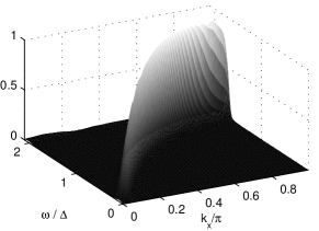
Figure 1: The Anderson-Bogoliubov phonon in an cubic lattice. The $x$-axis is the $x$-component of the momentum vector in the units of inverse lattice spacing, the $y$-axis is energy in the units of the pairing gap divided by $\hbar$, and the $z$-axis shows the dynamical structure factor from Eq. (28), in arbitrary units.

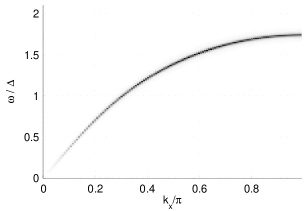
Figure 2: The dispersion of the Anderson-Bogoliubov phonon. The $x$-axis is the $x$-component of the momentum vector in the units of inverse lattice spacing and the the $y$-axis is energy in the units of the pairing gap divided by $\hbar$.

IV Speed of sound in a cubic 3D lattice

The density response in $(\mathbf{k},\omega)$ space (see Fig. 2) gives the dispersion of sound in the lattice. The long wavelength limit of the dispersion is linear and therefore the speed of sound is independent of momentum in that limit. For higher momenta the response saturates to $2\Delta$. In general the speed of sound in a weakly interacting Fermi gas is (to the leading order) $v_{F}/\sqrt{3}$, where $v_{F}$ is the Fermi velocity of the system. However, since the Fermi surface in a lattice is not a sphere, the Fermi velocity is not a uniquely defined number, but depends on the direction. With the definition

$$v_{Fx}=\frac{1}{\hbar}\left.\frac{d\epsilon_{\mathbf{k}}}{dk_{x}}\right|_{\mathbf{k}=k_{Fx}}=\frac{2J_{x}d}{\hbar}\sqrt{\left|\frac{E_{F}}{J_{x}}-\frac{1}{4}\left(\frac{E_{F}}{J_{x}}\right)^{2}\right|},$$ (29)

our results agree with the free space result in the low density limit.

In order to experimentally observe the density response in a finite system one must overcome some problems. In particular, the region of $\mathbf{k}$-space where the dispersion relation is linear scales with the inverse of the coherence length (or Cooper pair size) i.e. $\delta k\sim 1/\xi$. In the weakly interacting system, Cooper pairs become very large and the density response saturates very quickly to $2\Delta$. In the lattice the smallest non-zero wavevector has the magnitude of $k_{x}^{\text{min}}=2\pi/N_{x}\lambda$, where $N_{x}$ is the lattice size in the $x$-direction. This should be much smaller than the linear region of the dispersion. In other words the system size must be much larger than the coherence length. This leads to a condition for the minimum system size where the observation of density response is possible, which is shown in Fig. 3.

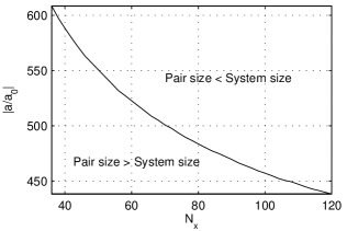
Figure 3: Pair size compared with the system size. The $x$-axis is the number of the lattice sites in the $x$-direction and the $y$-axis is the absolute value of the scattering length, in Bohr radii. For the density response to be experimentally observable, the coherence length, i.e. the size of a Cooper pair, must be smaller than the system. The linear sound dispersion is clearly visible above the solid line.

IV.1 Speed of sound and the van Hove singularity

Unlike in free space, in a lattice the speed of sound changes with the density of the atoms in a non-trivial way. Fig. 4 shows the speed as a function of the filling fraction with different interaction strengths. The sound velocity is typically on the order of ${\rm mm/s}$ and is thus experimentally measurable. With small scattering lengths and in a cubic lattice, the speed of sound as a function of the filling fraction is non-monotonous and exhibits a local minimum around the point where $E_{F}=4J$. For non-interacting fermions this minimum is a sharp cusp corresponding to the van Hove singularity in the density of states. The cusp appears when the Fermi surface in the direction of the sound reaches the divergence in the density of states. The cusp is visible in Fig. 4 where we show the isothermal sound velocity

$$c_{T}=\sqrt{\frac{\partial P}{\partial\rho}},$$ (30)

where $P$ is the pressure and $\rho$ is the mass density of the gas, calculated for the ideal Fermi gas in a finite sized lattice.

However, interactions smear the Fermi surface by broadening its edge by an amount of the pairing gap, $\Delta$. This smoothens out the cusp caused by the singularity. In fact, as is clear from the Fig. 4, the effect will vanish completely with strong enough interactions.

The finite size effects introduce some modulations, but it is clear that a non-zero gap shifts the minimum of the sound velocity into higher filling fractions. The non-zero gap also lowers the sound velocity and this effect becomes more pronounced at higher filling fractions. For a weakly interacting system with a very low filling fraction and an infinite lattice, the speed of sound is given by the analytical result Anderson (1958)

$$c=\frac{v_{F}}{\sqrt{3}}\sqrt{1+\frac{U(6\pi^{2}n)^{1/3}}{4\pi^{2}J_{x}d^{2}}}.$$ (31)

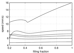
Figure 4: The speed of sound as a function of the lattice filling fraction, for the non-interacting Fermi gas (top curve) and for interacting Fermi gases with different scattering lenghts: (in Bohr radii, from top to bottom) $-750$, $-1000$, $-1200$, $-1500$, and $-2000$. The speed has a local minimum at a point where $E_{F}=4J$, but this minimum is smoothened out as interactions become stronger.

The location of the van Hove singularity is also the point where the Fermi surface of the system becomes disconnected in a non-interacting system. In the interacting case, the Fermi surface is smoothened, see Fig. 5.

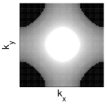
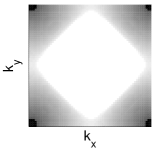
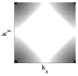
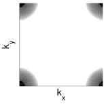
Figure 5: The Fermi surface of the lattice with different densities, as seen from the z-direction. The axis are the $x$- and $y$-components of the momentum vector. The surfaces above were plotted with filling fractions $0.2$, $0.44$, $0.47$, and $0.8$, from left to right. The colour coding: white corresponds to the Fermi surface reaching the edge of the Brillouin zone in the $z$-direction, whereas the black area is outside the surface. Note that the presence of the excitation gap spreads the Fermi surface, wheras for a non-interacting system, the edges of the Brillouin zone are not reached until the filling fraction exceeds 0.42.

IV.2 Speed of sound as a function of interaction strength

Increasing the interactions between atoms (i.e. increasing the scattering length) tends to reduce the sound velocity, as can be seen in Fig. 6. This behaviour is expected on the grounds that interaction strength increases the density of states in general, which increases the compressibility of the system, which in turn reduces the speed of sound. Note that in contrast, for a Bose-Einstein condensate with a positive scattering length the sound velocity actually increases as interactions become stronger.

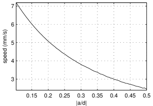
Figure 6: The speed of sound as a function of the scattering length $a$. Here $d$ is the lattice spacing, the filling fraction is $0.5$, and the lattice is cubic, with $s_{x},s_{y},s_{z}=2.5$.

V Non-cubic lattices and dimensional crossover

We now study density response and the speed of sound in non-cubic lattices. By varying the lattice heights $s_{x}$, $s_{y}$ and $s_{z}$, i.e. by changing the different laser intensities, the cubic symmetry of the lattice can be broken. For concreteness, we choose $s_{x}=s_{y}$. With this simplification, there are basically two distinct cases, namely $s_{x}>s_{z}$ and $s_{x}<s_{z}$. In the former case the atoms are more free to move in the $z$-direction than in the $xy$-plane. This means that the lattice resembles a square lattice arrangement of coupled one-dimensional tubes. The latter corresponds to a situation where movement is more restricted in the $z$-direction. In this case the lattice can thought to be a pile of connected two-dimensional planes (“pancakes”).

In either case, the energy gap $\Delta$, does not show any qualitative change when the symmetry decreases: $\Delta$ merely grows as either $s_{x}$ (and $s_{y}$) or $s_{z}$ is increased, since tighter confinement effectively increases interaction, see Fig. 7. However, there is a clear signal of a dimensional crossover in the speed of sound. In the two-dimensional limit, i.e. when the tunneling in the $z$-direction is suppressed (pancakes), the local minimum of the speed of sound vanishes, as can be seen from Fig. 8. Also it can be seen that the speed of sound is significantly larger in the direction parallel to the planes than orthogonal to them.

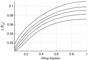
Figure 7: The energy gap as a function of the filling fraction with $s_{x}=s_{y}<s_{z}$, corresponding to quasi-two-dimensional pancakes along the $xy$-plane. The different curves are for different ratios of $s_{x}/s_{z}$: (from top to bottom) $0.5$, $0.62$, $0.71$, $0.83$, and $1.0$ (cubic case). There is no qualitative difference in the different curves. Here the scattering length $a$ is all the time $-1000a_{0}$.

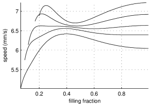
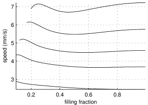
Figure 8: The speed of sound as a function of the lattice filling fraction in non-cubic lattices with $s_{x}=s_{y}<s_{z}$, corresponding to quasi-two-dimensional pancakes along the $xy$-plane. The left figure shows the speed in the plane, i.e. parallel to the pancakes, and the one on the right the speed orthogonal to the them, i.e. along the $z$-axis. The different curves are for different ratios of $s_{x}/s_{z}$: (from top to bottom) $1.0$ (cubic case), $0.83$, $0.71$, $0.62$, and $0.5$. Here the scattering length $a$ is all the time $-1000a_{0}$.

In the opposite case of stronger tunneling in the $z$-direction than in the $xy$-plane (1D tubes), the local minimum in the speed of sound also disappears. However, as is apparent from Fig. 9, in this one-dimensional limit the speed of sound is again qualitatively different from both the one in the three-dimensional cubic system and the one in the non-cubic system in the two-dimensional limit.

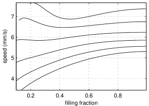
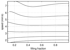
Figure 9: The speed of sound as a function of the lattice filling fraction in non-cubic lattices with $s_{x}=s_{y}>s_{z}$, corresponding to quasi-one-dimensional tubes along the $z$-axis. The figure on the left shows the speed in the $z$-direction, i.e. parallel to the tubes, and the right one the speed orthogonal to the them, i.e. in the $xy$-plane. The different curves are for different ratios of $s_{x}/s_{z}$: (from top to bottom) $1.0$ (cubic case), $1.2$, $1.4$, $1.6$, $1.8$, and $2.0$. Here the background scattering length $a$ is all the time $-1000a_{0}$.

VI Conclusions

In this paper, we have studied the velocity of sound in cubic and non-cubic three-dimensional optical lattices. We have investigated how the van Hove singularity of the free Fermi gas is smoothened by interactions and eventually vanishes when interactions are strong enough. In non-cubic lattices we have shown that although the energy gap has a simple behaviour as a function of symmetry, the speed of sound shows qualitatively different behaviour over the crossover, and provides a clear experimentally observable signature of a dimensional crossover both in the 1D and 2D limits.