Low temperature magnetization and the excitation spectrum of antiferromagnetic Heisenberg spin rings

Abstract

Accurate results are obtained for the low temperature magnetization versus magnetic field of Heisenberg spin rings consisting of an even number $N$ of intrinsic spins $s=1/2,1,3/2,2,5/2,3,7/2$ with nearest-neighbor antiferromagnetic (AF) exchange by employing a numerically exact quantum Monte Carlo method. A straightforward analysis of this data, in particular the values of the level-crossing fields, provides accurate results for the lowest energy eigenvalue $E_{N}(S,s)$ for each value of the total spin quantum number $S$. In particular, the results are substantially more accurate than those provided by the rotational band approximation. For $s\leq 5/2$, data are presented for all even $N\leq 20$, which are particularly relevant for experiments on finite magnetic rings. Furthermore, we find that for $s\geq 3/2$ the dependence of $E_{N}(S,s)$ on $s$ can be described by a scaling relation, and this relation is shown to hold well for ring sizes up to $N=80$ for all intrinsic spins in the range $3/2\leq s\leq 7/2$. Considering ring sizes in the interval $8\leq N\leq 50$, we find that the energy gap between the ground state and the first excited state approaches zero proportional to $1/N^{\alpha}$, where $\alpha\approx 0.76$ for $s=3/2$ and $\alpha\approx 0.84$ for $s=5/2$. Finally, we demonstrate the usefulness of our present results for $E_{N}(S,s)$ by examining the Fe₁₂ ring-type magnetic molecule, leading to a new, more accurate estimate of the exchange constant for this system than has been obtained heretofore.

I Introduction

Since the early 1990s, the field of magnetic molecules has blossomed, and the number of different species that exist is increasing rapidly.Sessoli et al. (1993); Gatteschi et al. (1994); Winpenny (2001, 2002, 2004) In particular, there is a large family of so-called ring-type magnetic moleculesWinpenny (2001); Taft et al. (1994); Abbati et al. (1997); Saalfrank et al. (1997); Watton et al. (1997); Atkinson et al. (1999); Caneschi et al. (1999); Abbati et al. (2000); Liu et al. (2001); McInnes et al. (2001); Chang et al. (2001); Dearden et al. (2001) that we focus on in the present work. Within such molecules there are embedded an even number $N$ of identical paramagnetic ions of intrinsic spin $s$ occupying $N$ equally-spaced sites defining a ring. Each such ion (“spin”) is coupled to its two nearest neighbors via an AF exchange interaction, resulting in systems that can oftenTaft et al. (1994); Abbati et al. (1997); Atkinson et al. (1999); Caneschi et al. (1999); Abbati et al. (2000); McInnes et al. (2001) be well represented by an isotropic Heisenberg model with a single exchange energy, $J>0$, of the form

$$\utilde{\mathcal{H}}=J\sum_{i=1}^{N}\utilde{\vec{s}}_{i}\cdot\utilde{\vec{s}}_{i+1}+g\mu_{B}\vec{H}\cdot\sum_{i=1}^{N}\utilde{\vec{s}}_{i},$$ (1)

where the spin operators $\utilde{\vec{s}}_{i}$ are given in units of $\hbar$, $g$ is the spectroscopic splitting factor, and $\mu_{B}$ is the Bohr magneton. In the first term of Eq. (1), the cyclic character of the system is maintained by requiring that $\utilde{\vec{s}}_{N+1}\equiv\utilde{\vec{s}}_{1}$. The second term describes the standard Zeeman effect, where the external field $\vec{H}$ is typically defined to be directed along the z-axis. The total spin operators $\utilde{S}^{2}$ and $\utilde{S}_{z}$ then commute with $\utilde{\mathcal{H}}$, and the eigenstates are described by quantum numbers $S$ and $M_{S}$ whose values range from $0$ to $Ns$ and from $-S$ to $S$, respectively. In Fig. 1 we display the zero-field energy spectrum corresponding to Eq. (1) for a particular example, $s=3/2$ and $N=6$, with the subset of minimal energies (SME) shown in red. The SME are closely related to what are called level-crossing fields, quantities which are used to study the SME in great detail throughout this work for many choices of $s$ and $N$.

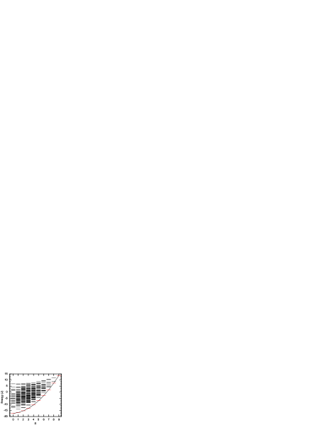
Figure 1: (Color online) Complete energy spectrum for $N=6$ and $s=3/2$ obtained by diagonalizing the Hamiltonain in Eq. (1) for $H=0$. The energy levels shown in red are the subset of minimal energies (SME) for this system as explained in the text. The solid line is a parabola, given in the text, that gives an excellent fit to the SME.

In an external magnetic field, the ($2S+1$)-fold degeneracy of each field-free multiplet is lifted due to a shift, $g\mu_{B}HM_{S}$, originating in the Zeeman term. As the external field is increased from $H=0$, the ground state will change (among the members of the zero-field SME) successively from $S=0$, $M_{S}=0$ to $S=1$, $M_{S}=-1$, etc., in integer steps of $S$ and $M_{S}$ until $S=-M_{S}=Ns$, corresponding to saturation of the magnetization. Each of the $Ns$ changes of the ground state quantum numbers is referred to as a level-crossing, and the field at which the $n$th level-crossing occurs is denoted in the following by $H_{n}$. By determining these fields, we seek to record the characteristics of the SME as a function of $s$ and $N$. This is accomplished using the difference equation,

$$E_{N}(S,s)=E_{N}(S-1,s)+g\mu_{B}H_{n}$$ (2)

for $S=n$, where $n$ extends from 1 to $Ns$. We elaborate on this connection between the SME and the $H_{n}$ in detail in the following section.

In order to appreciate the details of the SME, we first review some generic features of the spectra, and in particular the SME, that are already known. It has been noted,Abbati et al. (2000); Schnack and Luban (2000) and is clearly evident in Fig. 1, that the SME are accurately approximated by a quadratic dependence on $S$ of the form $E(S)\propto S(S+1)$, as for a quantum rotor. The solid curve in Fig. 1 describes the parabola $E(S)=cJS(S+1)/(2N)+E_{G}$, where $c=4.14$ gives the best fit to this SME which has a ground state energy $E_{G}=-17.393J$. [The reason for the inclusion of the factor of $2N$ in this equation will become clear in the next section.] If the SME were strictly parabolic in $S$, this would give rise to uniformly spaced level-crossing fields. Although uniform spacing is approximately realized in Fig. 2 for our example, we find that the accuracy of such an approximation deteriorates for larger values of $N$. This is explored in detail in Sec. II.

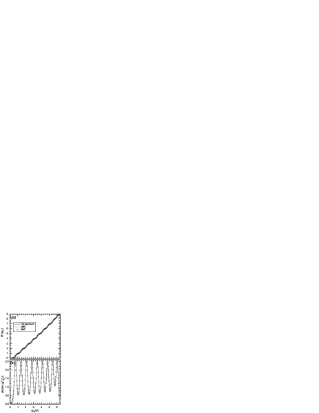
Figure 2: (Color online) (a) $M(H)$ and (b) $dM/dH$ for the example system ($N=6$ and $s=3/2$) at a fixed temperature, $k_{B}T/J=0.1$. The data in (b) are obtained by QMC calculations, and as a guide to the eye the line connects successive data points.

Above the SME there exists a large forest of energy levels. Although many of these levels lie very close to one another, there is a relatively large energy separation between the SME and the higher energy levels which has been previously observed.Schnack and Luban (2000); Waldmann (2001) Since at a low temperature $T$ only the lowest levels can be thermally occupied, and all other levels lie well above the SME, the magnetization as a function of field $M(H)$ consists of a series of thermally broadened steps that arise at the level-crossing fields and are determined solely by the SME. [The magnetization is also a function of $T$, but we will write $M(H)$ for the sake of brevity.] This step-like property is illustrated in Fig. 2, where $M(H)$ and $dM/dH$, the differential susceptibility, are shown for the $s=3/2$, $N=6$ example with $k_{B}T/J=0.1$. The data in Fig. 2(a) were calculated in three different ways: using the partition function that includes the complete energy spectrum; using the quantum Monte Carlo (QMC) method employed in this work; and using a modified partition function that includes only the states belonging to the SME. The sharp peaks that appear in Fig. 2(b) were calculated using QMC and the susceptibility fluctuation formula to give $dM/dH$ directly, not by differentiating $M(H)$.

The three data sets shown in Fig. 2(a) are all identical to 4 significant figures, supporting the assertion that the SME are sufficient for analyzing low temperature experimental data of this type. For larger values of $N$, lower temperatures are needed in order to obtain this degree of agreement, especially in the vicinity of the saturation field. For this reason, we have carefully checked that as the temperature is lowered the level-crossing fields have indeed converged to their limiting, temperature-independent values. As shown in Sec. II, it is these fields that are then used to calculate the SME function $E_{N}(S,s)$.

Despite the very simple appearance of the Hamiltonian of Eq. (1), the evaluation of the corresponding energy eigenvalues and resulting thermodynamic properties frequently presents a major challenge. The most straightforward way to deal with this Hamiltonian, and the method that is usually employed when analyzing magnetic molecules, is to numerically diagonalize the Hamiltonian matrix. This yields energy spectra such as that shown in Fig. 1. However, even for relatively small rings the dimensionality of the Hilbert space, given by $D=(2s+1)^{N}$, is so large that the exact diagonalization of the Hamiltonian matrix becomes totally impractical. For the small ring that has been considered as an example, $s=3/2$ and $N=6$ gives $D=4096$. If we consider a larger ring, for example $s=5/2$ and $N=12$ which will be analyzed in Sec. IV, we already have $D\approx 2.2\times 10^{9}$, which is well beyond the practical limit of existing computers. For $s=5/2$ and $N=20$, $D$ is a staggering $3.6\times 10^{15}$.

We can entirely avoid the obstacles confronting matrix diagonalization by using a QMC method that is not restricted by the dimensionality of the Hilbert space. We here only focus on low temperature $M(H)$ and $dM/dH(H)$ which are used to determine the SME, but other thermodynamic quantities such as the temperature dependent susceptibility, specific heat, and internal energy are also readily attainable using this method for all temperatures and fields, and are in fact computationally much less demanding than the present low temperature studies.

As seen above, knowledge of the SME enables one to obtain accurate values of low-temperature $M(H)$ and $dM/dH(H)$ data. To this end, the SME are calculated in Sec. II for all $s$ from 1/2 to 5/2 and all even $N$ from 4 to 20. These data are presented in the form of convenient, dimensionless “spectral coefficients” that will be introduced in that section. The spectral coefficients are also presented for larger rings, $N=40$, 80, and larger intrinsic spins, $s=3$ and $s=7/2$. Such large values of $N$ and $s$ have not yet, to our knowledge, been realized in magnetic molecules, but are useful for studying the approach to the classical limit ($s\to\infty$).

In Sec. III the energy gap $\Delta_{s}(N)$ between the $S=0$ ground state and the lowest $S=1$ state, which can be inferred from the first level-crossing field, is analyzed in greater detail for successively larger values of $N$, up to $N=50$, for $s=3/2,2,5/2$. This gap is experimentally relevant for NMR and INS experiments, and is also important for analyzing low temperature, low-field susceptibility data. Finally, as an illustration of the usefulness of the present results, in Sec. IV we analyze an existing ring-type magnetic moleculeCaneschi et al. (1999) composed of 12 Fe³⁺ ions ($s=5/2$), leading to an improved estimate for the exchange constant. With the experimental advancements that are being made both in the synthesis of molecules and in high field magnetization studies, we anticipate that the use of the theoretical data presented in this work will complement future experiments in a much needed way, providing more accurate estimates of microscopic parameters for future ring-type molecules.

II Spectral Coefficients

Since the Hilbert space associated with $\utilde{\mathcal{H}}$ is often too large to allow diagonalization of the Hamiltonian matrix, other theoretical methods must be found. To analyze low-field susceptibility data, classical spin models and scaled-up data from smaller systems can sometimes be useful.Taft et al. (1994); Caneschi et al. (1999); Abbati et al. (2000); McInnes et al. (2001) However, the level-crossings that are observed in high-field experiments have no classical analog and cannot be easily scaled up. For this reason, reliable theoretical data has previously been lacking, and a main goal of the current work is to remedy this situation through detailed QMC calculations.

In order to learn about the nature of the SME, we used the Stochastic Series Expansion methodSandvik and Kurkijarvi (1991); Syljuasen and Sandvik (2002) to simultaneously calculate both $M$ and $dM/dH$ versus $H$ at fixed temperatures, an example of which was shown in Fig. 2. From these data, we can very accurately infer the level-crossing fields and thereby reconstruct the SME. This follows from Eq. (2) which gives

$$E_{N}(S,s)=g\mu_{B}\sum_{n=1}^{S}H_{n}+E_{G},\qquad(1\leq S\leq Ns),$$ (3)

where $E_{G}\equiv E_{N}(0,s)$ is the ground state energy. It is convenient to define the quantities,

$$h_{n}\equiv\frac{g\mu_{B}H_{n}}{J}=\frac{c_{n}(N,s)n}{N},\qquad(n=1,\ldots,Ns),$$ (4)

where the dimensionless numbers $c_{n}(N,s)$ will be referred to as “spectral coefficients”. The energy spectrum of the SME may thus be written as

$$E_{N}(S,s)=\frac{J}{N}\sum_{n=1}^{S}nc_{n}(N,s)+E_{G},\qquad(1\leq S\leq Ns).$$ (3^′)

Note that if $c_{n}(N,s)$ were independent of $n$ and given by $c(N,s)$, Eq. (3^′) would reduce to

$$E_{N}(S,s)=\frac{c(N,s)J}{N}\frac{S(S+1)}{2}+E_{G},\qquad(0\leq S\leq Ns),$$ (5)

the so-called “rotational band” model that has often been employed to analyze magnetization data.Taft et al. (1994); Inagaki et al. (2003); Julien et al. (1999); Schnack and Luban (2000) Inspecting Eq. (4), the rotational band model immediately implies that the level-crossing fields are equally spaced which, as we will demonstrate in the subsequent subsections, is hardly the case. Instead, Eq. (3^′), in conjunction with the spectral coefficients presented in the following subsection, provides a highly accurate, yet convenient means of representing $E_{N}(S,s)$ and thus for analyzing low temperature magnetization data.

Based on previously known properties of Heisenberg rings, it is easy to show that $c_{n}(N,s)$ is exactly 4 for a very few special cases. These are listed here and will be useful in discussing the results of our calculations in subsequent subsections:

• In the case of the $N=4$ ring, $c_{n}(4,s)=4$, independent of $n$ and $s$. This is easily derived by describing this system in terms of two sublattices, each consisting of two spins. As a result, the SME is given exactly by $E_{4}(S,s)=JS(S+1)/2+E_{G}$.

• In the limit of classical spins,$\lim_{s\to\infty}c_{n}(N,s)=4$, for all $n$ and $N$.

• In all cases $c_{n=Ns}(N,s)=4$, independent of $N$ and $s$. This follows from Eq. (3^′) and the fact that the state with $S=Ns$ has energy $E_{N}(Ns,s)=JNs^{2}$, while the SME energy with $S=Ns-1$ is $E_{N}(Ns-1,s)=Js(Ns-4)$.Schmidt (2002)

Since the spectral coefficients have a value of exactly 4 both in the limit of very small rings (item I) and in the limit of very large intrinsic spins (item II), one might expect that the replacement, $c_{n}(N,s)=c(N,s)\approx 4$, independent of $n$, would provide a very good approximation, for example, for Fe³⁺ ions ($s=5/2$) in small rings ($N\leq 20$). However, as shown in the following subsections for different choices of $s$ and $N$, the spectral coefficients do vary significantly with $n$.

II.1 $s=1/2$, and $s=1$

Rings of $s=1/2$ spins have been studied using many methods, and a great deal is known about their spectra. In the 1960s, the lowest energies, $E_{N=\infty}(S,s=1/2)$, were calculatedGriffiths (1964) in the thermodynamic limit using the Bethe ansatz,Bethe (1931); Yang and Yang (1966) while numerical diagonalizationBonner and Fisher (1964) was carried out on finite rings. More recently, work has continued for finite $N$ using methods that include the quantum Monte CarloKashurnikov et al. (1999), renormalization groupWhite (1992); Wang and Xiang (1997), LanczosNightingale et al. (1993); Waldmann (2001) and conformal field theory methods.Affleck et al. (1989); Eggert et al. (1994)

The lowest eigenvalues for small $s=1/2$ rings can be easily obtained from straightforward matrix diagonalization, but are included here both for completeness and to assess the usefulness of Eqs. (3^′) and (5). The spectral coefficients that are shown in Fig. 3(a) as a function of $n/(Ns)$ define the SME for small $s=1/2$ rings. One can immediately notice that the $c_{n}$ vary with $n$, and most are much larger than 4, implying that a rotational band approximation provides a relatively poor approximation to these spectra.

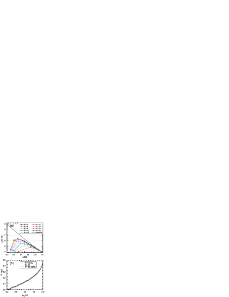
Figure 3: (Color online) (a) Spectral coefficients for small $s=1/2$ rings. The solid lines are included to guide the eye, and the continuous curve corresponds to the $N=\infty$ magnetization data of Ref. Griffiths, 1964. (b) $M(H)$ for $N=\infty$ (from Ref. Griffiths, 1964), for $N=20$ (QMC) and an approximation based on (7).

Also included in Fig. 3(a) are the spectral coefficients corresponding to Griffith’s original $M(H)$ result for the infinite $s=1/2$ chainGriffiths (1964) which is shown as a solid curve in Fig. 3(b). In the thermodynamic limit, the transformation from magnetization to spectral coefficients can be accomplished by making the replacement, $n/N\to m_{0}$, where $m_{0}$ is the zero temperature magnetization per spin in units of $g\mu_{B}$. Eq. (4) can then be rewritten,

$$c_{n}(N=\infty,s)=\frac{h_{n}}{m_{0}(h_{n})}.$$ (6)

As can be seen in Fig. 3(a), for $N=\infty$ the spectral coefficients form a nearly linear function of $n/(Ns)$ over a very large range of this variable. Approximating this data as a linear function,

$$c_{n}(N=\infty,1/2)\approx\alpha-\beta\frac{n}{Ns},$$ (7)

and substituting Eq. (7) into Eq. (6), again replacing $n/N\to m_{0}$, the resulting approximate magnetization is

$$m_{0}=\frac{\alpha s}{2\beta}\left(1-\sqrt{1-\frac{4\beta}{s\alpha^{2}}h}\right),$$ (8)

where $s=1/2$. Fitting the $c_{n}(\infty,1/2)$ data to the linear function, we find $\alpha=8.9$ and $\beta=5.07$. The corresponding curve terminates at the point ($h=1.953$, $m_{0}=0.439$), rather than at (2, 0.5), but otherwise is virtually indistinguishable in Fig. 3(b) from the exact magnetization (solid curve). This deviation of the terminus is due to the fact that the linear approximation of Eq. (7) does not incorporate a small positive curvature of the cluster coefficients as a function of $n/(Ns)$ as $n$ approaches $Ns$. Also included in Fig. 3(b) is $M(H)$ for the $s=1/2$, $N=20$ ring at a temperature $k_{B}T/J=0.05$. This data is nearly identical to that of the infinite ring, except for the existence of thermally broadened steps associated with level-crossings.

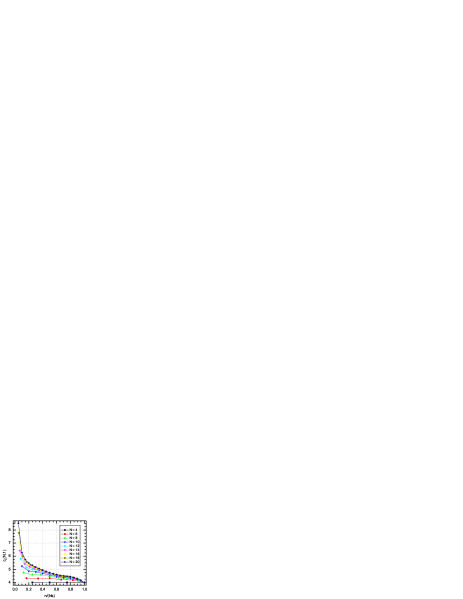
Figure 4: (Color online) Spectral coefficients for small rings of intrinsic spins $s=1$. The solid lines are included to guide the eye.

Heisenberg rings of $s=1$ spins have received a great deal of attention since Haldane’s predictionHaldane (1983) that a finite gap separates the ground state from the first excited state in infinite rings of integer spins $s$.Qin et al. (1997) In the notation of the present work, this gap is given by $\Delta_{s}(N)\equiv E_{N}(1,s)-E_{G}=\frac{J}{N}c_{1}(N,s)$, and the values of $c_{1}(N,1)$, seen as the left-most points in Fig. 4, are in good agreement with published valuesGolinelli et al. (1994) of $\Delta_{1}(N)$. Values of $\Delta_{s}(N)$ for all $s$ in the range $1/2\leq s\leq 5/2$ will be discussed in Sec. III.

Note however that the data presented here and in the next subsection include not only the first energy gap [associated with $c_{1}(N,s)$], but all energy levels that belong to the SME. Studying the details of of the SME, we find a very rich structure. For instance, it is evident in Fig. 4 that $c_{n}(N,1)$ decreases rapidly with increasing $n$, unlike the corresponding data for $s=1/2$. For $n\geq 0.4Ns$ the value of $c_{n}(N,1)$ has already fallen below 5 for $N\leq 20$, whereas for $s=1/2$ this value is not reached until $n>0.75Ns$. In this sense, increasing $s$ from 1/2 to 1 is a significant step on our way toward the classical limit, stated in item II of the previous section.

II.2 $s=3/2$, $s=2$ and $s=5/2$

Systems of larger intrinsic spins have also been studied in recent years,Parkinson and Bonner (1985); Schnack and Luban (2000); Waldmann (2001); Lou et al. (2002); Schnack (2000) but with less frequency than $s=1/2$ and $s=1$ systems. Since a knowledge of the spectral coefficients for $s=3/2$, 2 and 5/2 is important for a number of molecular rings, these data are presented in Fig. 5 for all $N\leq 20$. The values of $c_{1}(N,s)$ that appear in Figs. 5(a) and 5(b) agree with the values of $\Delta_{s}(N)$ that have been publishedSchnack (2000) ($N\leq 10$). Again, besides the first energy gap, the SME exhibit several interesting characteristics which are reflected in the spectral coefficients.

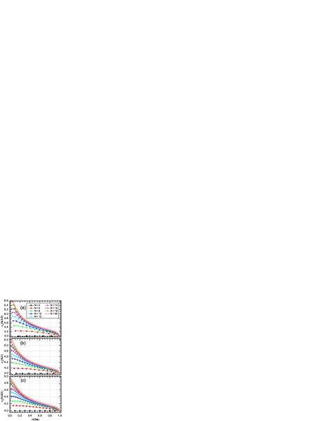
Figure 5: (Color online) Spectral coefficients for small rings of intrinsic spins $s=3/2,2,5/2$. The solid lines are included to guide the eye.

Of course, the spectral coefficients for $N=4$ are all equal to 4 as required by item I. As $N$ increases with fixed $s$ and $n/(Ns)$, the corresponding spectral coefficients increase from 4 monotonically, resulting in the series of nonintersecting curves seen in Fig. 5. This is consistent with Waldmann’s observationWaldmann (2001) that the rotational band model becomes poorer for larger rings.

Anchored at 4 for $n=Ns$ (item III), and always approaching 4 from above, the values of the spectral coefficients decrease sharply as $n$ approaches $Ns$. This ubiquitous drop can be discussed in a number of contexts. Recalling Eq. (4), this is clearly equivalent to a compression of the level-crossing fields as saturation is approached. At low temperatures this results in a large slope of $M(H)$, as can be seen in Fig. 6 for $N=20$ and $s=5/2$. In terms of the energy spectrum, this implies that the curvature of the SME decreases for large $S$.

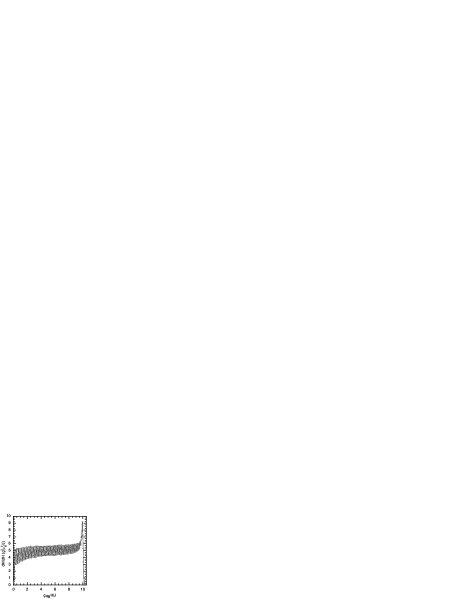
Figure 6: Differential susceptibility for a ring of $N=20$ intrinsic spins $s=5/2$ at a temperature, $k_{B}T/J=0.05$. The large peak immediately before saturation ($g\mu_{B}H/J=10$) is discussed in the text.

Finally, note that as $s$ is increased with fixed $N$ and $n/(Ns)$, the spectral coefficients descend toward 4 (item II), but only very slowly. Even for $s=5/2$, most of the spectral coefficients shown in Fig. 5(c) are considerably larger than 4, indicating that one is still far from the classical limit that is stated in item II. This behavior is explored in the next subsection with the inclusion of larger values of intrinsic spin.

II.3 Scaling relation for large $s$

Thus far we have presented the spectral coefficients that define the SME as a function of three variables, $s$, $N$, and $n/(Ns)$, and some general trends have emerged. Now, considering larger values of $s$ and $N$, we would like to make more quantitative statements regarding the functional dependence of $c_{n}(N,s)$ on these variables. To that end, we have calculated the spectral coefficients for values of $s$ up to 7/2 and present that data for $3/2\leq s\leq 7/2$.

In Fig. 7 we plot the quantity $[c_{n}(N,s)-4]\times s^{p}$ as a function of $n/(Ns)$ for the choice $p=1.05$. From these data the $s$ dependence of the spectral coefficients is immediately evident. For each value of $N$, the data for all $s$ lie on a single curve, implying that the spectral coefficients scale according to

$$c_{n}(N,s)=4+s^{-p}f(N,n/(Ns)).$$ (9)

In particular, for $s\to\infty$ Eq. (9) will be in accord with item II. The slow approach to 4 as $s$ is increased is noteworthy, as even $s=7/2$ is still far away from the classical limit. Choosing a slightly different value for the scaling exponent $p$, such as 1.03 or 1.07, yields visibly inferior results, so we conclude that $p=1.05\pm 0.01$.

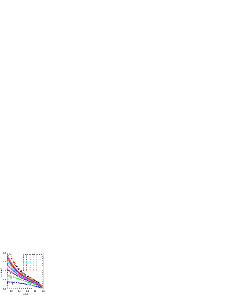
Figure 7: (Color online) Spectral coefficients adjusted to investigate the scaling behavior of Eq. (9) for all $s$ in the range $3/2\leq s\leq 7/2$. The data shown correspond to $p=1.05$.

A few of the spectral coefficients are also calculated for larger rings, $N=40$ and $N=80$. The inclusion of this data in Fig. 7 serves two purposes. First, this data suggests that $f(N,n/(Ns))$ is indeed converging to a finite limiting curve in the limit $N\to\infty$, which defines the zero temperature $M(H)$ of an infinite chain of spins $s$. Secondly, the larger $N$ data strengthens our belief that the scaling relation (9) is valid for all $N$.

Note that in Fig. 7 data are only included for $n/(Ns)>0.1$. The data for small $n/(Ns)$ have not been included because the error in calculating $c_{n}$ using the QMC method rapidly increases as $n/(Ns)$ decreases towards zero. The $n=1$ (gap) behavior is considered in the next section.

III Energy Gap

We now explore the energy gap $\Delta_{s}(N)$ between the ground state and the first excited SME level. Values of this gap are shown in Fig. 8(a) for rings of $N\leq 20$ spins $s\leq 5/2$. Much like the behavior of the full SME discussed in the previous section, this gap systematically approaches the limiting $s=\infty$ form as $s$ increases from $3/2$, while the $s=1/2$ and $s=1$ data exhibit distinctly different trends.

Specifically, the energy gap for $s=1/2$ rings is very similar to the energy gap that would be obtained for a ring with the same value of $N$ but very large $s$. This large $s$ limit, indicated in Fig. 8(a) as the “classical rotational band”, follows from item II and is given by $\Delta_{\infty}(N)=4J/N$. By contrast, $s=1$ rings have much larger gaps. Note also that these are already within 3.5% of the limiting, $N=\infty$ value even for $N=20$. The known limiting value,Qin et al. (1997) $\Delta_{1}(\infty)\approx 0.4105J$, is indicated by an arrow on the right side of Fig. 8(a).

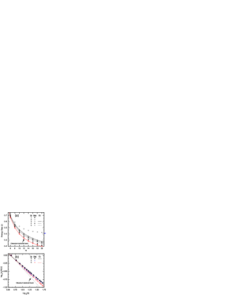
Figure 8: (Color online) Energy gap $\Delta_{s}(N)$ for rings of $N$ spins (a) for all $s\leq 5/2$ (symbols) along with the best fits to Eq. (10) (curves) as described in the text; and (b) with $N$ varying from 4 to 50 for $s=3/2$, 2, 5/2 (symbols) along with the best fits to Eq. (10) (lines) as described in the text.

Recall that for any $s$, $\Delta_{s}(4)=J$ from item I. Considering $N=6$, the classical result $\Delta_{\infty}(6)=2J/3$ is still a reasonable approximation to $\Delta_{s}(6)$, with a relative error of only a few percent for any $s$. However, as $N$ increases further this error continues to grow, and with $N=20$ it is nearly 25% for $s=5/2$ and nearly 40% for $s=3/2$.

Although the classical result is not sufficient, we find that the energy gaps for $s>1$ are well described by a slightly more general power law dependence on $N$ of the form

$$\Delta_{s}(N)\sim\Omega N^{-\alpha}.$$ (10)

The curves in Fig. 8(a) were obtained by choosing: $\Omega=2.68J$ and $\alpha=0.757$ for $s=3/2$; $\Omega=2.73J$ and $\alpha=0.781$ for $s=2$; $\Omega=3.03J$ and $\alpha=0.837$ for $s=5/2$; while of course $\Omega=4J$ and $\alpha=1$ corresponds to $s=\infty$. With these choices of $\Omega$ and $\alpha$, excellent agreement with the QMC data is obtained in the range $8\leq N\leq 20$, and it is clear that the classical limit is indeed being approached with increasing $s$ for both $\Omega$ and $\alpha$.

For the half odd integer spins, $s=3/2$ and $5/2$, the agreement with Eq. (10) continues for larger values of $N$. The same data are shown in Fig. 8(b), now including $N\leq 50$, and the QMC data agree with the power law formulas to within a fraction of a percent for all ring sizes in the range $8\leq N\leq 50$, which is comparable to our uncertainties in $\Delta_{s}(N)$. The values of $\Delta_{2}(N)$ begin to diverge from the power law dependence for $N\gtrsim 30$ which is to be expected since they must eventually converge to a non-zero value. This gap for $s=2$ chains has been previously studied in great detail, and density matrix renormalization group calculations have yielded a valueWang et al. (1999) of $\Delta_{2}(N)=0.0876J\pm 0.0013J$ in the limit as $N\to\infty$. One can see in Fig. 8(b) that $\Delta_{2}(N)$ is beginning to approach its limiting value, having become larger than $\Delta_{3/2}(N)$ for $N\geq 50$, but data for much larger rings would be necessary in order to obtain an accurate estimate for the limit $N\to\infty$.

The rotational band result, $\Delta_{s}(N)=4J/N$, has been used in the pastAbbati et al. (2000); Caneschi et al. (1999); Inagaki et al. (2003) as an estimate of $\Delta_{s}(N)$. Although this provides a reasonable approximation for $N<10$, as we have seen it quickly diverges from the correct result with increasing $N$. As such, it would be prudent to use the more accurate results presented here when attempting to relate $J$ to the experimentally measured lowest energy gap, e.g., by using INS, NMR, low-field susceptibility or magnetization data.

IV An application: Fe₁₂

In this section we apply our results to a known magnetic molecule,Caneschi et al. (1999) whose analysis has been challenged by a Hilbert space of dimension $D=6^{12}\approx 2.2\times 10^{9}$. The molecule is comprised of 12 Fe³⁺ ions ($s=5/2$), whose interaction was first investigatedCaneschi et al. (1999) by measuring the low-field susceptibility $\chi_{0}(T)$ as a function of temperature and fitting this data to an approximation of the $s=5/2$, $N=\infty$ chain. The exchange energy thus obtained was $J/k_{B}=31.9$ K for $g=2.00$. The field dependent magnetization of the molecule has also been measured and analyzed, and the first four level-crossing fields at low temperatures wereInagaki et al. (2003) $H_{1}=10.1\pm 0.2T$, $H_{2}=19.6\pm 0.2T$, $H_{3}=29.6\pm 0.4T$, $H_{4}=39.1\pm 0.8T$. An analysis of the magnetization was given in Ref. Inagaki et al., 2003 using the classical rotational band $c(N,s)=4$, and this yielded the estimate $J/k_{B}=40.7$ K with $g=2.02$. Note that the latter estimate is more than 25% larger than the formerCaneschi et al. (1999) estimate. Given the results of Sec. II, one can expect that the estimate $J=40.7$ K will be considerably larger than what will result from an accurate treatment of the Heisenberg model. This is borne out in the following.

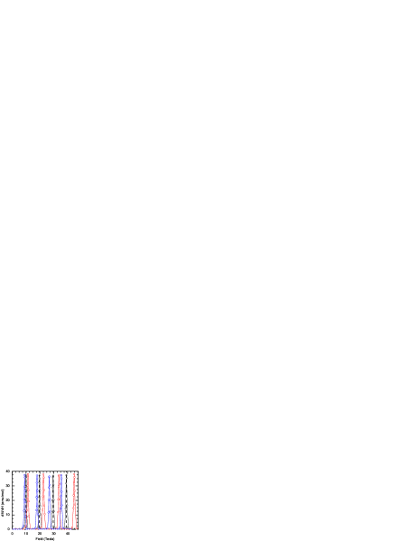
Figure 9: (Color online) The four measured level-crossing fieldsInagaki et al. (2003) (dashed vertical lines) are compared with the theoretical $dM/dH$ that result from $N=12$, $s=5/2$ Heisenberg rings with $k_{B}T/J=0.01$. The theoretical data are shown for the following three choices of $J$ and $g$: $J=31.9$ K and $g=2.00$ ( $\diamond$) from Ref. Caneschi et al., 1999; $J=40.7$ K and $g=2.02$ ( $\Box$) from Ref. Inagaki et al., 2003; $J=35.2$ K and $g=2.0$ ($\circ$) are our best estimates.

Figure 10: The first four spectral coefficients for the $N=12$, $s=5/2$ ring ($\times$) along with their errors bars, compared with the results of inserting the first four level-crossing fields and uncertainties from Ref. Inagaki et al., 2003 into Eq. (4) with the choice, $J/(k_{B}g)=17.6$ K ($\circ$).

In Fig. 9 we compare the four measured level-crossing fields with our low temperature ($k_{B}T/J=0.01$) QMC results. At this low temperature, each level-crossing of the theoretical $s=5/2$, $N=12$ Heisenberg ring is clearly indicated by a narrow peak in $dM/dH$. Note that the peaks in the QMC data arising from the parameters $J=31.9$ K and $g=2.00$ occur at fields that are considerably below the experimental level-crossings indicated by the dashed vertical lines. On the other hand, the QMC peaks that correspond to $J=40.7$ K and $g=2.02$ are all at fields significantly greater than the measured values. Particularly at high fields, these discrepancies become quite pronounced, suggesting that neither choice of parameters is consistent with the experimental data. However, we find that the predictions of the Heisenberg model agree very well with the experimental data if we use $J=35.2$ K and $g=2.0$. With this choice of parameters, each of the four theoretical peaks clearly coincides with a measured level-crossing shown in Fig. 9.

Without using the $dM/dH$ level-crossing field data directly, one can easily arrive at the same estimate based on the spectral coefficients of Sec. II. Recalling Eq. (4), the ratio of $J$ to $g$ is given by $J/g=N\mu_{B}H_{n}/[nc_{n}(N,s)]$. An estimate of this ratio for a given molecule is then obtained by simply inserting a measured value of $H_{n}$ and the corresponding $c_{n}(N,s)$ from Fig. 5.

Alternatively, from the measured $H_{n}$ we can construct an experimental analog of the spectral coefficients by fixing the ratio $J/g$ in Eq. (4). In Fig. 10 we display those results for the four measured $H_{n}$ (and their uncertainties). These data are in good agreement with the spectral coefficients if we choose the ratio $J/(k_{B}g)=17.6$ K, consistent with our previously stated estimate.

A small decrease with increasing $n$ is observable in the spectral coefficients derived from the experimental values of the level-crossing fields. This is expected from the data presented in Sec. II, but more level-crossings and/or smaller experimental error bars are needed in order to clarify this point. These data are also useful for getting a sense of the typical errors in the spectral coefficients that were presented in Sec. II. As shown in Fig. 10, the error bars of the QMC data decrease very rapidly with increasing $n$ and are in fact not visible in Figs. 5 and 7.

Our conclusion is that the existing data for the Fe₁₂ molecule is best fit by the choice $g=2.0$, $J=35.2$ K. This value of $J$ is 13.5% smaller than the value that resultedInagaki et al. (2003) from analyzing the experimental level-crossing fields using c(N,s) = 4. This reflects the fact that the spectral coefficients, although not constant, exceed 4 by approximately 13%. A similar analysis would be equally straightforward for any other rings whose spectral coefficients are shown in Sec. II.

V Summary

In this article we have utilized a quantum Monte Carlo (QMC) methodSandvik and Kurkijarvi (1991); Syljuasen and Sandvik (2002) to calculate detailed properties of the general quantum Heisenberg ring. This system consists of an even number $N$ of equally-spaced spins $s$ mounted on a ring, where the spins interact via nearest-neighbor antiferromagnetic isotropic exchange, with a single exchange constant $J$. As this system does not exhibit magnetic frustration it was possible to calculate thermodynamic quantities down to very low temperatures. In this work our primary focus has been on the accurate determination of the level-crossing fields, which in turn directly provide the lowest energy eigenvalue $E_{N}(S,s)$ for each value of the total spin quantum number $S$. By introducing the notation of spectral coefficients [see Eq. (4)], denoted by $c_{n}(N,s)$, we obtained an especially convenient representation of $E_{N}(S,s)$, given by Eq. (3^′). As the QMC method operates without diagonalizing the Hamiltonian matrix, we were able to obtain results for spins $s=1/2$, 1, 3/2, 2, 5/2, 3, 7/2, focusing mostly on $N\leq 20$ as these are experimentally relevant, although $N\leq 80$ were also considered. Among our principal results, we have found that the set of level-crossing fields are not uniformly spaced, and thus the spectral coefficients $c_{n}(N,s)$ vary significantly with $n$. Equivalently, $E_{N}(S,s)$ departs from the strictly quadratic dependence on $S$, referred to as the rotational band approximationSchnack and Luban (2000) (equivalently, the Land$\acute{e}$ interval rule). These deviations from uniform spacing are fairly small for $N\leq 8$, however, they become increasingly severe with increasing $N$. Similarly, the ground state energy gap, which may be written as $\Delta_{s}(N)=E_{N}(1,s)-E_{N}(0,s)=c_{1}(N,s)J/N$, varies significantly with $N$ and $s$. For $s=1$, 2 we find that, consistent with the Haldane result,Haldane (1983) $\Delta_{s}(N)$ is indeed converging to a non-zero limiting gap for large $N$, and in good agreement with estimates in the literatureQin et al. (1997); Wang et al. (1999) for these two choices of $s$. By contrast, for $s=3/2$, 5/2 we find that $\Delta_{s}(N)$ appears to decrease to zero for large $N$ according to a power law, [see Eq. (10)], where the exponent is given by $\alpha\approx 0.76$ for $s=3/2$ and $\alpha\approx 0.84$ for $s=5/2$. The increase with $\alpha$ towards unity with increasing $s$ is consistent with the known rigorous result,Schmidt and Luban (2003) $\Delta_{\infty}(N)=4J/N$, for the classical Heisenberg ring, which may be pictured as the quantum Heisenberg ring in the limit $s\to\infty$. We also find that the departure of the general spectral coefficient $c_{n}(N,s)$ from the classical result $c_{n}(N,\infty)=4$ is characterized by power law behavior [see Eq. (9)]. Finally, we have illustrated the practical utility of our present results for the level-crossing fields and $E_{N}(S,s)$ by considering the ring-type magnetic molecule knownCaneschi et al. (1999) as Fe₁₂. In particular, our analysis of the existingInagaki et al. (2003) experimental data for level-crossing fields shows that this system can be very well described by the nearest-neighbor Heisenberg model with antiferromagnetic exchange, and we are able to provide a new and improved estimate of the exchange constant. Although only rings with even $N$ have been considered in this work, we suspect that similar scaling relations may hold for other structures as well.