Euclidean random matrices: solved and open problems

Abstract

In this paper I will describe some results that have been recently obtained in the study of random Euclidean matrices, i.e. matrices that are functions of random points in Euclidean space. In the case of translation invariant matrices one generically finds a phase transition between a phonon phase and a saddle phase. If we apply these considerations to the study of the Hessian of the Hamiltonian of the particles of a fluid, we find that this phonon-saddle transition corresponds to the dynamical phase transition in glasses, that has been studied in the framework of the mode coupling approximation. The Boson peak observed in glasses at low temperature is a remanent of this transition. We finally present some recent results obtained with a new approach where one deeply uses some hidden supersymmetric properties of the problem.

1 Introduction

In the last years many people have worked on the problem of analytically computing the properties of Euclidean random matrices [2]-[16]. The problem can be formulated as follows.

We consider a set of $N$ points ($x_{i}$) that are randomly distributed with some given distribution.Two extreme examples are:

• The $x$’s are random independent points with a flat probability distribution, with density $\rho$.

• The $x$’s are one of the many minima of a given Hamiltonian.

In the simplest case of the first example, given a function $f(x)$, we consider the $N\times N$ matrix:

$$M_{i,k}=f(x_{i}-x_{k})\ .$$ (1)

The problem consists in computing the properties of the eigenvalues and of the eigenvectors of $M$. Of course, for finite $N$ they will depend on the instance of the problem (i.e. the actually choice of the $x$’s), however system to system fluctuations for intensive quantities (e.g. the spectral density $g(z)$) disappear when we consider the limit $N\to\infty$ at fixed particle density $\rho$.

The problem is not new; it has been carefully studied in the case where the positions of the particles are restricted to be on a lattice [17]. The case where the particles can stay in arbitrary positions, that is relevant in the study of fluids, has been less studied, although in the past many papers have been written on the argument [2]-[16]. These off-lattice models present some technical (and also physical) differences with the more studied on-lattice models.

There are many possible physical motivations for studying these models, that may be applied to electronic levels in amorphous systems, very diluted impurities, spectrum of vibrations in glasses (my interest in the subject comes from this last field).

I will concentrate in these lectures on the spectral density and on the Green functions, trying to obtaining both the qualitative features of these quantities and to present reasonable accurate computations (when possible). This task is not trivial because there is no evident case that can be used as starting point for doing a perturbation expansion. Our construction can be considered as a form of a mean field theory (taking care of some corrections to it): more sophisticated problems, like localization or corrections to the naive critical exponents will be only marginally discussed in these notes.

A certain number of variations to equation (1) are interesting. For example we could consider the case where we add a fluctuating term on the diagonal:

$$M_{i,k}=\delta_{i,k}\sum_{j}f(x_{i}-x_{j})-f(x_{i}-x_{k})\ .$$ (2)

This fluctuating diagonal term has been constructed in such a way that

$$\sum_{k}M_{i,k}=0\ .$$ (3)

Therefore the diagonal and the off-diagonal matrix elements are correlated.

In general it may be convenient to associate a quadratic form to the matrix $M$: the quadratic form (${\cal H}[\phi]$) is defined as:

$${\cal H}[\phi]=\frac{1}{2}\sum_{i,k}\phi_{i}\phi_{k}M_{i,k}\ .$$ (4)

In the first case we considered, eq. (1), we have that:

$${\cal H}[\phi]=\sum_{i,k}f(x_{i}-x_{k})\phi_{i}\phi_{k}\ .$$ (5)

In this second case, eq. (2), the associated quadratic form is given by

$${\cal H}[\phi]=\sum_{i,k}\phi_{i}\phi_{k}M_{i,k}=\frac{1}{2}\sum_{i,k}f(x_{i}-x_{k})(\phi_{i}-\phi_{k})^{2}\ .$$ (6)

Here the matrix $M$ is non-negative if the function $f$ is non-negative. The matrix $M$ has always a zero eigenvalue as consequence of the invariance of the quadratic form under the symmetry $\phi_{i}\to\phi_{i}+\lambda$; the presence of this symmetry has deep consequences on the properties of the spectrum of $M$ and, as we shall see later, phonons are present. Many of the tricky points in the analytic study are connected to the preserving and using this symmetry in the computations.

In the same spirit we can consider a two-body potential $V(x)$ and we can introduce the Hamiltonian

$$H[x]=\frac{1}{2}\sum_{i,k}V(x_{i}-x_{k})\ .$$ (7)

We can construct the $3N\times 3N$ Hessian matrix

$$M_{i,k}={\partial^{2}H\over\partial x_{i}x_{k}}=\delta_{i,k}\sum_{j}V^{\prime\prime}(x_{i}-x_{j})-V^{\prime\prime}(x_{i}-x_{k})\ ,$$ (8)

where for simplicity we have not indicated space indices. Also here we are interested in the computation of the spectrum of $M$. The translational invariance of the Hamiltonian implies that the associated quadratic form is invariant under the symmetry $\phi_{i}\to\phi_{i}+\lambda$ and a phonon-like behavior may be expected.

This tensorial case, especially when the distribution of the $x$’s is related to the potential $V$, is the most interesting from the physical point of view (especially for its mobility edge [17, 16]). Here we stick to the much simpler question of the computation of the spectrum of $M$. We shall develop a field theory for this problem, check it at high and low densities, and use a Hartree type method.

Our aim is to get both a qualitative understanding of the main properties of the spectrum and of the eigenvalues and a quantitate, as accurate as possible, analytic evaluation of these properties. Quantitative accurate results are also needed because the computation of the spectral density is a crucial step in the microscopic computation of the thermodynamic and of the dynamic properties of glass forming systems. In some sense this approach can be considered as an alternative route to obtain mode-coupling like results [18], the main difference being that in the mode coupling approach one uses a coarse grained approach and the hydrodynamical equations, while here we take a fully microscopic point of view.

Many variations can be done on the distribution of points, each one has its distinctive flavor:

• The distribution of the points $x$ is flat and the points are uncorrelated: they are uniformly distributed in a cube of size $L$ and their number is $N=\rho L^{3}$. Here, as in the following cases, we are interested in the thermodynamic limit where both $L$ and $N$ go to infinity at fixed $\rho$.

• The points $x$ are distributed with a distribution that is proportional to $\exp(-\beta H[x])$ where $H[x]$ is a given function.

• The points $x$ are one of the many solutions of the equation $\partial H/\partial x_{i}=0$. This last problem may be generalized by weighting each stationary point of $H$ with an appropriate weight.

The last two cases are particularly interesting when

$$M_{i,k}={\partial^{2}H\over\partial x_{i}x_{k}}\ ,$$ (9)

and consequently

$${\cal H}[\phi]=\frac{1}{2}\sum_{i,k}\phi_{i}\phi_{k}{\partial^{2}H\over\partial x_{i}x_{k}}\ .$$ (10)

If this happens the distribution of points and the matrix are related and the theoretical challenge is to use this relation in an effective way.

In the second section of these lectures, after the introduction we will present the basic definition of the spectrum, Green functions, structure functions and related quantities. In the third section we will discuss the physical motivation for this study and we will present a first introduction to the replica method. In the fourth section we will give a few example how a field theory can be constructed in such way that it describes the properties of randomly distributed points. In the fifth section we will discuss in details the simples possible model for random Euclidean matrices, presenting both the analytic approach and some numerical simulations. In the sixth section we shall present a similar analysis in a more complex and more physically relevant case, where phonons are present due to translational invariance. Finally, in the last section we present some recent results that have been obtained in the case of correlated points.

2 Basic definitions

The basic object that we will calculate are the matrix element of the resolvent

$$G[x](z)_{i,j}=\left(\frac{1}{z-M[x]}\right)_{ij}\ ,$$ (11)

(we use the notation $M[x]$ in order to stress that the matrix $M$ depends on all the points $[x]$. Sometimes we will suppress the specification “$[x]$”, where it is obvious. We can define the sample dependent Green function

$$G[x](y_{1},y_{2},z)=\sum_{i,j}\delta(y_{1}-x_{i})\delta(y_{2}-x_{j})G[x](z)_{i,j}=$$

$$\sum_{i,j}\delta(y_{1}-x_{i})\delta(y_{2}-x_{j})\left(\frac{1}{z-M[x]}\right)_{ij}\ .$$ (12)

The quantity that we are interested to compute analytically are the sample averages of the Green function, i.e.

$$\overline{G}(y_{1},y_{2},z)=\overline{G[x](y_{1},y_{2},z)}\,,$$ (13)

where the overline denotes the average over the random position of the points.

If the problem is translational invariant, after the average on the positions of the points $[x]$ we have

$$\overline{G}(y_{1},y_{2},z)=\overline{G}(y_{1}-y_{2},z)\ ,$$ (14)

where the function $\overline{G}(x,z)$ is smooth apart from a delta function at $x=0$. It is convenient to consider the Fourier transform of $\overline{G}(x,z)$, i.e.

$$G(p,z)={1\over N}\overline{\sum_{ij}e^{ip(x_{i}-x_{j})}\left[\frac{1}{z-M}\right]_{ij}}=$$

$${1\over N}\overline{\int dxdye^{ip(x-y)}G[x](x,y,z)}=\int dxe^{ipx}\tilde{G}(x,z)\ ,$$ (15)

The computation of the function $G(p,z)$ will one of the main goals of these lectures. It is convenient to introduce the so called dynamical structure factor (that in many case can be observed experimentally) that here is defined as :

$$S_{e}(p,E)=-\frac{1}{\pi}\lim_{\eta\to 0^{+}}G(p,E+{\mathrm{i}}\eta)\ .$$ (16)

One must remember that the structure function is usually defined using as variable $\omega=\sqrt{E}$:

$$S(p,\omega)=2\omega S_{e}(p,\omega^{2})\,,$$ (17)

The resolvent will also give us access to the density of states of the system:

$$g_{e}(E) = -\frac{1}{N\pi}\lim_{\eta\to 0^{+}}\overline{\sum_{i=1}^{N}\left[\frac{1}{E+{\mathrm{i}}\eta-M}\right]_{ii}}\,,$$ (18)

$$= -\frac{1}{\pi}\lim_{\eta\to 0^{+}}\lim_{p\to\infty}G(p,E+{\mathrm{i}}\eta)\,.$$

3 Physical motivations

There are many physical motivations for studying these problems, apart from the purely mathematical interest. Of course different applications will lead to different forms of the problems. In this notes I will concentrate my attention on the simplest models, skipping the complications (that are not well understood) of more complex and interesting models.

3.1 Impurities

We can consider a model where there are some impurities in a solid that are localized at the points $x$’s. There are many physical implementation of the same model; here we only present two cases:

• There may be electrons on the impurities and the amplitude for hopping from an impurity ($i$) to an other impurity ($k$) is proportional to $f(x_{i}-x_{k})$. The electron density is low, so that the electron-electron interaction can be neglected.

• There is a local variable $\phi_{i}$ associated to the impurity (e.g. the magnetization) and the effective Hamiltonian at small magnetizations is given by eq.(5).

In both cases it is clear that the physical behavior is related to the properties of the matrix $M$ that is of the form discussed in the introduction. If the concentration of the impurities is small (and the impurities are embedded in an amorphous system) the positions of the impurities may be considered randomly distributed in space.

3.2 Random walks

Let us assume that there are random points in the space and that there is a particle that hops from one point to the other with probability per unit time given by $f(x_{i}-x_{k})$.

The evolution equation for the probabilities of finding a particle at the point $i$ is given by

$${dP_{i}\over dt}=\sum_{k}f(x_{i}-x_{k})P_{k}-P_{i}\sum_{k}f(x_{i}-x_{k})=-\sum_{k}M_{i,k}P_{k}\,,$$ (19)

where the matrix $M$ is given by eq. (2).

Let us call $P(x,t)$ the probability that a particle starting from a random point at time 0 arrives at at time $t$. It is evident that after averaging of the different systems (or in a large system after averaging over the random starting points) we have that

$$\int_{0}^{\infty}dt\exp(-tz)\int dx\exp(ipx)P(x,t)=-G(p,-z)\,,$$ (20)

so that the function $P(x,t)$ can be reconstructed from the knowledge of the function $G(p,z)$ defined in eq. (15).

3.3 Instantaneous modes

We suppose that the points $x$’s are distributed according to the probability distribution

$$\exp(-\beta H[x])\ ,$$ (21)

where $H[x]$ is for example a two body interaction given by eq.(7) and $\beta=1/(kT)$.

The eigenvectors of the Hessian of the Hamiltonian (see eq.(8)) are called instantaneous normal modes (INN). The behavior of the INN at low temperature, especially for systems that have a glass transition [21, 20], is very interesting [22]. In particular there have been many conjectures that relate the properties of the spectrum of INN to the dynamic of the system when approaching the glass transition.

However it has been realized in these years that much more interesting quantities are the instantaneous saddle modes (ISN) [23, 24, 26, 25]. Given an equilibrium configuration $x_{e}$ at temperature $T$ one defined the inherent saddle $x_{s}$ corresponding to that configuration $x_{e}$ in the following way. We consider all the saddles of the Hamiltonian, i.e. all the solutions of the equations

$${\partial H\over\partial x_{i}}=0\,.$$ (22)

The inherent saddle $x_{s}$ is the nearest saddle to the configuration $x_{e}$. The Boltzmann distribution at temperature $T$ induces a probability distribution on the space of all saddles. The physical interesting quantities are the properties of the Hessian around these saddles. It turns out that they have a very interesting behavior near the glass transition in the case of glass forming materials.

It is clear that the computation of the spectrum in these case is much more complex: we have both to be able to compute the correlations among the points in this non-trivial case and to take care of the (often only partially known) correlations.

A possible variation on the same theme consists in consider the ensemble of all saddles of given energy $E=H[x]$: there are indications that also in this case there may be a phase transition in the properties of the eigenvalues and eigenvectors when $E$ changes and this phase transition may be correlated to some experimentally measured properties of glassy systems, i.e. the Boson Peak, as we will see later.

4 Field theory

4.1 Replicated Field Theory

The resolvent $G(p,z)$ defined in eq.(15) can be written as a propagator of a Gaussian theory:

$${\cal Z}[J] \equiv \int{\prod_{k}d\phi_{k}\exp\left(-{1\over 2}\sum_{lm}\phi_{l}\left(z-M\right)_{lm}\phi_{m}+\sum_{l}\phi_{l}J_{l}\right)}\,,$$

$$G(p,z) = {1\over N}\sum_{ij}\frac{\delta^{2}}{\delta J_{i}\delta J_{j}}\left.\overline{\exp(ip(x_{i}-x_{j}))\ln{\cal Z}[J]\>}\right|_{J=0}\,,$$ (23)

where the overline denotes the average over the distribution $P[x]$ of the positions of the particles. We have been sloppy in writing the Gaussian integrals (that in general are not convergent): one should suppose that the $\phi$ integrals go from $-a\infty$ to $+a\infty$ where $a^{2}=-i$ and $z$ has a positive (albeit infinitesimal) imaginary part in order to make the integrals convergent [17, 19]. This choice of the contour is crucial for obtaining the non compact symmetry group for localization [19], but it is not important for the density of the states.

In other words, neglecting the imaginary factors, we can introduce a probability distribution over the field $\phi_{i}$,

$$P[\phi]\propto\ \prod_{k}d\phi_{k}\exp\left(-{1\over 2}\sum_{lm}\phi_{l}\left(z-M\right)_{lm}\phi_{m}\right)\ .$$ (24)

If we denote by $\langle\cdot\rangle$ the average with respect to this probability (please notice that here everything depends on $[x]$ also if this dependence is not explicitly written) we obtain the simple result:

$$\langle\phi_{i}\phi_{k}\rangle=\ G_{i,k}\ .$$ (25)

A problem with this approach is that the normalization factor of the probability depends on $[x]$ and it is not simple to get the $x$-averages of the expectation values. Replicas are very useful in this case. They are an extremely efficient way to put the dirty under a simple carpet (on could also use the supersymmetric approach of Efetov where one puts the same dirty under a more complex carpet [17]).

For example the logarithm in eq.(23) is best dealt with using the replica trick [2, 3, 26]:

$$\ln{\cal Z}[J]=\lim_{n\to 0}\frac{1}{n}\left({\cal Z}^{n}[J]-1\right)\,.$$ (26)

The resolvent can then be computed from the $n$-th power of ${\cal Z}$, that can be written using $n$ replicas, $\phi^{(a)}_{i}$ ($a=1,2,\ldots,n$) of the Gaussian variables of eq.(23):

$$G(p,z)=\lim_{n\to 0}G^{(n)}(p,z)\ ,$$

$$NG^{(n)}(p,z)=$$ (27)

$$\sum_{ij}\overline{\exp(ip(x_{i}-x_{j}))\int\prod_{k,a}d\phi^{(a)}_{k}\,\phi^{(1)}_{i}\phi^{(1)}_{j}\,\exp\left(-{1\over 2}\sum_{l,m,c}\phi^{(c)}_{l}\left(z-M\right)_{lm}\phi^{(c)}_{m}\right)}\,.$$

Indeed

$$\int\prod_{k,a}d\phi^{(a)}_{k}\,\phi^{(a)}_{i}\phi^{(b)}_{j}\,\exp\left(-{1\over 2}\sum_{l,m,c}\phi^{(c)}_{l}\left(z-M\right)_{lm}\phi^{(c)}_{m}\right)\propto\delta_{a,b}=$$

$$\left[{1\over z-M}\right]_{i,j}\det(z-M)^{-n/2}$$ (28)

and the physically interesting case is obtained only when $n=0$.

In this way one obtains a $O(n)$ symmetric field theory. It well known that an $O(n)$ symmetric theory is equivalent to an other theory invariant under the $O(n+2|1)$ symmetry ([27]), where this group is defined as the one that leaves invariant the quantity

$$\sum_{a=1,n+2}(\phi^{a})^{2}+\bar{\psi}\psi\,,$$ (29)

where $\psi$ is a Fermionic field. Those who hate analytic continuations, can us the group $O(2|1)$ at the place of the more fancy $O(0)$ that is defined only as the analytic continuation to $n=0$ of the more familiar $O(n)$ groups.

Up to this point everything is quite general. We still have to do the average over the random positions. This can be done in an explicit or compact way in some of the previous mentioned cases and one obtains a field theory that can be studied using the appropriate approximations. Before doing this it is may be convenient to recall a simpler result, i.e. how to write a field theory for the partition function of a fluid.

4.2 The partition function of a fluid

Let us consider a system with $N$ (variable) particles characterized by a classical Hamiltonian $H_{N}[x]$ where the variable $x$ denote the $N$ positions. In the simplest case the particles can move only in a finite dimensional region (a box $B$ of volume $V_{B}$) and they have only two body interactions:

$$H_{N}[x]=\frac{1}{2}\sum_{i,k}V(x_{i}-x_{k})\ .$$ (30)

At given $\beta$ the canonical partition function can be written as

$${\cal Q}_{N}=\int_{B}dx_{1}\ldots dx_{N}\exp(-\beta H_{N}[x])\ ,$$ (31)

while the gran-canonical partition function is given by

$${\cal Q}(\zeta)=\sum_{N}{\zeta^{N}\over N!}{\cal Q}_{N}\ ,$$ (32)

where $\zeta$ is the fugacity.

We aim now to find out a field theoretical representation of the ${\cal Q}(\zeta)$. This can be formally done [29] (neglecting the problems related to the convergence of Gaussian integrals) by writing

$$\exp\left(-\frac{\beta}{2}\sum_{i,k}V(x_{i}-x_{k})\right)=$$

$${\cal N}^{-1}\int d\sigma\exp\left(\frac{1}{2\beta}\int dxdyV^{-1}(x-y)\sigma(x)\sigma(y)+\sum_{i}\sigma(x_{i})\right)\ ,$$ (33)

where ${\cal N}$ is an appropriate normalization factor such that

$${\cal N}^{-1}\int d\sigma\exp\left(\frac{1}{2\beta}\int dxdyV^{-1}(x-y)\sigma(x)\sigma(y)+\int J(x)\sigma(x)\right)=$$

$$\exp\left(-\int dxdy\beta V(x-y)J(x)J(y)\right)\ .$$ (34)

The reader should notice that $V^{-1}(x-y)$ is formally defined by the relation

$$\int dzV^{-1}(x-z)V(z-y)=\delta(x-y)\ .$$ (35)

The relation eq.(33) trivially follows from the previous equations if we put

$$J(x)=\sum_{i}\delta(x-x_{i})\ .$$ (36)

It is convenient to us the notation

$$d\mu[\sigma]\equiv{\cal N}^{-1}d\sigma\exp\left(\frac{1}{2\beta}\int dxdyV^{-1}(x-y)\sigma(x)\sigma(y)\right)\ .$$ (37)

With this notation we find

$${\cal Q}_{N}=\int d\mu[\sigma]\left(\int dx\exp(\sigma(x)\right)^{N}\ .$$ (38)

We finally get

$${\cal Q}(\zeta)=\int d\mu[\sigma]\exp\left(\zeta\int dx\exp(\sigma(x))\right)\ .$$ (39)

People addict with field theory can use this compact representation in order to derive the virial expansion, i.e. the expansion of the partition in powers of the fugacity at fixed $\beta$.

The same result can be obtained in a more straightforward way [30] by using a functional integral representation for the delta function:

$$\exp\left(-\frac{\beta}{2}\sum_{i,k}V(x_{i}-x_{k})\right)=$$

$$\int d[\rho]\delta_{F}\left[\rho(x)-\sum_{i=1,N}\delta(x-x_{i})\right]\exp\left(-\frac{\beta}{2}\int dxdy\rho(x)\rho(y)V(x-y)\right)\ ,$$ (40)

where $\delta_{F}$ stands for a functional Dirac delta:

$$\delta_{F}[f]=\int d\sigma\exp\left(i\int dxf(x)\lambda(x)\right)\ .$$ (41)

We thus find

$${\cal Q}_{N}=\int dx_{1}dx_{N}\int d[\rho]d[\lambda]$$ (42)

$$\exp\left(-\frac{\beta}{2}\int dxdy\rho(x)\rho(y)V(x-y)+i\lambda(x)\rho(x)-i\sum_{i=1,N}\lambda(x_{i})\right)$$

$$=\int d[\rho]d[\lambda]\exp\left(-\frac{\beta}{2}\int dxdy\rho(x)\rho(y)V(x-y)+i\lambda(x)\rho(x)\right)$$

$$\left(\int dx\exp(i\lambda(x)\right)^{N}\ .$$

At the end of the day we get

$${\cal Q}(\zeta)=\int d[\lambda]\exp\left(-\frac{\beta}{2}\int dxdy\lambda(x)\lambda(y)V^{-1}(x-y)+\zeta\int dx\exp(i\lambda(x)\right)\ .$$ (43)

where, by doing the Gaussian integral over the $\rho$, we have recover the previous formula eq.(33), if we set $i\lambda(x)=\sigma(x)$.

In order to compute the density and its correlations it is convenient to introduce an external field

$$\sum_{i}U(x_{i})\ .$$ (44)

This field is useful because its derivatives of the partition function give the density correlations. As before the partition function is given by

$${\cal Q}(\zeta|U)=\int d\mu[\sigma]\exp\left(\zeta\int dx\exp(\sigma(x)+\beta U(x))\right)\ .$$ (45)

In this way one finds that the density and the two particle correlations are given by:

$$\rho=\langle\sum_{i}\delta(x-x_{i})\rangle=\zeta\langle\exp(\sigma(0))\rangle$$

$$C(x)=\langle\sum_{i,k}\delta(x_{i}-0)\delta(x_{k}-x)\rangle=\zeta^{2}\langle\exp(\sigma(0)+\sigma(x))\rangle\ .$$ (46)

In the low density limit (i.e. $\zeta$ near to zero) one finds

$$\rho=\zeta\exp(-\beta V(0))\,,$$

$$C(x)=\rho^{2}\exp(-\beta V(x))\ .$$ (47)

that is the starting point of the virial expansion.

5 The simplest case

In this section we shall be concerned with simple case for random Euclidean matrices, where the positions of the particles are completely random, chosen with a probability $P(x)=\rho/V_{B}$.

We will consider here the simplest case, where

$$M_{i,k}=f(x_{i}-x_{k})$$ (48)

and $f(x)$ is bounded, fast decreasing function at infinity (e.g. $\exp(-x^{2}/2)$).

We shall study the field-theory perturbatively in the inverse density of particles, $1/\rho$. The zero^th order of this expansion (to be calculated in subsection 5.1) corresponds to the limit of infinite density, where the system is equivalent to an elastic medium. In this limit the resolvent (neglecting $p$ independent terms) is extremely simple:

$$G(p,z)=\frac{1}{z-\rho\tilde{f}(p)}\,.$$ (49)

In the above expression $\tilde{f}(p)$ is the Fourier transform of the function $f$, that due to its spherical symmetry, is a function of only $(p^{2})$ . We see that the dynamical structure function has two delta functions at frequencies $\omega=\pm\sqrt{\rho\tilde{f}(p)}$.

It is then clear that Eq.(49) represents the undamped propagation of plane waves in our harmonic medium, with a dispersion relation controlled by the function $\tilde{f}$ . The high order corrections to Eq.(49) (that vanishes as $1/\rho$) will be calculated later. They take the form of a complex self-energy, $\Sigma(p,z)$, yielding

$$G(p,z) = \frac{1}{z-\epsilon(p)-\Sigma(p,z)}\,,$$ (50)

$$S_{E}(p,E) = -\frac{1}{\pi}\frac{Im\Sigma(p,E)}{\left(E-\epsilon(p)-Re\Sigma(p,E)\right)^{2}+\left(Im\Sigma(p,E)\right)^{2}}\,.$$ (51)

The dynamical structure factor, is no longer a delta function, but close to its maxima it has a Lorentzian shape. From eq. (51) we see that the real part of the self-energy renormalizes the dispersion relation. The width of the spectral line is instead controlled by the imaginary part of the self-energy.

subsectionField theory Let us first consider the spectrum: it can be computed from the imaginary part of the trace of the resolvent:

$$R(z)={1\over N}\overline{\mbox{Tr}{1\over z-M}}\ ,$$ (52)

where the overline denotes the average over the positions $x_{i}$.

It is possible to compute the resolvent from a field theory written using a replica approach. We shall compute $\Xi_{N}\equiv\overline{\det(z-M)^{-n/2}}$, and deduce from it the resolvent by using the replica limit $n\to 0$.

It is easy to show that one can write $\Xi_{N}$ as a partition function over replicated fields $\phi_{i}^{a},$ where $i\in\{1...N\},\ a\in\{1...n\}$:

$$\Xi_{N}=\int\prod_{i=1}^{N}{dx_{i}\over V}\int\prod_{i=1}^{N}\prod_{a=1}^{n}d\phi_{i}^{a}$$

$$\exp\left(-{z\over 2}\sum_{i,a}\left(\phi_{i}^{a}\right)^{2}+{1\over 2}\sum_{i,j,a}f(x_{i}-x_{j})\phi_{i}^{a}\phi_{j}^{a}\right)\ .$$ (53)

In order to simplify the previous equations let us introduce the Bosonic fields $\psi_{a}(x)=\sum_{i=1}^{N}\phi_{i}^{a}\delta(x-x_{i})$ together with their respective Lagrange multiplier fields $\hat{\psi}_{a}(x)$. More precisely we introduce a functional delta function:

$$\delta_{F}\left(\psi_{a}(x)-\sum_{i=1}^{N}\phi_{i}^{a}\delta(x-x_{i})\right)=$$

$$\int d[\hat{\psi}_{a}]\exp\left(i\int dx\hat{\psi}_{a}(x)\left(\psi_{a}(x)-\sum_{i=1}^{N}\phi_{i}^{a}\delta(x-x_{i})\right)\right)\ .$$ (54)

One can integrate out the $\phi$ variables, leading to the following field theory for $\Xi_{N}$, where we have neglected all the $z$ independent factors that disappear when $n=0$:

$$\Xi_{N}=\int D[\psi_{a},\hat{\psi}_{a}]A^{N}\exp\left(S_{0}\right)$$ (55)

where

$$S_{0} = i\sum_{a}\int dx\ {\hat{\psi}}_{a}(x)\psi_{a}(x)+{1\over 2}\sum_{a}\int dxdy\ \psi^{a}(x)f(x-y)\psi^{a}(y)\ ,$$

$$A = \exp\left[-{1\over 2z}\sum_{a}{\hat{\psi}}^{a}(x)^{2}\right]\ .$$ (56)

It is convenient to go to a grand canonical formulation for the disorder: we consider an ensemble of samples with varying number of ($N$), and compute the grand canonical partition function ${{\cal Z}}(\zeta)\equiv\sum_{N=0}^{\infty}\Xi_{N}\zeta^{N}/N!$ that is equal to:

$${\cal Z}=\int D[\psi_{a},\hat{\psi}_{a}]\exp\left(S_{0}+\zeta A\right)\ \ ;\ \ \ .$$ (57)

In the $n\to$ limit, one finds that $\rho=\zeta$ . The definition of the field $\psi$ implies that the correlation is given (at $x\neq 0)$ by:

$$\overline{G}(x,z)\equiv\sum_{i,k}\delta(x-x_{i})\delta(x_{j})\left({1\over z-M}\right)_{i,k}=\langle\psi_{a}(x)\psi_{a}(0)\rangle$$ (58)

A simple computation (taking care also of the contribution in $x=0$) gives

$$G(p,z)=\frac{1}{\rho\tilde{f}(p)}-\lim_{n\to 0}\frac{1}{\rho\tilde{f}^{2}(p)}\int d^{d}xd^{d}y\>\exp(ip(x-y))\>\langle\hat{\psi}^{(1)}(x)\hat{\psi}^{(1)}(y)\rangle\,.$$ (59)

so that the average Green function can be recovered from the knowledge of the ${\hat{\psi}}$ propagator.

Notice that we can also integrate out the $\psi$ field thus replacing $S_{0}$ by $S_{0}^{\prime}$, where

$$S_{0}^{\prime}={1\over 2}\sum_{a}\int dxdy\ {\hat{\psi}}^{a}(x)f^{-1}(x-y){\hat{\psi}}^{a}(y),$$ (60)

where $f^{-1}$ is the integral operator that is the inverse of $f$.

The expression (57) is our basic field theory representation. We shall denote by brackets the expectation value of any observable with the action $S_{0}+S_{1}$. As usual with the replica method we have traded the disorder for an interacting replicated system.

It may be convenient to present a different derivation of the previous result: we write

$$\exp\left(-{z\over 2}\sum_{i,a}(\phi_{i}^{a})^{2}+{1\over 2}\sum_{i,j,a}f(x_{i}-x_{j})\phi_{i}^{a}\phi_{j}^{a}\right)=$$

$$\int d[\omega]\exp\left(-{1\over 2}\sum_{a}\int dxdy\;\omega(x)_{a}\omega(y)_{a}f^{-1}(x-y)+\sum_{i,a}\left(\omega(x_{i})_{a}\phi(x_{i})_{i}^{a}-\frac{z}{2}(\phi_{i}^{a})^{2}\right)\right)\ .$$ (61)

If we collect all the terms at a given site $i$, we get

$$\int\prod_{a}d\phi_{i}^{a}\exp\left(\sum_{a}\left(\omega(x_{i})_{a}\phi(x_{i})_{i}^{a}-\frac{z}{2}(\phi_{i}^{a})^{2}\right)\right)\ .$$ (62)

The $\phi$ integrals are Gaussian and they can be done: for $n=0$ one remains with

$$\exp\left(\sum_{a}\omega(x_{i})^{2}_{a}/z\right)$$ (63)

and one recovers easily the previous result eq.(56).

The basic properties of the field theory are related to the properties of the original problem in a straightforward way. We have seen that the average number of particles is related to $\zeta$ through $N=\zeta V\langle A\rangle$, so that one gets $\zeta=\rho$ in the $n\to 0$ limit because $\langle A\rangle=1$. From the generalized partition function ${\cal Z}$, one can get the resolvent $R(z)$ through:

$$R(z)=-\lim_{n\to 0}{2\over nN}{\partial\log{\cal Z}\over\partial z}\ .$$ (64)

5.1 High density expansion

Let us first show how this field theory can be used to derive a high density expansion.

At this end it is convenient to rescale $z$ as $z=\rho\hat{z}$ and to study the limit $\rho\to\infty$ at fixed $\hat{z}$. Neglecting addictive constants, the action, $S$, can be expanded as:

$${1\over 2}\sum_{a}\int dxdy\ {\hat{\psi}}^{a}(x)f^{-1}(x-y){\hat{\psi}}^{a}(y)-{1\over 2\hat{z}}\int dx{\sum_{a}{\hat{\psi}}_{a}(x)^{2}}+O(1/(\rho\hat{z}^{2})\ ,$$ (65)

Gathering the various contributions and taking care of the addictive constants, one gets for the resolvent:

$$\rho R(z)={1\over z}+{1\over\rho}\int dk\left({1\over(\hat{z}-{\tilde{f}}(k))}-{1\over\hat{z}}\right)\ .$$ (66)

One can study with this method the eigenvalue density for eigenvalues $|\lambda|\sim O(\rho)$, by setting $\hat{z}=\lambda+i\epsilon$ and computing the imaginary part of the resolvent in the small $\epsilon$ limit. For $\rho\to\infty$ the leading term gives a trivial result for the eigenvalue density $g(\lambda)$ i.e.

$$g(\lambda)=\delta(\lambda)\ .$$ (67)

Including the leading large $\rho$ correction that we have just computed, we find that $g(\lambda)$ develops, away from the peak at $\lambda\sim 0$, a component of the form:

$$g(\lambda)\sim{1\over\rho}\int dk\delta(\lambda-{\tilde{f}}(k))\ .$$ (68)

The continuos part of the spectrum can also be derived from the following simple argument. We suppose that the eigenvalue $\omega_{i}$ is a smooth function of $x_{i}$. We can thus write:

$$\sum_{k}f(x-x_{k})\omega(x_{k})\approx\rho\int dyf(x-y)\omega(y)=\rho\lambda\omega(x)$$ (69)

and the eigenvalues are the same of the integral operator with kernel $f$.

This argument holds if the discrete sum in eq. (69) samples correctly the continuous integral. This will be the case only when the density $\rho$ is large enough that the function $\omega(x)$ doesn’t oscillate too much from one point $x_{j}$ to a neighboring one. This condition in momentum space imposes that the spatial frequency $|k|$ be small enough: $|k|\ll\rho^{1/d}$ ( $\rho^{1/d}$ is the inverse of the average interparticle distance).

The same condition is present in the field theory derivation. We assume that ${\tilde{f}}(k)$ decreases at large $k$, and we call $k_{M}$ the typical range of $k$ below which ${\tilde{f}}(k)$ can be neglected. Let us consider the corrections of order $\rho^{-1}$ in eq. (66). It is clear that, provided $\hat{z}$ is away from $0$, the ratio of the correction term to the leading one is of order $k_{M}^{d}\rho^{-1}$, and the condition that the correction be small is just identical to the previous one. The large density corrections near to the peak $z=0$ cannot be studied with this method.

In conclusion the large $\rho$ expansion gives reasonable results at non-zero $z$ but it does not produce a well behaved spectrum around $z=0$. In the next sections we shall see how to do it.

The reader may wonder if there is a low density expansion: the answer is positive [14], however it is more complex than the high density expansion and it cannot be discussed in these notes for lack of space.

5.2 A direct approach

Let us compute directly what happens in the region where $\rho$ is very large. We first make a very general observation: if the points $x$ are random and uncorrelated we have that

$$\sum_{i}A(x_{i})=\rho\int dxA(x)\ ,$$

$$\sum_{i,k}B(x_{i},x_{k})=\sum_{i,k;i\neq k}B(x_{i},x_{k})+\sum_{i}B(x_{i},x_{i})=$$

$$\rho^{2}\int dxdyB(x,y)+\rho\int dxB(x,x)$$ (70)

When the density is very high the second term can be neglected and we can approximate multiple sum with multiple integrals, neglecting the contribution coming from coinciding points [3, 4, 8].

We can apply these ideas to the high density expansion of the Green function in momentum space. Using a simple Taylor expansion in $1/z$ we can write:

$$G(p,z)=\frac{1}{z}\sum_{R}(-z)^{-R}\overline{M^{R}(p)}$$ (71)

where for example

$$M^{3}(p)=N^{-1}\sum_{k_{0},k_{1}k_{2},k_{3}}f(x_{k_{0}}-x_{k_{1}})f(x_{k_{1}}-x_{k_{2}})f(x_{k_{2}}-x_{k_{3}})\exp(ip(x_{k_{0}}-x_{k_{3}})$$ (72)

The contribution of all different points gives the large $\rho$ limit, and taking care of the contribution of pairs of points that are not equal gives the subleading corrections. In principle everything can be computed with this kind of approach that is more explicit than the field theory, although the combinatorics may become rather difficult for complex diagrams and the number of contributions become quite large when one consider higher order corrections [7, 8].

Generally speaking the leading contribution involve only convolutions and is trivial in momentum space, while at the order $1/rho^{m}$, there are $m$ loops for diagrams that have $m$ intersections: the high $\rho$ expansion is also a loop expansion.

5.3 A variational approximation

In order to elaborate a general approximation for the spectrum, that should produce sensible results for the whole spectrum, we can use a standard Gaussian variational approximation in the field theory representation, that, depending on the context, appears under various names in the literature, like Hartree-Fock approximation the Random Phase Approximation or CPA.

Here we show the implementation in this particular case. By changing ${\hat{\psi}}\to i{\hat{\psi}}$ in the representation for the partition function, we obtain:

$${\cal Z}=\int D[{\hat{\psi}}^{a}]\exp(S))\ ,$$ (73)

where

$$S=-{1\over 2}\int dxdy\sum_{a}{\hat{\psi}}^{a}(x)f^{-1}(x,y){\hat{\psi}}^{a}(y)$$

$$+\rho z^{-n/2}\int dx\exp\left({1\over 2z}\sum_{a}{\hat{\psi}}^{a}(x)^{2}\right)\ .$$ (74)

We look for the best quadratic action

$$S_{v}=-(1/2)\sum_{ab}\int dxdyG^{-1}_{ab}(x,y){\hat{\psi}}^{a}(x){\hat{\psi}}^{b}(y)$$ (75)

that approximates the full interacting problem.

This procedure is well known in the literature and it gives the following result. If we have a field theory with only one field and with action

$$\int dpD(p)\phi(p)^{2}+\int dxV(\phi(x)),$$ (76)

the propagator is given by

$$G(p)={1\over D(p)+\Sigma}\ ,$$ (77)

where

$$\Sigma=\langle V^{\prime\prime}(\phi)\rangle_{G}\ .$$ (78)

In other words $\Sigma$ is a momentum independent self-energy that is equal to the expectation value of $V^{\prime\prime}(\phi)$ in theory where the field $\phi$ is Gaussian and has a propagator equal to $G$.

In the present case, there are some extra complications due to the presence of indices; the appropriate form of the propagator is $G_{ab}(p)=\delta_{ab}G(p)$. After same easy computations, one finds that $\tilde{G}(p)$ satisfies the self consistency equation:

$$\tilde{G}(p)={1\over f^{-1}(p)-\Sigma}\ \ ,\ \ \Sigma=-{\rho\over z-\int dk\tilde{G}(k)}$$ (79)

and the resolvent is given by:

$$R(z)={1\over z-\int dk\tilde{G}(k)}\ .$$ (80)

Formulas (79,80) provide a closed set of equations that allow us to compute the Gaussian variational approximation to the spectrum for any values of $z$ and the density; if the integral would be dominated by a single momentum, we would recover the usual Dyson semi-circle distribution for fully random matrices . In sect. 5.4 we shall compare this approximation to some numerical estimates of the spectrum for various functions $f$ and densities. The variational approximation correspond to the computation of the sum of the so called tadpole diagrams, that can be often done a compact way.

The main advantage of the variational approximation is that the singularity of the spectrum at $z=0$ is removed and the spectrum starts to have a more reasonable shape.

Another partial resummation of the $\rho$ expansion can also be done in the following way: if one neglects the triangular-like correlations between the distances of the points (an approximation that becomes correct in large dimensions, provided the function $f$ is rescaled properly with dimension), the problem maps onto that of a diluted random matrix with independent elements. This problem can be studied explicitly using the methods of [31, 32]. It leads to integral equations that can be solved numerically. The equations one gets correspond to the first order in the virial expansion, where one introduces as variational parameter the local probability distribution of the field $\phi$ [33]. The discussion of this point is interesting and it is connected to the low-density expansion: however it cannot be done here.

An other very interesting point that we will ignore is the computation of the tails in the probability distribution of the spectrum representation leading to compact expressions for the behavior of the tail [34].

5.4 Some numerical experiments

In this section we present the result of some numerical experiments and the comparison with the theoretical results (we also slightly change the notation ,i.e. we set $z=\lambda+i\epsilon$.

We first remark that for a function $f(x)$ that has a positive Fourier transform ${\tilde{f}}(k)$, the spectrum is concentrated an the positive axis. Indeed, if we call $\omega_{i}$ a normalized eigenvector of the matrix $M$ defined in (48), with eigenvalue $\lambda$, one has:

$$\sum_{ij}\omega_{i}f(x_{i}-x_{j})\omega_{j}=\lambda\ ,$$ (81)

and the positivity of the Fourier transform of $f$ implies that $\lambda\geq 0$.

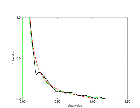
Figure 1: Density of eigenvalues of a Euclidean Random Matrix in three dimensions, density $\rho=1$. The function $f$ is $f(x)=(2\pi)^{-3/2}\exp(-x^{2}/2)$, and the matrix is defined from eq.(48). The full line is the result of a numerical simulation with $N=800$ points, averaged over $100$ samples. The dashed line is the result from the high density expansion. The dash-dotted line is the result from the Gaussian variational approximation (RPA) to the field theory.

We have studied numerically the problem in dimension $d=3$ with the Gaussian function $f(x)=(2\pi)^{-3/2}\exp(-x^{2}/2)$. In this Gaussian case the high density approximation gives a spectrum

$$g(\lambda)\sim{1\over\rho\pi^{2}}{1\over\lambda}\left({1\over 2}\log{\rho\over\lambda}\right)^{1/2}\theta(\rho-\lambda)+C\delta(\lambda)$$ (82)

Notice that this spectrum is supposed to hold away from the small $\lambda$ peak, and in fact it is not normalizable at small $\lambda$.

It is possible to do a variational approximation computation taking care of all the non-linear terms in the action for the fields. This corresponds (as usually) a a resummation of a selected class of diagrams. After some computations, one finds that one needs to solve, given $z=\lambda-i\epsilon$, the following equations for $C(z)\equiv a(z)+ib(z)$:

$$\lambda = \rho{a\over a^{2}+b^{2}}+{1\over 2\pi^{2}}\int_{0}^{\infty}k^{2}dk{e^{k^{2}/2}-u\over\left(e^{k^{2}/2}-a\right)^{2}+b^{2}}$$

$$\epsilon = \rho{b\over a^{2}+b^{2}}-{b\over 2\pi^{2}}\int_{0}^{\infty}k^{2}dk{1\over\left(e^{k^{2}/2}-a\right)^{2}+b^{2}}\ .$$ (83)

One needs to find a solution in the limit where $\epsilon\to 0$.

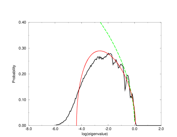
Figure 2: Density of the logarithm (in base 10) of the eigenvalues of a Euclidean Random Matrix in three dimensions, density $\rho=1$ (same data of the previous figure). The dashed line is the result from the high density expansion. The dotted line is the result from the Gaussian variational approximation (RPA) to the field theory.

In fig. (1,2), we plot the obtained spectrum, averaged over 100 realizations, for $N=800$ points at density $\rho=1$ (We checked that with a different number of points the spectrum is similar). Also shown are the high density approximation (82), and the result from the variational approximation. We see from fig.(1) that the part of the spectrum $\lambda\in[0.2,1.5]$ is rather well reproduced from both approximations, although the variational method does a better job at matching the upper edge. On the other hand the probability distribution of the logarithm of the eigenvalues (fig.2) makes it clear that the high density approximation is not valid at small eigenvalues, while the variational approximation gives a sensible result. One drawback of the variational approximation, though, is that it always produces sharp bands with a square root singularity, in contrast to the tails that are seen numerically.

In fig.3, we plot the obtained spectrum, averaged over 200 realizations, for $N=800$ points at density $\rho=0.1$. We show also a low density approximation (that we do not describe here [3]), and the result from the variational approximation. We see from fig.(3) that this value of $\rho=0.1$ is more in the low density regime, and in particular there exists a peak around $\lambda=f(0)$ due to the isolated clusters containing small number of points. The variational approximation gives the main orders of magnitude of the distribution, but it is not able to reproduce the details of the spectrum, in particular the peak due to small clusters. On the other hand the leading term of a low density approximation (introduced in [3]) gives a poor approximation the the overall form of the spectrum. One should use an approach where the advantages of both methods are combined together.

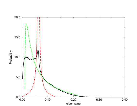
Figure 3: Density of eigenvalues of a Euclidean Random Matrix in three dimensions, density $\rho=0.1$. The function $f$ is $f(x)=(2\pi)^{-3/2}\exp(-x^{2}/2)$, and the matrix is defined from eq.(48) with $u=0$. The full line is the result of a numerical simulation with $N=800$ points, averaged over $200$ samples. The dashed line is the result from a low density expansion introduced in [3]. The dash-dotted line is the result from the Gaussian variational approximation (RPA) to the field theory.

6 Phonons

6.1 Physical Motivations

Inelastic X-ray scattering (IXS) experiments and inelastic neutron scattering on structural glasses and supercooled liquids provided useful information on the dynamics of their amorphous structure, at frequencies larger than $0.1$ THz (see for example [35] and references therein). Those experiments show a regime, when the wavelength of the plane wave is comparable with the inter-particle distance, where the vibrational spectrum can be understood in terms of propagation of quasi-elastic sound waves, the so-called high frequency sound. This high-frequency sound has also been observed in molecular dynamical simulations of strong and fragile liquids, and it displays several rather universal features. In particular, a peak is observed in the dynamical structure factor at a frequency that depends linearly on the exchanged momentum $p$, in the region $0.1p_{0}-1.0p_{0}$, $p_{0}$ being the position of the first maximum in the static structure factor. When extrapolated to zero momentum, this linear dispersion relation yields the macroscopic speed of sound. The width of the spectral line, $\Gamma$ is well fitted by

$$\Gamma(p)=Ap^{x}\quad,\quad x\approx 2\,,$$ (84)

with $A$ displaying a very mild (if any) temperature dependence. Moreover, the same scaling of $\Gamma$ has been found in harmonic Lenhard-Jones glasses [36], and one can safely conclude that the $p^{2}$ broadening of the high-frequency sound is due to small oscillations in the harmonic approximation. In these context other interesting problems related with the high-frequency vibrational excitations of these topologically disordered systems [20] regard the origin of the Boson peak or the importance of localization properties to understand the dynamics of supercooled liquids [38].

The variety of materials where the $p^{2}$ broadening appears suggests a straightforward physical motivation. However, the simplest conceivable approximation, a wave propagating on an elastic medium in the presence of random scatterers, yields Rayleigh dispersion: $\Gamma\propto p^{4}$. This result is very robust: as soon as one assumes the presence of an underlying medium where the sound waves would propagate undisturbed, as in the disordered-solid model [37, 39, 40], the $p^{4}$ scaling appears even if one studies the interaction with the scatterers non-perturbatively [41]. When the distinction between the propagating medium and the scatterers is meaningless (as it happens for topologically disordered systems), the $p^{2}$ scaling is recovered.

We want to investigate the problem from the point of view of statistical mechanics of random matrices, by assuming that vibrations are the only motions allowed in the system. The formalism we shall introduce, however, is not limited to the investigation of the high frequency sound and it could be straightforwardly applied in different physical contexts.

Let us look more carefully at the relation between vibrational dynamics in glasses and random matrices. The dynamical structure factor for a system of $N$ identical particles is defined as:

$$S(p,\omega)=\frac{1}{N}\sum_{i,j}\int dt\ {\mathrm{e}}^{{\mathrm{i}}\omega t}\ \left\langle\,{\mathrm{e}}^{{\mathrm{i}}p\cdot\left(r_{j}(t)-r_{i}(0)\right)}\,\right\rangle\,,$$ (85)

where $\langle\dots\rangle$ denotes the average over the particles positions $r_{j}$ with the canonical ensemble.

Here it is convenient to consider the normal modes of the glass or the supercooled liquid, usually called instantaneous normal modes (INM) because they are supposed to describe the short time dynamics of the particles in the liquid phase [22]. One studies the displacements $u$ around the random positions $x$, by writing the position of the $i$-th particle as ${r}_{i}(t)={x}_{i}+{u}_{i}(t)$, and linearizing the equations of motion. Then one is naturally lead to consider the spectrum of the Hessian matrix of the potential, evaluated on the instantaneous position of the particles. Calling $\omega_{n}^{2}$ the eigenvalues of the Hessian matrix and $e_{n}(i)$ the corresponding eigenvectors, the one excitation approximation to the $S(p,\omega)$ at non zero frequency is given in the classical limit by:

$$S^{(1)}(p,\omega) = \frac{k_{\mathrm{B}}T}{m\omega^{2}}\,\sum_{n=1}^{N}\,Q_{n}(p)\,\delta(\omega-\omega_{n})\,,$$ (86)

$$Q_{n}(p) = |\sum_{i}\,p\cdot e_{n}(i)\exp({\mathrm{i}}p\cdot x_{i})|^{2}\,.$$ (87)

However one cannot always assume that all the normal modes have positive eigenvalues, negative eigenvalues representing the situation where some particles are moving away from the position $x$. Indeed, it has been suggested [38] that diffusion properties in supercooled liquids can be studied considering the localization properties of the normal modes of negative eigenvalues.

A related and better defined problem is the study of normal modes at zero temperature, where the displacements $u$ are taken around the rest positions. By assuming that this structure corresponds to one minimum of the potential energy, one can introduce a harmonic approximation where only the vibrations around these minima are considered, and all the dynamical information is encoded in the spectral properties of the Hessian matrix on the rest positions. The Hessian is in a first approximation a random matrix if these rest positions correspond to a glass phase. It has been shown using molecular dynamics simulation that below the experimental glass transition temperature the thermodynamical properties of typical strong glasses are in a good agreement with such an assumption.

Therefore, the problem of the high-frequency dynamics of the system can be reduced, in its simplest version, to the consideration of random Euclidean matrices, where the entries are deterministic functions (the derivatives of the potential) of the random positions of the particles. As far as the system has momentum conservation in our case, due to translational invariance, all the realizations of the random matrix have a three common normal mode with zero eigenvalue: the uniform translation of the system.

An Euclidean matrix is determined by the particular deterministic function that we are considering, and by the probabilistic distribution function of the particles, that in the INM case is given by the Boltzmann factor. However, for the sake of simplicity we shall concentrate here on the simplest kind of euclidean matrices without spatial correlations and we will neglect the vector indices of the displacement. We consider $N$ particles placed at positions $x_{i},i=1,2,...,N$ inside a box, where periodic boundary conditions are applied. Then, the scalar euclidean matrices are given by eq.(2), where $f(x)$ is a scalar function depending on the distance between pairs of particles, and the positions $\{{x}\}$ of the particles are drawn with a flat probability distribution. Notice that the matrix (2) preserves translation invariance, since the uniform vector $e_{0}(i)=const$ is an eigenvector of $M$ with zero eigenvalue. Since there are not internal indices (the particle displacements are restricted to be all collinear), we cannot separate longitudinal and transversal excitations.

The dynamical structure factor for a scalar Euclidean matrix is given by

$$S_{E}(p,E) = \overline{\sum_{n}Q_{n}(p)\delta(E-E_{n})}\,,$$ (88)

$$Q_{n}(p) = \frac{1}{N}\left|\sum_{i=1}^{N}\,e_{n}(i)\exp({\mathrm{i}}p\cdot x_{i})\right|^{2}\,,$$ (89)

$$S(p,\omega) = 2\omega S_{E}(p,\omega^{2})\,,$$ (90)

where the overline stands for the average over the particles position and we have given the definition either in the eigenvalue space ($S_{E}(p,E)$) and in the frequency space ($S(p,\omega)$).

6.2 A more complex field theory representation

The basic field theory representation is similar to the one of the previous section. The main complication is due to the presence of a diagonal term in the matrix $M$. One way out is to introduce one more pair of Bosonic fields. To perform the spatial integrations it turns out to be convenient to represent the Bosonic fields $\phi$ using new Bosonic fields , i.e.:

$$\chi(x) \equiv \sum_{i,a}(\phi^{(a)}_{i})^{2}\delta(x-x_{i})$$ (91)

$$\psi^{(a)}(x) \equiv \sum_{i}\phi^{(a)}_{i}\delta(x-x_{i})\ ,$$ (92)

and using the “Lagrange multipliers” $\,\hat{\psi^{(a)}}(x),\hat{\chi}(x)$, to enforce the three constraints (92). At this point, the Gaussian variables $\phi^{(a)}_{i}$ are decoupled and can be integrated out.

Skipping intermediate steps and using the fact that all the replicas are equivalent one can write the Green function as a correlation function:

$$G(p,z)=$$

$$\lim_{n\to 0}\frac{1}{N}\int d^{d}xd^{d}y\>\>e^{ip(x-y)}\int{D[\psi^{(a)},\hat{\psi^{(a)}},\chi,\hat{\chi}]\>\psi^{(1)}(x)\psi^{(1)}(y)A^{N}\>\exp({S_{0}})}\ ,$$ (93)

where we have introduced the following quantities:

$$S_{0}\equiv i\sum_{a=1,n}\int d^{d}x\>\hat{\psi}^{(a)}(x)\psi^{(a)}(x)+\int d^{d}x\chi(x)\hat{\chi}(x)$$

$$-\frac{1}{2}\sum_{a=1,n}\int d^{d}xd^{d}y\psi^{(a)}(x)f(x-y)\psi^{(a)}(y)$$

$$A\equiv\int{{d^{d}x}\exp\Phi(x)}$$

$$\Phi(x)\equiv+i\int d^{d}yf(y-x)\chi(y)-\frac{1}{2}\frac{\sum_{a=1,n}{\left(\hat{\psi}^{(a)}(x)\right)}^{2}}{z+\hat{\chi}(x)}\ .$$ (94)

In order to take easily the limits $N,V\to\infty$ in (93) we shall resort to a grand canonical formulation of the disorder, introducing the partition function ${\cal Z}[\rho]\equiv\sum_{N}A^{N}\rho^{N}/N!\>\exp{S_{0}}$. Since the average number of particles $\overline{N}=V\rho\langle A\rangle$, in the $n\to 0$ limit we have that $\langle A\rangle=1$ and the ’activity’ $\rho$ is just the density of points, as before. Furthermore, the Gaussian integration over the fields $\psi^{(a)}$ is easily performed, leading to the field theory:

$${\cal Z}\left[\rho,z\right]=\int{D[\hat{\psi^{(a)}},\chi,\hat{\chi}]\exp{(S^{\prime}_{0}+S_{1})}}\ ,$$ (95)

where

$$S^{\prime}_{0}\equiv-\frac{n}{2}\mbox{Tr}\ln f+\int d^{d}x\chi(x)\hat{\chi}(x)-//\frac{1}{2}\sum_{a=1,n}\int d^{d}xd^{d}y\>\hat{\psi}^{(a)}(x)f^{(-1)}(x-y)\hat{\psi}^{(a)}(y)$$

$$S_{1}\equiv\rho\int d^{d}x\>\left(\exp{\Phi(x)}\right)$$

The resolvent is related to the correlation function by eq.(59). Before computing (59), let us turn to the symmetry due to the translational invariance. Since $e_{n}(i)=constant$ is an eigenvector of zero eigenvalue of the matrix (2) for every disorder realization, we see that Eq.(15) implies:

$$G(p=0,z)=\frac{1}{z}\ .$$ (96)

Interestingly enough, in the framework of the field theory introduced above, that constraint is automatically satisfied, due to the Ward identity linked to that symmetry. The interaction term $\Phi(x)$ is indeed invariant under the following infinitesimal transformation of order $\eta$:

$$\delta\hat{\psi}^{(1)}(x)=i\eta\left(z+\hat{\chi}(x)\right)\,,$$ (97)

$$\delta\chi(x)=2i\eta\int d^{d}yf^{-1}(x-y)\hat{\psi}^{(1)}(y)\left(z+\hat{\chi}(x)\right)\,,$$ (98)

while the whole variation of the action $S=S^{\prime}_{0}+S_{1}$ is due to the non-interacting part $S^{\prime}_{0}$:

$$\delta S=-i\eta\frac{z}{\tilde{f}(0)}\int d^{d}x\hat{\psi}^{(1)}(x)$$ (99)

The invariance of $S_{1}$ hence leads to the following Ward identity:

$$\langle z+\hat{\chi}(x)\rangle=\frac{z}{\tilde{f}(0)}\langle\hat{\psi}^{(1)}(x)\int d^{d}y\>\hat{\psi}^{(1)}(y)\rangle$$ (100)

That is enough to prove that

$$\int d^{d}y\hat{\psi}^{(1)}(0)\hat{\psi}^{(1)}(y)$$ (101)

diverges as $1/z$ at small zeta. If we combine the previous result with the exact relation $\langle\hat{\chi}(x)\rangle=-\rho\tilde{f}(0)$, that can be derived with a different argument, to obtain:

$$(z-\rho\tilde{f}(0))\frac{\tilde{f}(0)}{z}=\int d^{d}y\>\langle\hat{\psi}^{(1)}(x)\hat{\psi}^{(1)}(y)\rangle\ `$$ (102)

that, together with (59), implies the expected constraint $G(p=0,z)=1/z$.

The interacting term in (6.2) is complicated by the presence of an exponential interaction, meaning an infinite number of vertices. In order to perform the explicit computation of the resolvent $G(p,z)$ one has to introduce some scheme of approximation. We have chosen to deal with the high density limit, where many particles lie inside the range of the interaction $f(r)$. The high density limit ($\rho\gg 1$) of (59) is the typical situation one finds in many interesting physical situations, for example the glassy phase. In order to extract the leading term let us make the expansion $\exp\Phi(x)-1\sim\Phi(x)$. In that case the integration over the fields $\chi,\hat{\chi}$ is trivial, because of:

$$\int D[\chi]\exp\left(\int d^{d}x\chi(x)\left[\rho\int d^{d}yf(x-y)+\hat{\chi}(x)\right]\right)=$$

$$\prod_{x}\delta(\hat{\chi}(x)+\rho\tilde{f}(0))$$ (103)

and the fields $\hat{\psi}^{(a)}$ are free. In fact, introducing the quantity $a\equiv z-\rho\tilde{f}(0)$, one remains with the Gaussian integration:

$${\cal Z}\propto\int D[\hat{\psi}^{(a)}]\exp{-\frac{1}{2}\int d^{d}xd^{d}y\sum_{a}\hat{\psi}^{(a)}(x)K^{-1}(x-y)\hat{\psi}^{(a)}(y)}\ ,$$ (104)

where the free propagator $K$ is defined by:

$$K^{-1}(x-y)\equiv f^{-1}(x-y)+\frac{\rho}{a}\delta(x-y)\ .$$ (105)

It is then easy from (59) and (104) to obtain the result:

$$G_{0}(p,z)=\frac{1}{z-\epsilon(p)}\,,$$ (106)

where

$$\epsilon(p)=\sqrt{\rho(\tilde{f}(p)-\tilde{f}(0)}$$ (107)

We see that at the leading order, a plane wave with momentum $p$ is actually an eigenstate of the matrix $M$ with eigenvalue $E$, and the disorder does not play any relevant role. In other words, inside a wavelength $2\pi/p$ there is always an infinite number of particles, ruling out the density fluctuations of the particles: the system reacts as an elastic medium.

Let us finally obtain the density of states at this level of accuracy, using Eq(18) and $G_{0}$:

$$g_{E}(E)=\delta\left(E-\rho\tilde{f}(0)\right)\,.$$ (108)

We obtain a single delta function at $\rho\tilde{f}(0)$, that is somehow contradictory with our result for the dynamical structure factor: from the density of states one would say that the dispersion relation is Einstein’s like, without any momentum dependence! The way out of this contradiction is of course that in the limit of infinite $\rho$ both $\epsilon(p)$ and $\rho\tilde{f}(0)$ diverge. The delta function in eq. (108) is the leading term in $\rho$, while the states that contribute to the dynamical structure factor appear only in the subleading terms in the density of states. The same phenomenon is present in the simpler case discussed in the previous section.

subsectionOne loop

We have seen above that, with the expansion of $\exp\Phi(x)$ up to first order in $\Phi(x)$ the fields $\hat{\psi}$ are non interacting and no self energy is present. Now we shall see that the one-loop correction to that leading term provides the $\frac{1}{\rho}$ contribution to the self energy. In fact by adding the quadratic term to $S_{1}$ the total action becomes (in the $n\to 0$ limit):

$$S=S^{\prime}_{0}+S_{1}\sim S^{\prime}_{0}+\rho\int d^{d}x\>\left(\Phi(x)+\frac{1}{2}\Phi^{2}(x)\right)$$

$$=-\frac{\rho}{2}\int d^{d}xd^{d}y\>\chi(x)f^{(2)}(x-y)\chi(y)+i\int d^{d}x\>b(x)\chi(x)$$

$$--\frac{1}{2}\sum_{a=1,n}\int d^{d}xd^{d}y\>\hat{\psi}^{(a)}(x)c(x-y)\hat{\psi}^{(a)}(y)$$

$$+\frac{\rho}{8}\int d^{d}x\>\left(\frac{\sum_{a=1,n}{\left(\hat{\psi}^{(a)}(x)\right)}^{2}}{z+\hat{\chi}(x)}\right)^{2}\ ,$$ (109)

where

$$b(x) \equiv \hat{\chi}(x)+\rho\tilde{f}(0)-\frac{\rho}{2}\int d^{d}y\>\frac{\sum_{a=1,n}{\left(\hat{\psi}^{(a)}(x)\right)}^{2}}{z+\hat{\chi}(x)}f(y-x)$$

$$c(x-y) \equiv f^{(-1)}(x-y)+\frac{\rho}{z+\hat{\chi}(x)}\delta(x-y)$$ (110)

After doing some computations and adding the two contributions coming two different diagrams one gets

$$G(p,z)=$$

$$G_{0}(p,z)+G_{0}^{2}(p,z)\frac{1}{\rho}\int\frac{d^{d}q}{(2\pi)^{d}}\>G_{0}(q,z)\left(\left[\rho\tilde{f}(p-\emph{q})-\rho\tilde{f}(\emph{q})\right]\right)^{2}$$ (111)

The Dyson resummation of all the higher orders terms, that is built by ’decorating’ recursively all the external legs $G_{0}$ with the one loop correction in (111) gives:

$$G(p,z)=\frac{1}{z-\epsilon(p)-\Sigma_{1}(p,z)}\ ,$$ (112)

where the self-energy $\Sigma_{1}(p,z)$ is given by

$$\Sigma_{1}(p,z)\equiv\frac{1}{\rho}\int\frac{d^{d}q}{(2\pi)^{d}}\>G_{0}(q,z)\left[\rho\tilde{f}(p-\emph{q})-\rho\tilde{f}(\emph{q})\right]^{2}\ .$$ (113)

Let us study in details the low exchanged momentum limit of Eq.(113). It is clear that at $p=0$ the self-energy vanishes, as required by the Ward identity (100). We need to expand $\tilde{f}(p-q)$ for small $p$, that due to the spherical symmetry of $\tilde{f}$ yields

$$\tilde{f}(p-q) = \tilde{f}(q)-(p\cdot q)\,\frac{\tilde{f}^{\prime}(q)}{q}+{\cal O}(p^{2})\,,$$ (114)

$$= \tilde{f}(q)+(p\cdot q)\,\frac{\epsilon^{\prime}(q)}{q\rho}+{\cal O}(p^{2})\,.$$ (115)

Substituting (115) in (113), and performing explicitly the trivial angular integrations in dimensions $d$ we obtain

$$\Sigma_{1}(p,z)\approx p^{2}\frac{2^{1-d}}{\rho d\pi^{d/2}\Gamma(d/2)}\int_{0}^{\infty}dq\,q^{d-1}\frac{\left[\epsilon^{\prime}(q)\right]^{2}}{z-\epsilon(q)}=$$

$$p^{2}\frac{2^{1-d}}{\rho d\pi^{d/2}\Gamma(d/2)}\int_{0}^{\epsilon(q=\infty)}d\epsilon\,\frac{\left[q(\epsilon)\right]^{d-1}}{q^{\prime}(\epsilon)(z-\epsilon)}\,.$$ (116)

In the last equation, we have denoted with $q(\epsilon)$ the inverse of the function $\epsilon(q)$. Setting now $z=E+{\mathrm{i}}0^{+}$, and observing that $\epsilon(p)\approx Ap^{2}$ for small $p$, we readily obtain

$$Re\Sigma_{1}(p,E+{\mathrm{i}}0^{+}) \approx p^{2}\frac{2^{1-d}}{\rho d\pi^{d/2}\Gamma(d/2)}\int_{0}^{\epsilon(q=\infty)}d\epsilon\,\frac{\left[q(\epsilon)\right]^{d-1}}{q^{\prime}(\epsilon)(E-\epsilon)}\,,$$ (117)

$$Im\Sigma_{1}(p,E+{\mathrm{i}}0^{+}) \approx -\frac{\pi 2^{2-d}A}{\rho d\pi^{d/2}\Gamma(d/2)}p^{2}[q(E)]^{d}\,.$$ (118)

Since the principal part is a number of order one, the real part of the self-energy scales like $p^{2}$ (possibly with logarithmic corrections), and thus the speed of sound of the system renormalizes due to the $1/\rho$ corrections. As a consequence, the function $q(E)$ is proportional to $E^{1/2}\sim p$ at the maximum of the function of $p$ $S_{E}(p,E)$, and the width of the peak of the $S_{E}(p,E)$ will scale like $p^{d+2}$. It is then easy to check (see (90)) that in frequency space the width of the spectral line will scale like

$$\Gamma\propto p^{d+1}\,,$$ (119)

as one would expect from Rayleigh scattering considerations.

The result (119) for the asymptotic regime $p<<1$ has been found at the one loop level. In order to predict correctly the spectral properties at very low external momentum $p$, it turns out that one must study the behavior of the two loop contribution, that can be done in details. Nevertheless, the one loop result is already a good starting point to perform detailed comparisons with the numerical simulations. The disadvantage of this approach is that it works near band edge ($\omega=0$ at high $\rho$ but is not suited for producing the whole spectrum. Due to the complication of the action it is not clear how to do a variational computation and the best it can be done at the present moment is a CPA-like approximation described in the next section.

6.3 A CPA like approximation

As in the previous section we consider the resolvent $G(p,z)$ Our aim is to compute $G$ using the appropriate self-consistent equations. A partial resummation of the expansion for the resolvent can be written as

$$G(p,z)=\frac{1}{z-\lambda(p)-\Sigma(p,z)}\,.$$ (120)

The self-energy $\Sigma(p,z)$ is then expanded in powers of $1/\rho$ [3, 8] in the relevant region where $\rho=O(z)$.

Figure 4: The diagrams of the $1/\rho$ expansion that are taken into account in our approach. The numbers correspond to the particle-label repetitions

If we reformulate the $1/\rho$ expansion in a diagrammatic way we can identify those diagrams with the simple topology of Fig. 4. Topologically, these diagrams are exactly those considered in the usual lattice CPA and in other self consistent approximations. The sum of this infinite subset is given by the solution of the integral equation:

$$\Sigma(p,z)=\frac{1}{\rho}\int\!\!\frac{d^{3}q}{(2\pi)^{3}}\left[\rho\left(\hat{f}(\mbox{\boldmath$q$})-\hat{f}(\mbox{\boldmath$p$}-\mbox{\boldmath$q$})\right)\right]^{2}G(p,z),$$ (121)

where the resolvent is given by Eq. (120). The solution gives us the resolvent, and hence the dynamical structure function and density of states (Eq. 122 below).

We are interested to study the solution of Eq. (121) for different values of $z$ and $\rho$. To be definite, we consider an explicit case where the function $f(r)$ has a simple form, namely $f(r)=\exp[-r^{2}/(2\sigma^{2})]$. This is a reasonable first approximation for the effective interaction [9]. We shall take $\sigma$ as the unit of length and set $p_{0}=1/\sigma$, that is a reasonable choice for $p_{0}$ for this Gaussian $f(r)$, as discussed in [9]. In this particular case we will solve numerically the self-consistence equation. We will also evaluate by simulation (using the method of moments [42]) the exact dynamical structure function and the density of states by computing the resolvent for concrete realizations of the dynamical matrix, considering a sufficiently high number of particles so that finite volume effects can be neglected. These numerical results will be supplemented by analytic results, that are $f$-independent and can be obtained in the limits $p\to\infty$ and $p\to 0$.

The infinite momentum limit is particularly interesting because of the remarkable result [7, 8] that the density of states $g(\omega)$ can be written as

$$g(\omega)=\lim_{p\to\infty}\frac{\omega^{2}S^{(1)}(p,\omega)}{k_{\mathrm{B}}Tp^{2}}.$$ (122)

Figure 5: Top: dynamic structure factor as obtained from Eq.(121) (full line) and from simulations [8] (dashes). Bottom: the density of states divided by $\omega^{2}$ (Debye behavior) as obtained from Eq.(123) (full line), simulations (dashes), and first order in the $1/\rho$ expansion (dots).

We easily find that in this limit Eq. (121) can be written as:

$$\frac{1}{\rho{\cal G}(z)}=\frac{z}{\rho}-\hat{f}(0)-{\cal A}{\cal G}(z)-\int\!\!\!\frac{d^{3}q}{(2\pi)^{3}}\hat{f}^{2}(\mbox{\boldmath$q$})G(\mbox{\boldmath$q$},z)\ ,$$ (123)

where

$${\cal G}(z)=\lim_{p\to\infty}G(p,z)$$ (124)

and

$${\cal A}=(2\pi)^{-3}\int\!\!\hat{f}^{2}(\mbox{\boldmath$q$})\,d^{3}q\ .$$ (125)

A simple approximation consists in neglecting the last term in the r.h.s. of (123), that is reasonable at large $z$. This approximation implies a the density of states that is semicircular as a function of $\omega^{2}$, with width proportional to $\sqrt{\rho}$ and centered at $\omega^{2}=\rho\hat{f}(0)$. Translational invariance also requires low-frequency modes. These are given by the neglected term, and in fact it is easy to show that at high density it produces a Debye spectrum that extends between zero frequency and the semicircular part.

In the limit $p\to 0$, the leading contribution to $\Sigma^{\prime\prime}$ comes from $q\gg p$ in Eq. (121), where $G(q,z)\approx{\cal G}(z)$, so we can write for the peak width $\Gamma(p)\approx\Gamma_{0}(p)$, where

$$\Gamma_{0}(p)\equiv\pi\rho\frac{g(\omega_{p})}{2\omega_{p}^{2}}\int\!\!\!\frac{d^{3}q}{(2\pi)^{3}}\left[\hat{f}(\mbox{\boldmath$q$})-\hat{f}(\mbox{\boldmath$p$}-\mbox{\boldmath$q$})\right]^{2}.$$ (126)

The integral is of order $p^{2}$, so if the spectrum is Debye-like for small frequencies, we get $\Gamma(p)\sim p^{2}$.

These considerations are verified by the numerical solution of the Gaussian case, that are shown in Fig. 5 for $\rho=1.0\,\sigma^{-3}$ together with the results for the simulations [8]. Note the good agreement, to be expected for high-densities, and how, for large $p$, $S^{(1)}(p,\omega)$ (Fig. 5, top) tends to the density of states. The density of states from the self-consistent equation (Fig. 5,bottom) also agrees very well with the results from simulations, and is a big improvement over the first term of the expansion in powers of $\rho^{-1}$. The two contributions (Debye and semicircle) mentioned above can be clearly identified. As expected our approximation fails in reproducing the exponential decay of the density of states at high frequencies, that is non perturbative in $1/\rho$ [6] and corresponds to localized states.

Figure 6: Peak width vs. $p$, for $\rho=0.6\sigma^{-3}$. The inset shows that $\Gamma_{0}(p)$ is the dominant contribution at small $p$.

Next in Fig. 6 we plot the linewidth as a function of $p$ as obtained from Eq.(121). Notice that we recover the behavior predicted from the first two non-trivial terms in the expansion in powers of $\rho^{-1}$ [8]: the linewidth is proportional to $p^{2}$ at small $p$ (also predicted by the argument above), then there is a faster growth and finally it approaches to a constant as $S^{(1)}(q,\omega)$ starts to collapse onto the density of states. The inset shows that the contribution Eq. (126) is indeed dominant at small $p$. However, accurate $p^{2}$ scaling is found only for very small momenta ($p/p_{0}<0.1$), while experiments are done at $0.1<p/p_{0}<1$. In this crossover region, our approach predicts the existence of non-universal, model dependent small deviations from $p^{2}$, that are probably hard to measure experimentally. In any case, the effective exponent is certainly less than 4, in contrast with lattice models and consistent with experimental findings. Similar conclusions can be drawn from mode coupling theory (see fig. 8 of [44]).

6.4 The disappearance of phonons

New phenomena are present the function $f$ is no more positive or in the vectorial case. In these case it is possible that the spectrum arrives up to negative values and the density of states $g_{E}$ does not vanish at $E=0$. In principle for a given model we should not expect a sharp transition from the situation where the Debye spectrum holds and $g_{E}(E)\propto E^{1/2}$ because tails are always present. However often tails are small and one can effectively observe a transition from the two regimes.

In the framework where the density of states is computed from a simple integral equation, the tails are neglected and we are in the best situation to observe such a phenomenon.

Let us call $\tau$ a parameter that separate the two regimes. A detailed analysis show that a $\tau=0$ the density of states behaves as

$$g_{E}(E)\propto E^{1/4},$$ (127)

while at small $\tau$ and $E$ we have

$$g_{e}(E,\tau)=E^{1/4}h(\tau E^{1/2}).$$ (128)

The detailed argument is a delicate but let us consider an heuristic version of it.

With some work it is possible to obtain from (121) an integral equation even for the density of states. As a matter of fact, defining ${\cal G}(z)=G(p=\infty,z)$, the density of states turns out to be

$$g_{E}(E)=-{2\over\pi}\,\mathrm{Im}\,{\cal G}(E+i0^{+}).$$ (129)

$\cal G$ being the solution of the following equation:

$$\frac{1}{\rho{\cal G}(z)}=\frac{z}{\rho}-\hat{f}(0)-A{\cal G}(z)-B(z)$$ (130)

where

$$A=(2\pi)^{-3}\int\!\!\hat{f}^{2}(\mbox{\boldmath$q$})\,d^{3}q\ ,$$

$$B(z)=\int\!\!\!\frac{d^{3}q}{(2\pi)^{3}}\hat{f}^{2}(\mbox{\boldmath$q$})G(\mbox{\boldmath$q$},z)\ ,$$ (131)

With this equation, one needs to know the resolvent at all $q$ to obtain the density of states, due to the last term in the r.h.s. This can be done by solving numerically the self-consistent equation of ref. [12], but here we perform an approximate analysis, that is more illuminating.

The solution of the previous equation is

$${\cal G}(z)={-\alpha(z)+\sqrt{\alpha(z)^{2}-4A\rho}\over 2A\rho}\ ,$$ (132)

where

$$\alpha(z)=\hat{f}(0)-\frac{z}{\rho}+B(z)$$ (133)

The crudest approximation is to neglect the dependence of $B(z)$ from $z$ (we will also assume that $B$ is a smooth function of the other parameters). In this case Eq. 130 is quadratic in ${\cal G}$, and one easily finds a semicircular density of states. But the semicircular spectrum misses the Debye part, and a better approximation is needed. So we substitute $G$ in the last term of the r.h.s. by the resolvent of the continuum elastic medium $G_{0}(z,p)=(z-E(p))^{-1}$. This is reasonable because the $f^{2}(q)$ factor makes low momenta dominate the integral, and due to translational invariance $G(z,p)\approx G_{0}(z,p)$ in this region [12]. We shall be looking at small $E$, so to a good approximation

$$B(z)=B_{0}+iB_{1}z^{1/2}$$ (134)

We have two limiting cases. depending on the sign of of $\alpha(0)^{2}-4A\rho$.

• When the semicircular part of the density of states does not reach low frequencies, the square root can be Taylor-expanded, and one gets

  $$g_{e}(E)\approx E^{1/2},$$ (135)

  that is precisely Debye’s law.

• In the opposite situation, on the other hand, the semicircle arrives also at negative values of $E$ and $g_{E}(E)$ is different from zero also if $B_{1}$ where zero.

• Exactly at the critical point we get $g_{E}(E)\propto\sqrt{\sqrt{E}}=E^{1/4}$ that is the announced result.

Mathematically, the instability arises when ${\cal G}(0)$ develops an imaginary part. This can only come from the square root in previous equations. Notice that this instability is a kind of phase transition, where the order parameter is $\mathrm{Im}\,{\cal G}(0)$. Doing a detailed computation on finds that this order parameter behaves as $\tau^{\beta}$, with $\beta=1/2$.

Since the behavior of the propagator at high momentua does not strongly affect the dispersion relation [12], we do not expect deviations from a linear dispersion relation. This has been checked either numerically or solving numerically the self-consistency equation given a particular choice for the function $f(r)$ (see the numerical results section below). It can be argued that this kind of phenomenon is responsible of the Boson peak [13], however we cannot discuss this point for lack of space.

sectionCorrelated points

6.5 Various models

When the points are correlated things become more difficult. Already it is difficult to study the statistical properties of correlated points and it is more difficult to study the properties of the matrices that depends on these points. Although some approaches have been developed that allow us to deal with two points correlations [7, 8], it is not evident how to treat the general case where many points correlations are present.

A particular interesting case is when the matrix and the distribution of the points are related. In the best of the possible words there should be extra symmetries that express this relations.

This field is at its infancy, so that I will only describe some general results, without presenting applications, that for the moment do not still exist for the case of Euclidean random matrices.

In the general case we consider an Hamiltonian $H[x]$, such that the stationary equations

$$F_{i}[x]\equiv{\partial H\over\partial x_{i}}=0$$ (136)

have a large number of solutions.

Let us label these solutions with a index $\alpha$. The probability $P[x]$ of a configuration of the points $x$ is assumed to be given by

$$P[x]\propto\sum_{\alpha}w_{\alpha}\delta(x-x^{\alpha})\,,$$

$$w_{\alpha}\equiv D[M^{\alpha}])\exp(-\beta H[x^{\alpha}])\,,$$ (137)

where the matrix $M$ is given by

$$M^{\alpha}_{i,k}={\partial^{2}H\over\partial x_{i}x_{k}}|_{x=x^{\alpha}}\ .$$ (138)

This problem arises for the first time in the framework of spin glasses [45], but its relevance to glasses has been stressed for the first time in [46] The function $F$ may selects the different type of stationary points.

Different interesting possibilities are:

• $D[M]=1$, i.e. all stationary points have the same weight.

• $D[M]=\mbox{sign}({\det[M]})$, i.e. all stationary points have a weight that can be 1 or -1.

• $D[M]=1$ only if all the eigenvalues are positive, otherwise it is zero (i.e. minima are selected)

We are eventually interested to study the properties of the matrix

$$1\over M[x]-z\,,$$ (139)

when the points $x$ are extracted with the previous probability.

6.6 A new supersymmetry

For simplicity I will only restrict myself to the case $z=0$ where some symmetry are present when $D[M]=\mbox{sign}({\det[M]})$.

Indeed it is evident that

$$\int P[x]d[x]A[x]\propto\int d[x]D[M]\exp(-\beta H[x])\det M[x]|\prod_{i}\delta(F_{i}[x])A[x]$$ (140)

The last term simplify to

$$\int d[x]\exp(-\beta H[x])\det M[x]\prod_{i}\delta(F_{i}[x])A[x]\,,$$ (141)

when $D[M]=\mbox{sign}(\det(M))$. For simplicity let us assume that this is the case, without discussing the physical motivations of this choice.

Using usual representations we can write

$$\overline{M^{-1}_{i,k}}=\int d\mu[x,\lambda,\psi,\overline{\psi}]\;\overline{\psi}_{i}\psi_{k}\,,$$ (142)

where $d\mu$ is a normalizes measure proportional to

$$d[x]d[\lambda]d[\psi]d[\overline{\psi}]\exp\left(-\beta H[x]+i\sum_{k}\lambda_{k}F_{k}[x]+\sum_{k,j}M_{j,k}\overline{\psi}_{j}\psi_{k}\right)\ .$$ (143)

Here the $\psi$ are really Fermionic variables (i.e. anticommuting Grassmann variables): they have been introduced for representing the determinant, however they can also be used to compute the matrix elements of the inverse of the matrix $M$.

It was rather unexpected [47, 54] to discover that also for $\beta\neq 0$ the measure $d\mu$ is invariant under a transformation of Fermionic character of BRST type (a supersymmetry in short). (see for example [53, 48]). If $\epsilon$ is an infinitesimal Grassmann parameter, it is straightforward to verify that (143) is invariant under the following transformation,

$$\delta x_{i}=\epsilon\,\psi_{i}\quad\quad\delta\lambda_{i}=-\epsilon\,\beta\,\psi_{i}\quad\quad\delta\bar{\psi}_{i}=-\epsilon\,x_{i}\quad\quad\delta\psi_{i}=0\quad\quad\quad$$ (144)

This symmetry is extremely important and it is crucial to use approximation methods that do not break it [49][51]. This has been stressed in the spin glass case [54] in the context of the Tap equations [55].

6.7 Physical meaning of the supersymmetry

In this section we will follow a reasoning allowing for an intuitive explanation of the physical meaning of the supersymmetry in terms of a particular behavior of the solutions of the stationary equations [56]-[60].

It may be interesting to concentrate the attention on some of the Ward identities that are generated by the supersymmetry. The simplest one is

$$\langle\overline{\psi}_{j}\psi_{k}\rangle=i\langle\lambda_{j}x_{k}\rangle\ .$$ (145)

Apparently the equation is trivially satisfied. Indeed it is convenient to consider a slightly modified theory where we make the substitution

$$F_{j}\to F_{j}-h\ .$$ (146)

The final effect is to add an extra term in the exponential equal to $i\lambda_{j}h$. In other words the r.h.s of equation 145 is

$${\partial\langle x_{k}\rangle_{h}\over\partial h}|_{h=0}$$ (147)

The l.h.s can also be computed and one finds that eq. (145) becomes

$$\sum_{\alpha}w_{\alpha}{\partial\langle x^{\alpha}_{k}\rangle_{h}\over\partial h}|_{h=0}={\partial\sum_{\alpha^{\prime}}w_{\alpha^{\prime}}\langle x^{\alpha^{\prime}}_{k}\rangle\over\partial h}|_{h=0}\ .$$ (148)

If we consider solutions where the $\det(M)\neq 0$ we have that

$${\partial w_{\alpha}\over\partial h}|_{h=0}=0\,,$$ (149)

so that the previous equation seems to be always satisfied.

However the we must be careful if most of solutions have a very small $\det(M)$. In this case if we first sent $N$ to infinity and after we do the derivative with respect to $h$ we can find that the set of solutions in not a continuos functions of $h$. Solutions may bifurcate or disappear for any arbitrary small variation of $h$ and the previous relations are no more valid.

This phenomenon has been studied in the framework of infinite range random matrices, where the function that plays the role of $H$ is the free energy as function of the magnetizations (i.e. the TAP free energy) in spin glass type models. One finds that depending on the parameters there are two phase, one where the supersymmetry is exact, the other where the supersymmetry is spontaneously broken. This last phenomenon has been discovered last year and at the present moment one is trying to fully understand its consequences.

In the framework of Euclidean random theory there are two questions that are quite relevant and may be the most interesting for Euclidean Random theory:

• How to construct and to use in a practical way a formalism where the supersymmetry of the problem plays a crucial role?

• How to find out if there is a phase where supersymmetry is spontaneously broken and which are the physical effects of such a breaking.

It is quite likely the response to these questions would be very important.

References

- [1]
- [2] T. M. Wun and R. F. Loring, J. Chem. Phys 97, 8368 (1992); Y. Wan and R. Stratt, J. Chem. Phys 100, 5123 (1994); A. Cavagna et al., Phys. Rev. Lett. 83, 108 (1999); G. Biroli, R. Monasson, J. Phys. A: Math. Gen. 32, L255 (1999).
- [3] M. Mézard, G. Parisi, and A. Zee, Nucl. Phys. B559, 689 (1999),
- [4] M. Mézard and G.Parisi, Phys. Rev. Lett. 82 (1999)747.
- [5] B.Coluzzi, G.Parisi and P.Verrocchio, J. Chem. Phys. 112, 2933 (2000), B.Coluzzi, G.Parisi and P. Verrocchio, Phys. Rev. Lett. 84,306 (2000)
- [6] A. Zee and I. Affleck, J. Phys: Condens. Matter 12, 8863 (2000).
- [7] V. Martín-Mayor, M. Mézard, G. Parisi, and P. Verrocchio, “The dynamical structure factor in topologically disordered systems” cond-mat 0008472v1 (unpublished).
- [8] V. Martín-Mayor, M. Mézard, G. Parisi, and P. Verrocchio, J. Chem. Phys. 114, 8068 (2001).
- [9] T. S. Grigera et al., cond-mat/0104433 (to be published in Philos. Mag. B).
- [10] T. S. Grigera et al., to be published.
- [11] T.S. Grigera, V. Martín-Mayor, G. Parisi and P. Verrocchio, preprint cond-mat/0110129.
- [12] T.S. Grigera, V. Martín-Mayor, G. Parisi and P. Verrocchio, Phys. Rev. Lett. 87 085502 (2001)
- [13] T.S. Grigera, V. Martín-Mayor, G. Parisi and P. Verrocchio, Phys. Rev. Lett. 87 085502 (2001), T.S. Grigera, V. Martín-Mayor, G. Parisi and P. Verrocchio, cond-mat/0104433 and cond-mat/0301103 (to be published on Nature).
- [14] A. Cavagna, I. Giardina, G. Parisi, J. Phys. A 30 (1997) 7021.
- [15] Cavagna A, Giardina I and Parisi G 1998 Phys. Rev. B 57 11251. i
- [16] S. Ciliberti, T.S. Grigera, V. Martín-Mayor, G. Parisi and P. Verrocchio,
- [17] See Efetof’s lectures at thi
- [18] W. Götze and L. Sjogren, , Rep. Prog. Phys. 55 241 (1992); W. Kob and H. C. Andersen, Phys. Rev. Lett. 73, 1376 (1994).
- [19] G. Parisi J. Phys A 114 (1981) 735, An Introduction to the Statistical Mechanics of Amorphous Systems, in Recent Advances in Field Theory and Statistical Mechanics, edited by J.-B. Zuber and R. Stora (North-Holland, Amsterdam, Netherlands, 1984).
- [20] See S.R. Elliot Physics of amorphous materials, Longman (England 1983).
- [21] See e.g. J. M. Ziman, Models of disorder, Cambridge University Press, Cambdrige (1979).
- [22] T. Keyes, J. Phys. Chem. A 101, 2921 (1997).
- [23] A. Cavagna, Europhys. Lett. 53, 490 (2001).
- [24] L. Angelani, R. Di Leonardo, G. Ruocco, A. Scala, and F. Sciortino, Phys. Rev. Lett. 85, 5356 (2000), K. Broderix, K. K. Bhattacharya, A. Cavagna, A. Zippelius, and I. Giardina, Phys. Rev. Lett. 85, 5360 (2000), T.S. Grigera, A. Cavagna, I.Giardina and G. Parisi, Phys. Rev. Lett. 88, 055502 (2002).
- [25] G. Parisi On the origine of the Boson peak, cond-mat/0301284, Proceeding of the Pisa conference September 2002, to be published on Journal of Physics; cond-mat/030128 Euclidean random matrices, the glass transition and the Boson peak, proceeding of the Messina conference in honour of Gene Stanley, Physica A in press.
- [26] A.Cavagna, I.Giardina, G.Parisi, Phys. Rev. Lett. 83, 108 (1999)
- [27] G. Parisi and N. Sourlas, Phys. Rev. Lett. 43 (1979) 744; Nucl. Phys. B 206 (1982) 321. J. Cardy, Phys. Lett. 125B (1983) 470. A. Klein and J. Fernando-Perez, Phys.Lett. 125B (1983) 473.
- [28] Parisi G and Sourlas N 1982 Nucl. Phys. B 206, 321.
- [29] A Poliakiov, Soviet Phys. JEPT 50, 353 (1970).
- [30] A.Migdal, (private comunication).
- [31] R. Abou-Chacra, P.W. Anderson, and D.J. Thouless, J. Phys. C 5, 1734 (1973). H. Kunz, J. Physique 44, L411 (1883). E.N. Economou and M.H. Cohen, Phys. Rev. B 5, 2931 (1972). A.D. Mirlin and Y.V. Fyodorov, J. Phys. A: Math. Gen. 24, 2273 (1991). A.D. Mirlin and Y.V. Fyodorov, Nucl. Phys. B 366, 507 (1991).
- [32] P. Cizeau and J.P. Bouchaud, Phys. Rev. E 50, 1810 (1994). G.J. Rodgers and A.J. Bray, Phys. Rev. B 37, 3557 (1988). A.J. Bray and G.J. Rodgers, Phys. Rev. B 38, 11461 (1988). G. Biroli and R. Monasson, e-print cond-mat/9902032 (1999).
- [33] A. Cavagna, I. Giardina and G. Parisi, Phys. Rev. Lett. 83 108 (1999).
- [34] A. Zee, I. Affleck, J. Phys.: Cond. Matter 12, 8863 (2000);
- [35] Pilla, O. et al., Nature of the Short Wavelength Excitations in Vitreous Silica: An X-Ray Brillouin Scattering Study. Phys. Rev. Lett. 85, 2136–2139 (2000).
- [36] G. Ruocco et al., Phys. Rev. Lett. 84, 5788 (2000).
- [37] J. Horbach et al., J. Phys. Chem. B 103, 4104 (1999).
- [38] S.B. Bembenek and S.D. Laird, J. Chem. Phys 104. 5199 (1996)
- [39] W. Schirmacher, G. Diezemann and C. Ganter, Phys. Rev. Lett. 81, 136 (1998)
- [40] M. Montagna et al. Phys. Rev. lett. 83, 3450 (1999).
- [41] V. Martín-Mayor et al., Phys. Rev. E 62, 2373 (2000).
- [42] C.Benoit, E.Royer and G.Poussigue, J. Phys Condens. Matter 4. 3125 (1992), and references therein; C.Benoit, J. Phys Condens. Matter 1. 335 (1989), G.Viliani et al. Phys. Rev. B 52, 3346 (1995). Phys. Rev. E.
- [43] P. Turchi, F. Ducastelle and G. Treglia, J. Phys. C 15, 2891 (1982).
- [44] W. Götze and M. R. Mayr, Phys. Rev. E 61, 587 (2000).
- [45] Mézard M, Parisi G and Virasoro M.A., Spin glass theory and beyond”, World Scientific (1987).
- [46] G. Parisi A pedagogical introduction to the replica method for fragile glasses, cond-mat/9905318, Phil. Mag. in press.
- [47] Cavagna A, Garrahan J P and Giardina I 1998 J. Phys. A: Math. Gen. 32 711.
- [48] Zinn-Justin J, 1989 Quantum Field Theory and Critical Phenomena, (Clarendon Press, Oxford).
- [49] Kurchan J 1991 J. Phys. A: Math. Gen. 24 4969.
- [50] Kurchan J 2002 Preprint cond-mat/0209399.
- [51] For an illuminating discussion of the problem of removing the determinant in the supersymmetric formalism see [49, 50] and [28].
- [52] A. Bray and M. Moore, e-print cond-mat/0305620.
-
[53]
C. Becchi, A. Stora and R. Rouet, Commun. Math. Phys. 42 (1975) 127.
I.V. Tyutin Lebdev preprint FIAN 39 (1975) unpublished. - [54] A. Cavagna, I. Giardina, G. Parisi and M. Mezard, J. Phys. A 36 (2003) 1175.
- [55] D. J. Thouless, P. W. Anderson and R. G. Palmer, Phil. Mag. 35 (1977) 593.
- [56] A. Crisanti, L. Leuzzi, G. Parisi, T. Rizzo, Phys. Rev. B, 68 (2003) 174401; Phys. Rev. Lett. 92, 127203 (2004), Phys. Rev. B 70, 064423 (2004).
- [57] A. Crisanti, L. Leuzzi, T. Rizzo, Eur. Phys. J. B, 36 (2003) 129-136; Complexity in Mean-Field Spin-Glass Models: Ising -spin, cond-mat/0406649.
- [58] A. Crisanti, L. Leuzzi, Phys. Rev. B 70, 014409 (2004), The spherical spin glass model: an exactly solvable model for glass to spin-glass transition cond-mat/0407129.
- [59] A, Annibale, A. Cavagna, I. Giardina, G. Parisi, Phys. Rev. E 68, 061103 (2003); A, Annibale, A. Cavagna, I. Giardina, G. Parisi, Elisa Trevigne J. Phys. A 36, 10937 (2003); A. Cavagna, I. Giardina, G. Parisi,Phys. Rev. Lett. 92, 120603 (2004); A. Annibale, G. Gualdi, A. Cavagna J. Phys. A: Math. Gen. 37 (2004) 11311, A. Cavagna, I. Giardina, G. Parisi, Phys. Rev. B 71 (2005) 024422.
- [60] G. Parisi, T. Rizzo On Supersymmetry Breaking in the Computation of the Complexity cond-mat/0401509; Zero-Temperature Limit of the SUSY-breaking Complexity in Diluted Spin-Glass Models cond-mat/0411732
- [61] T. Rizzo Tap Complexity, the Cavity Method and Supersymmetry cond-mat/0403261, T. Rizzo On the Complexity of the Bethe Lattice Spin Glass cond-mat/0404729;