Time correlation functions in Vibration-Transit theory of liquid dynamics

Abstract

Within the framework of V-T theory of monatomic liquid dynamics, an exact equation is derived for a general equilibrium time correlation function. The purely vibrational contribution to such a function expresses the system’s motion in one extended harmonic random valley. This contribution is analytically tractable and has no adjustable parameters. While this contribution alone dominates the thermodynamic properties, both vibrations and transits will make important contributions to time correlation functions. By way of example, the V-T formulation of time correlation functions is applied to the dynamic structure factor $S(q,\omega)$. The vibrational contribution alone is shown to be in near perfect agreement with low-temperature molecular dynamics simulations, and a model simulating the transit contribution with three adjustable parameters achieves equally good agreement with molecular dynamics results in the liquid regime. The theory indicates that transits will broaden without shifting the Rayleigh and Brillouin peaks in $S(q,\omega)$, and this behavior is confirmed by the MD calculations. We find the vibrational contribution alone gives the location and much of the width of the liquid-state Brillouin peak. We also discuss this approach to liquid dynamics compared with potential energy landscape formalisms and mode coupling theory, drawing attention to the distinctive features of our approach and to some potential energy landscape results which support our picture of the liquid state.

I Introduction

Long ago, Frenkel Frenkel (1926, 1946) noted that the liquid-solid phase transition has only a small effect on volume, cohesive forces, and specific heat, while the liquid diffuses much more rapidly than the solid. From these facts he argued that the motion of a liquid atom consists of approximately harmonic oscillations about an equilibrium point, while the equilibrium point itself jumps from time to time. Following this picture, Singwi et al. Singwi and Sjölander (1960); Rahman et al. (1961, 1962a, 1962b); Damle et al. (1968) studied a series of models in which a molecule undergoes vibrational motion for a time, then undergoes continuous diffusion for a time. With adjustable parameters, the model was able to account for incoherent parts of the neutron scattering data for water and lead. In discussing the theory of supercooled liquids and the glass transition, Goldstein Goldstein (1969) presented an insightful description of the potential energy landscape, and of the vibrations about local minima and the transitions over barriers. From computer simulations, Stillinger and Weber Stillinger and Weber (1982a, b, 1984) found the local minima and named them “inherent structures”. They suggested that the equilibrium properties of liquids result from vibrational excitations within, and shifting equilibria between, these structures. In the same spirit, Zwanzig Zwanzig (1983) suggested an approximation for the velocity autocorrelation function, in which that function evaluated for the vibrations within a representative potential energy valley is multiplied by a relaxation factor to account for the hops between valleys. Following these ideas, an active research program has developed, which will be summarized in Sec. V.

In developing V-T theory for monatomic liquids, our initial goal was to construct an approximate but reasonably accurate Hamiltonian, from which the partition function can be calculated analytically and without adjustable parameters Wallace (1997a). This is the most basic formulation available to condensed matter theory, and it was not available for liquids prior to V-T theory. In constructing a tractable model for the potential energy surface, the following three new results were established. (1) From extensive and highly accurate analysis of experimental specific heat data for the elemental liquids at melt, the atomic motion was shown to consist almost entirely of vibrations within nearly-harmonic many-atom valleys Wallace (1997a). (2) From highly accurate analysis of experimental entropies of melting of the elements, the disordering entropy was shown to be a universal constant plus small scatter Wallace (1991, 1992, 1997b). (3) From symmetry considerations it was concluded that the noncrystalline valleys belong to two classes Wallace (1997a): (a) symmetric valleys, which have remnant crystalline symmetry and consequently have a broad range of structural potentials and vibrational frequency distributions, and (b) random valleys, which are of overwhelming numerical superiority and which all have the same structural potential and vibrational frequency distribution. This picture of the potential surface has since been verified by computer studies Wallace and Clements (1999); Clements and Wallace (1999). Only the random valleys need to be considered further, since they completely dominate the potential surface. The number of random valleys is fixed by the universal disordering entropy of the elemental liquids Wallace (1997a). Defining an extended random valley to be the harmonic extension to infinity of a random valley, with intervalley intersections ignored, the leading order Hamiltonian is the sum of extended random valley Hamiltonians, the corresponding partition function is called the vibrational partition function, and any statistical mechanical quantity calculated using this Hamiltonian is called its vibrational contribution Wallace (1997a). The vibrational contribution alone gives an accurate account of the thermodynamic properties of the elemental liquids, without adjustable parameters Wallace (1997a, 1998); Chisolm and Wallace (2004). No other theory does this. Beyond the vibrational contribution, corrections for anharmonicity and for the presence of intervalley intersections are well defined and, though complicated, they are small Wallace (1997a).

In V-T theory, the motion of a liquid system across the boundary between two random valleys is a transit. We have argued that, because of the local character of equilibrium fluctuations in a many particle system, each transit is accomplished by a small local group of atoms Wallace (1997a). Further, because of the dominance of the vibrational contribution to thermodynamic functions, the intervalley intersections must be rather sharp, and transits nearly instantaneous Wallace (1997a). These predictions have since been verified by computer simulations Wallace et al. (2001). In equilibrium, transits are crucial in allowing the system to visit all the random valleys and thus exhibit the correct liquid entropy. Transits are the expression in V-T theory of the equilibrium jumps of Frenkel Frenkel (1946, 1926), and of the barrier hops of Goldstein Goldstein (1969) and Stillinger and Weber Stillinger and Weber (1982a, b, 1984).

In practical applications, V-T theory remains accurate when anharmonicity is neglected entirely. Then the motion consists of the vibrational contribution, for which we have exact analytic equations, plus transits over perfectly sharp intervalley intersections, whose effect we have modeled. In this way, a one-parameter model accounts for the temperature dependence of the specific heat of liquids, as exemplified by the experimental data for mercury Wallace (1998). For a model system, equations were written for the liquid free energy, the glass free energy, and for the nonequilibrium rate processes which occur in the liquid-glass transition region where the free energy is not defined Wallace (1999). This model qualitatively reproduces the results of massive rate-dependent MD calculations of Vollmayr, Kob, and Binder Vollmayr et al. (1996). A one-parameter model for the velocity autocorrelation function gives a good account of MD calculations for temperatures from zero to $3T_{m}$ Chisolm et al. (2001). Hence we have verified the applicability of the equations of V-T theory for the glass, for the glass-transition region, and for the liquid to very high temperatures. A review of V-T theory and its applications, and relations to other theoretical developments, has been presented Chisolm and Wallace (2001).

By now we have learned enough about V-T theory to undertake an exact formulation of time correlation functions. That is the purpose of the present paper. Through linear response theory, time correlation functions contain information on nonequilibrium processes (see Hansen and McDonald (1986), Ch. 7 and 8). Hence in contrast to thermodynamic properties, transits are expected to make a significant contribution to time correlation functions. Though we have previously studied the velocity autocorrelation function Chisolm et al. (2001), here the theory will be illustrated by the density autocorrelation function $F(q,t)$, since this function probes the atomic motion on a more detailed level.

In Sec. II, formally exact statistical mechanical expressions for the partition function, equilibrium statistical averages, and time correlation functions are derived. In Sec. III, we consider the purely vibrational contribution to equilibrium statistical averages (when transits are neglected) and extend the formalism to include time correlation functions. The vibrational contribution to $F(q,t)$, and to its Fourier transform $S(q,\omega)$, are derived in Sec. IV. $S(q,\omega)$ is of interest because it is directly observed in inelastic neutron and x-ray scattering experiments. We then consider a model for incorporating the transit contributions to $F(q,t)$ and $S(q,\omega)$, and we compare the predictions of V-T theory with MD calculations. Our treatment is based on classical statistical mechanics, since this is highly accurate for nearly all the elemental liquids, and is appropriate for comparison with MD. In Sec. V our conclusions, methods, and aims are related to the potential energy landscape and mode coupling theory programs, and we note both significant agreements and divergences. We summarize our results and emphasize the most important conclusions in Sec. VI.

II Statistical averages and time correlation functions

For simplicity we think of an $N$-atom system in a cubic box, with the motion governed by periodic boundary conditions. Atom $K$ at time $t$ has position $\bm{r}_{K}(t)$ and momentum $\bm{p}_{K}(t)$, for $K=1,\dots,N$. The total potential energy is $\Phi(\{\bm{r}_{K}\})$, and the Hamiltonian is

$${\mathcal{H}}=\sum_{K}\frac{\bm{p}_{K}^{2}}{2M}+\Phi(\{\bm{r}_{K}\}).$$ (1)

The set $\{\bm{r}_{K}\}$ represents a point in configuration space. If the potential valleys are denoted by the index $\gamma$, our decomposition of the potential surface means that every accessible configuration is in one and only one valley $\gamma$. For equilibrium statistical mechanical averages, only the random valleys need to be considered.

The canonical partition function $\mathcal{Z}$ is

$${\mathcal{Z}}=\sum_{\gamma}{\mathcal{Z}}_{\gamma},$$ (2)

where $\gamma$ is a random valley, and

$${\mathcal{Z}}_{\gamma}=\frac{1}{h^{3N}}\int d\bm{p}_{1}\dots d\bm{p}_{N}\int_{\gamma}d\bm{r}_{1}\dots d\bm{r}_{N}\;e^{-\beta{\mathcal{H}}}.$$ (3)

The integral $\int_{\gamma}$ is over the domain of valley $\gamma$, where particle permutations are not allowed. The configuration integral is the same in the thermodynamic limit for each random valley, hence we can define the random valley partition function ${\mathcal{Z}}_{rv}$ as ${\mathcal{Z}}_{\gamma}$ for any random valley $\gamma$. We write the number of random valleys as $w^{N}$, where $w$ is a parameter to be determined. Then

$${\mathcal{Z}}=w^{N}{\mathcal{Z}}_{rv}.$$ (4)

This is exact in the thermodynamic limit. The factor $w^{N}$ gives a contribution $Nk\ln w$ to the entropy, and appears in no other thermodynamic function. Calibration to experimental entropy of melting for the elements gives $\ln w=0.80$ Wallace (1997a).

Thermodynamic properties such as energy and pressure are given by equilibrium statistical mechanical averages of the form $\langle A\rangle$, where $A(\{\mathbf{r}_{K},\mathbf{p}_{K}\})$ is a time-independent quantity depending on atomic positions and momenta. With our decomposition of configuration space, the average is

$$\langle A\rangle=\frac{\sum_{\gamma}\int d\bm{p}_{1}\dots d\bm{p}_{N}\int_{\gamma}d\bm{r}_{1}\dots d\bm{r}_{N}\;A\;e^{-\beta{\mathcal{H}}}}{\sum_{\gamma}\int d\bm{p}_{1}\dots d\bm{p}_{N}\int_{\gamma}d\bm{r}_{1}\dots d\bm{r}_{N}\;e^{-\beta{\mathcal{H}}}}.$$ (5)

The denominator is proportional to $\mathcal{Z}$, and just as in Eqs. (2-4), every term in the $\sum_{\gamma}$ in the denominator is equal, and the same is true of the numerator, with the result

$$\langle A\rangle=\langle A\rangle_{rv},$$ (6)

where $\langle\ldots\rangle_{rv}$ is the average over the domain of a single random valley.

We now turn to time correlation functions. Let $B(t)$ be a quantity depending on atomic positions and momenta as they change in time, so that $B(t)=B(\{\mathbf{r}_{K}(t),\mathbf{p}_{K}(t)\})$. For complex $B$, the corresponding autocorrelation function is

$$C(t)=\langle B(t)B^{*}(0)\rangle,$$ (7)

which again invoking the configuration space decomposition becomes

$$C(t)=\frac{\sum_{\gamma}\int d\bm{p}_{1}\dots d\bm{p}_{N}\int_{\gamma}d\bm{r}_{1}\dots d\bm{r}_{N}\;B(t)B^{*}(0)\;e^{-\beta{\mathcal{H}}}}{\sum_{\gamma}\int d\bm{p}_{1}\dots d\bm{p}_{N}\int_{\gamma}d\bm{r}_{1}\dots d\bm{r}_{N}\;e^{-\beta{\mathcal{H}}}},$$ (8)

where the zero-time variables in $B^{*}(0)$ are identical with the integration variables. When $t=0$, this quantity is a fluctuation, and is just a special case of the average considered in the previous paragraph, and so

$$C(0)=\langle B(0)B^{*}(0)\rangle_{rv}.$$ (9)

When $t\neq 0$, however, this is not true, because the system may be in a different random valley at time $t$ than at time 0, so the variable $B(t)B^{*}(0)$ in Eq. (8) has to be evaluated along the equilibrium trajectory of the system. For this reason the calculation of time correlation functions involves difficulties that are absent when computing thermodynamic quantities.

III Vibrational Contribution to time correlation functions

In evaluating the partition function and corresponding equilibrium thermodynamic functions, we previously developed a tractable model for the vibrational contribution Wallace (1997a). In this model, the intersections among valleys are ignored, each random valley is extended to infinite energy, and averages of the vibrational motion are evaluated for one extended random valley. The model is applied to time correlation functions in the present Section.

For configurations in random valley $\gamma$, it is useful to write the position of atom $K$ as

$$\bm{r}_{K}(t)=\bm{R}_{K}(\gamma)+\bm{u}_{K}(t),$$ (10)

where $\bm{R}_{K}(\gamma)$ is the equilibrium position and $\bm{u}_{K}(t)$ is the displacement from equilibrium. The set $\{\bm{R}_{K}(\gamma)\}$ is the structure $\gamma$. The potential energy in valley $\gamma$ is denoted $\Phi(\gamma)$, and is expanded about equilibrium as

$$\Phi(\gamma)=\Phi_{0}(\gamma)+\Phi_{2}(\gamma)+\Phi_{anh}(\gamma),$$ (11)

where $\Phi_{0}(\gamma)$ is the structure potential, $\Phi_{2}(\gamma)$ is the contribution quadratic in displacements, and $\Phi_{anh}(\gamma)$ is the remainder of $\Phi(\gamma)$, the anharmonic part. The anharmonic contribution is almost always small, often negligible. The complicated part of $\Phi(\gamma)$ is the presence on its boundary of intersections with neighboring valleys. But $\Phi(\gamma)$ is a function in $3N$ dimensions, and in most directions there are no such intersections at energies accessible to the liquid. It is only a few directions where low lying valley-valley intersections are present, and it is only in these few directions where transits occur. Hence to describe the vibrational motion alone, we shall ignore intervalley intersections, and as a leading approximation we shall also neglect anharmonicity. The corresponding extended random valley has potential energy

$$\Phi=\Phi_{0}+\frac{1}{2}\sum_{KLij}\Phi_{Ki,Lj}u_{Ki}u_{Lj},\;\;\;\;\;\;\;0\leq u_{Ki}<\infty.$$ (12)

The notation is $i$, $j=$ Cartesian component $x,y,z$, and $\Phi_{Ki,Lj}$ are second position derivatives of $\Phi$ at equilibrium. The index $\gamma$ is suppressed in Eq. (12).

The Hamiltonian for motion in an extended random valley is denoted ${\mathcal{H}}_{vib}$, for vibrations, and is

$${\mathcal{H}}_{vib}=\Phi_{0}+\sum_{Ki}\frac{p_{Ki}^{2}}{2M}+\frac{1}{2}\sum_{KLij}\Phi_{Ki,Lj}u_{Ki}u_{Lj}.$$ (13)

It is useful to transform from displacements to normal modes of vibration. The normal modes are labeled $\lambda=1,\dots,3N$, their coordinates are $Q_{\lambda}$, and the transformation of displacements is

$$u_{Ki}(t)=\sum_{\lambda}w_{Ki,\lambda}\;Q_{\lambda}(t),$$ (14)

where for each $\lambda$, $w_{Ki,\lambda}$ are $3N$ real components of eigenvector $\lambda$. The eigenvectors diagonalize the matrix of potential energy coefficients $\Phi_{Ki,Lj}$, and they satisfy

$$\sum_{Ki}w_{Ki,\lambda}w_{Ki,\lambda^{\prime}}=\delta_{\lambda\lambda^{\prime}},\;\;\;\mbox{orthonormality;}$$ (15)

$$\sum_{\lambda}w_{Ki,\lambda}w_{Lj,\lambda}=\delta_{KL}\delta_{ij},\;\;\;\mbox{completeness.}$$ (16)

For a given extended random valley, its microscopic geometry is encoded in its eigenvectors and its structure. The Hamiltonian (13) transforms to

$${\mathcal{H}}_{vib}=\Phi_{0}+\sum_{\lambda}\left[\frac{P_{\lambda}^{2}}{2M}+\frac{1}{2}M\omega_{\lambda}^{2}Q_{\lambda}^{2}\right],$$ (17)

where $P_{\lambda}=M\dot{Q}_{\lambda}$, and where $\omega_{\lambda}$ is the vibrational frequency of mode $\lambda$. By definition, $\omega_{\lambda}^{2}>0$ for $3N-3$ modes, and $\omega_{\lambda}^{2}=0$ for the three modes of uniform translation. It is understood that the translational modes are omitted from statistical mechanical analyses. The structural potential $\Phi_{0}$, and the distribution $g(\omega)$ of normal mode frequencies, are each the same for all random valleys of a given material.

The partition function is written in Eq. (4). The vibrational contribution is ${\mathcal{Z}}_{vib}=w^{N}{\mathcal{Z}}_{hrv}$, where ${\mathcal{Z}}_{hrv}$ is the partition function for an extended harmonic random valley. The result is

$${\mathcal{Z}}_{vib}=w^{N}e^{-\beta\Phi_{0}}\prod_{\lambda}\frac{kT}{\hbar\omega_{\lambda}}.$$ (18)

This is subject to a correction for anharmonicity, and a correction to recover the proper domain of integration for ${\mathcal{Z}}_{\gamma}$, or ${\mathcal{Z}}_{rv}$. The latter is called the boundary correction. Comparison with experimental data shows that both corrections are small for elemental liquids at melt.

The time correlation function $C(t)$ is written in Eq. (8). The vibrational contribution is $C_{vib}(t)$, obtained by replacing each random valley by its extension. The system then remains in a single random valley, and Eq. (8) reduces to

$$C_{vib}(t)=\left<B(t)B^{*}(0)\right>_{hrv},$$ (19)

where $\left<\dots\right>_{hrv}$ is the average for an extended harmonic random valley. The average in Eq. (19) can be resolved into normal-mode time correlation functions. In quadratic order these functions are

$$\left<Q_{\lambda}(t)Q_{\lambda^{\prime}}(0)\right>_{hrv}=\frac{kT}{M\omega_{\lambda}^{2}}\delta_{\lambda\lambda^{\prime}}\cos\omega_{\lambda}t,\\$$ (20)

$$\left<P_{\lambda}(t)\;P_{\lambda^{\prime}}(0)\right>_{hrv}=MkT\delta_{\lambda\lambda^{\prime}}\cos\omega_{\lambda}t,\\$$ (21)

$$\left<Q_{\lambda}(t)\;P_{\lambda^{\prime}}(0)\right>_{hrv}=0.$$ (22)

An exemplary time correlation function is studied in the next Section.

IV The Density Autocorrelation Function

The density autocorrelation function, or intermediate scattering function, is $F(q,t)$,

$$F(q,t)=\frac{1}{N}\left<\rho(\bm{q},t)\rho(-\bm{q},0)\right>,$$ (23)

where $\rho(\bm{q},t)$ is the Fourier transform of the density operator,

$$\rho(\bm{q},t)=\sum_{K}e^{-i\bm{q}\cdot\bm{r}_{K}(t)}.$$ (24)

First we want to evaluate the vibrational contribution to $F(q,t)$. From Eq. (19), this is

$$F_{vib}(q,t)=\frac{1}{N}\left<\rho(\bm{q},t)\rho(-\bm{q},0)\right>_{hrv}.$$ (25)

Because an equilibrium liquid is macroscopically isotropic, the average in (23), or in (25), cannot depend on the angle of $\bm{q}$ in the thermodynamic limit. But we need to treat a finite system, for which numerical evaluations are possible. For a finite cubic system with periodic boundary conditions, the $\bm{q}$ form a discrete allowed set of wavevectors consistent with the periodicity. We are therefore allowed to average over the directions of the allowed $\bm{q}$. Then Eq. (25) becomes

$$F_{vib}(q,t)=\frac{1}{N}\left<\left<\rho(\bm{q},t)\rho(-\bm{q},0)\right>_{hrv}\right>_{\bm{q}^{\ast}},$$ (26)

where $\left<\dots\right>_{\bm{q}^{\ast}}$ is the average over the star of $\bm{q}$.

For motion in an extended random valley, $\bm{r}_{K}(t)$ is written from Eq. (10), and the average in Eq. (26) works out as (the algebra is the same as for the crystal Lovesey (1984); Glyde (1994))

$$\left<\rho(\bm{q},t)\rho(-\bm{q},0)\right>_{hrv}$$ (27)

$$=\sum_{KL}e^{-i\bm{q}\cdot\bm{R}_{KL}}\left<e^{-i\bm{q}\cdot(\bm{u}_{K}(t)-\bm{u}_{L}(0))}\right>_{hrv}$$

$$=\sum_{KL}e^{-i\bm{q}\cdot\bm{R}_{KL}}e^{-\frac{1}{2}\left<\left[\bm{q}\cdot(\bm{u}_{K}(t)-\bm{u}_{L}(0))\right]^{2}\right>_{hrv}},$$

where $\bm{R}_{KL}=\bm{R}_{K}-\bm{R}_{L}$. The displacement averages simplify to

$$-\frac{1}{2}\left<\left[\bm{q}\cdot(\bm{u}_{K}(t)-\bm{u}_{L}(0))\right]^{2}\right>_{hrv}=$$ (28)

$$-W_{K}(\bm{q})-W_{L}(\bm{q})+\left<\bm{q}\cdot\bm{u}_{K}(t)\;\bm{q}\cdot\bm{u}_{L}(0)\right>_{hrv}.$$

$W_{K}(\bm{q})$ is the Debye-Waller factor for atom K,

$$W_{K}(\bm{q})=\frac{1}{2}\left<(\bm{q}\cdot\bm{u}_{K})^{2}\right>_{hrv}.$$ (29)

The time dependence is entirely contained in the displacement-displacement correlation functions $\left<\bm{q}\cdot\bm{u}_{K}(t)\;\bm{q}\cdot\bm{u}_{L}(0)\right>_{hrv}$. For a random valley, these functions vanish as $t\rightarrow\infty$. Hence it is convenient to write $F(q,t)$ in the form

$$F_{vib}(q,t)=F_{vib}(q,\infty)+\left[F_{vib}(q,t)-F_{vib}(q,\infty)\right],$$ (30)

where

$$F_{vib}(q,\infty)=\frac{1}{N}\left<\sum_{KL}\cos\bm{q}\cdot\bm{R}_{KL}e^{-W_{K}(\bm{q})}e^{-W_{L}(\bm{q})}\right>_{\bm{q}^{\ast}},$$ (31)

$$F_{vib}(q,t)-F_{vib}(q,\infty)=\frac{1}{N}\Bigg{<}\sum_{KL}\cos\bm{q}\cdot\bm{R}_{KL}$$ (32)

$$\times\;e^{-W_{K}(\bm{q})}e^{-W_{L}(\bm{q})}\;\left[e^{\left<\bm{q}\cdot\bm{u}_{K}(t)\bm{q}\cdot\bm{u}_{L}(0)\right>_{hrv}}-1\right]\Bigg{>}_{\bm{q}^{\ast}}.$$

Notice that $F_{vib}(q,\infty)$ is positive definite.

The dynamic structure factor $S(q,\omega)$ is directly observed in neutron and photon scattering experiments, and is the Fourier transform of $F(q,t)$,

$$S(q,\omega)=\frac{1}{2\pi}\int_{-\infty}^{\infty}F(q,t)e^{i\omega t}dt.$$ (33)

The transform will be evaluated in the one-mode approximation, obtained by expanding $e^{\left<\dots\right>\;_{hrv}}-1$ to leading order in Eq. (32), and denoted by $F_{vib}^{(1)}(q,t)$ in place of $F_{vib}(q,t)$:

$$F_{vib}^{(1)}(q,t)-F_{vib}(q,\infty)=\frac{1}{N}\Bigg{<}\sum_{KL}\cos\bm{q}\cdot\bm{R}_{KL}$$ (34)

$$\times\;e^{-W_{K}(\bm{q})}e^{-W_{L}(\bm{q})}\;\left<\bm{q}\cdot\bm{u}_{K}(t)\;\bm{q}\cdot\bm{u}_{L}(0)\right>_{hrv}\Bigg{>}_{\bm{q}^{\ast}}.$$

The time correlation function is transformed by Eqs. (14) and (20) to give

$$\left<\bm{q}\cdot\bm{u}_{K}(t)\;\bm{q}\cdot\bm{u}_{L}(0)\right>_{hrv}=$$ (35)

$$\sum_{\lambda}\frac{kT}{M\omega_{\lambda}^{2}}\bm{q}\cdot\bm{w}_{K\lambda}\;\bm{q}\cdot\bm{w}_{L\lambda}\cos\omega_{\lambda}t.$$

Then $S(q,\omega)$ in the one-mode approximation is

$$S_{vib}(q,\omega)=F_{vib}(q,\infty)\delta(\omega)+S_{vib}^{(1)}(q,\omega),$$ (36)

where

$$S_{vib}^{(1)}(q,\omega)=\frac{3kT}{2M}\frac{1}{3N}\sum_{\lambda}f_{\lambda}(q)[\delta(\omega+\omega_{\lambda})+\delta(\omega-\omega_{\lambda})],$$ (37)

$$f_{\lambda}(q)=\frac{1}{\omega_{\lambda}^{2}}\Bigg{<}\sum_{KL}\cos\bm{q}\cdot\bm{R}_{KL}$$ (38)

$$\times\;e^{-W_{K}(\bm{q})}e^{-W_{L}(\bm{q})}\;\ \bm{q}\cdot\bm{w}_{K\lambda}\;\bm{q}\cdot\bm{w}_{L\lambda}\Bigg{>}_{\bm{q}^{\ast}}.$$

Finally the normal mode resolution of the Debye-Waller factor is

$$W_{K}(\bm{q})=\sum_{\lambda}\frac{kT(\bm{q}\cdot\bm{w}_{K\lambda})^{2}}{2M\omega_{\lambda}^{2}}.$$ (39)

Some physical interpretation of $S_{vib}(q,\omega)$ is helpful. In Eq. (36), $F_{vib}(q,\infty)\delta(\omega)$ is the elastic scattering cross section at momentum transfer ${\hbar}q$. Eq. (37) expresses $S_{vib}^{(1)}(q,\omega)$ as the sum over all modes of the one-mode cross section for scattering at momentum transfer ${\hbar}q$, where $f_{\lambda}(q)\delta(\omega+\omega_{\lambda})$ is proportional to the cross section for scattering with annihilation of energy $\hbar\omega_{\lambda}$ in mode $\lambda$, and $f_{\lambda}(q)\delta(\omega-\omega_{\lambda})$ is proportional to the cross section for scattering with creation of energy $\hbar\omega_{\lambda}$ in mode $\lambda$. The proportionality constant consists of the factors in front of $\sum_{\lambda}$ in Eq. (37). One observes from Eq. (38) that $f_{\lambda}(q)>0$. For most elemental liquids at $T{\approx}T_{m}$, we expect the one-mode approximation to provide a reasonable first approximation over the range of $q$ where vibrational scattering is important. What is missing from the one-mode approximation is vibrational anharmonicity and multi-mode scattering events.

We now allow for transits (the following argument is also found in De Lorenzi-Venneri and Wallace ). When atom $K$ is involved in a transit, both $\bm{R}_{K}$ and $\bm{u}_{K}$ change in a very short time, in such a way that $\bm{R}_{K}+\bm{u}_{K}$ remains continuous and differentiable in time. A detailed model of transits in the atomic trajectory may be found in Chisolm et al. Chisolm et al. (2001); Chisolm and Wallace (2001). Here we seek a simpler approximation. If the time segments between transits involving atom $K$ are denoted $\gamma_{K}=1,2,\dots$, then the position of atom $K$ at time $t$ is $\bm{R}_{K}(\gamma_{K}(t))+\bm{u}_{K}(\gamma_{K}(t),t)$. $F(q,t)$ for the liquid is then written, from Eq. (23),

$$F_{liq}(q,t)=\frac{1}{N}\left<\sum_{KL}e^{-i\bm{q}\cdot[\bm{R}_{K}(\gamma_{K}(t))-\bm{R}_{L}(t=0)]}\;e^{-i\bm{q}\cdot[\bm{u}_{K}(\gamma_{K}(t),t)-\bm{u}_{L}(t=0)]}\right>.$$ (40)

Our numerical studies provide evidence, described below in connection with Eq. (43), that transits can be approximately neglected in the displacements $\bm{u}_{K}(\gamma_{K}(t),t)$. We therefore make this approximation, and separately average the displacement terms in Eq. (40) over harmonic vibrations. The harmonic average can be simplified to give the result,

$$F_{liq}(q,t)\approx\frac{1}{N}\Bigg{<}\sum_{KL}e^{-i\bm{q}\cdot[\bm{R}_{K}(\gamma_{K}(t))-\bm{R}_{L}(0)]}\;e^{-W_{K}(\bm{q})}e^{-W_{L}(\bm{q})}\;\left[1+\left<\bm{q}\cdot\bm{u}_{K}(t)\;\bm{q}\cdot\bm{u}_{L}(0)\right>_{h}+\dots\right]\Bigg{>}_{\bm{q}^{\ast}}.$$ (41)

Our next step is to modify this equation so as to model the presence of transits in $\bm{R}_{K}$.

There are two ways in which transits contribute to $F_{liq}(q,t)$. First, transits introduce a fluctuating phase in the complex exponential in Eq. (41), and this causes additional time decay through decorrelation along each atomic trajectory. We model this with a relaxation function of the form $e^{-\alpha t}$. Second, transits give rise to inelastic scattering, in addition to the vibrational mode scattering already present in Eq. (41), and this increases the total scattering cross section. We model this with a multiplicative factor.

The leading term in Eq. (41) gives rise to the liquid Rayleigh peak, and so is denoted $F_{R}(q,t)$. Without transits, $F_{R}(q,t)$ reduces to $F_{vib}(q,\infty)$, Eq. (31), so we model $F_{R}(q,t)$ as

$$F_{R}(q,t)=C(q)\;F_{vib}(q,\infty)\;e^{-\alpha_{1}(q)\;t}.$$ (42)

This function decays to zero with increasing time, in accord with the liquid property $F_{liq}(q,t)\rightarrow 0$ as $t\rightarrow\infty$. The relaxation rate $\alpha_{1}(q)$ is expected to be around the mean single-atom transit rate. $C(q)$ is positive, and greater than $1$ because of the inelastic scattering associated with transits (notice the total scattering cross section is not affected by the factor $e^{-\alpha_{1}t}$).

The displacement-displacement correlation function in Eq. (41) gives rise to the Brillouin peak, and so is denoted $F_{B}(q,t)$. Without transits $F_{B}(q,t)$ reduces to $F_{vib}(q,t)-F_{vib}(q,\infty)$, Eq. (34). Empirically, we have found that this vibrational contribution alone gives an excellent account of the location of the Brillouin peak, and the total cross section within it, as compared with MD calculations and with experimental data for liquid sodium Wallace et al. . This suggests keeping the vibrational contribution intact, as we did in going to Eq. (41), and also suggests that we model $F_{B}(q,t)$ by

$$F_{B}(q,t)=[F_{vib}(q,t)-F_{vib}(q,\infty)]\;e^{-\alpha_{2}(q)\;t}.$$ (43)

Note $F_{vib}(q,t)-F_{vib}(q,\infty)$ decays to zero with time, because of the decay of the vibrational correlation function in Eq. (34), and this decay gives the Brillouin peak its natural width Wallace et al. . The right side of Eq. (43) decays faster with time, hence broadens the Brillouin peak from its natural width, but leaves its total cross section unchanged.

From the above equations, our model for the dynamic structure factor is

$$S_{liq}(q,\omega)=S_{R}(q,\omega)+S_{B}(q,\omega),$$ (44)

$$S_{R}(q,\omega)=\frac{C(q)\;\alpha_{1}\;F_{vib}(q,\infty)}{\pi(\omega^{2}+\alpha_{1}^{2})},$$ (45)

$$S_{B}(q,\omega)=\frac{3kT}{2M}\frac{1}{3N}\sum_{\lambda}f_{\lambda}(q)\frac{1}{\pi}\left[\frac{\alpha_{2}}{(\omega+\omega_{\lambda})^{2}+\alpha_{2}^{2}}+\frac{\alpha_{2}}{(\omega-\omega_{\lambda})^{2}+\alpha_{2}^{2}}\right].$$ (46)

The model has three adjustable parameters for each $q$, namely $C(q),\alpha_{1}(q)$, and $\alpha_{2}(q)$. For a discussion of how we determine the values of these parameters, as well as other details of the calculation such as the addressing of possible short-time errors, see De Lorenzi-Venneri and Wallace .

Figure 1: $S(q,\omega)$ for motion in a single random valley at $q=0.29711\,a_{0}^{-1}$ at 24 K: solid line is harmonic vibrational theory (Eqs. (37-39)), circles are MD.

At this point let us compare theory with MD. We have done calculations for a system with $N=500$ atoms and an interatomic potential representing metallic sodium at the density of the liquid at melt. The potential gives an accurate account of the vibrational and thermodynamic properties of crystal and liquid phases, and a good account of self diffusion in the liquid (for summaries see Wallace (2002); Chisolm and Wallace (2001)). When the MD system is quenched to 24 K, transits do not occur, and the equilibrium system moves only within a single random valley. The circles in Fig. 1 show the corresponding $S(q,\omega)$ from MD, calculated directly from the defining equations (23), (24), and (33) at $q=0.29711\,a_{0}^{-1}$ ($=0.28\,q_{max}$ where $q_{max}=1.05\,a_{0}^{-1}$ is the position of the first peak of the static structure factor). The theoretical equations (37-39) for $S_{vib}^{(1)}(q,\omega)$ were evaluated for the same temperature and the same random valley, where the $\delta$-functions were smoothed by making a histogram, and the results are shown by the solid line in Fig. 1. As the Figure shows, the theory reproduces the Brillouin peak from the MD results perfectly. $S_{vib}^{(1)}(q,\omega)$ is zero at low frequencies because our system has no normal mode frequencies below 1.7 ps^-1. From Eq. (36), elastic scattering contributes the peak $F(q,\infty)\delta(\omega)$ in theory and MD alike. This peak is not indicated in Fig. 1. To test the transit model, we then ran the MD system at 395 K, at which temperature the system has melted and is transiting frequently; the resulting $S(q,\omega)$ at the same $q$ is shown by the circles in Fig. 2. We also evaluated equations (44-46) of the model at the same temperature; for details of the evaluation, including the suppression of finite-$N$ effects and the criteria used to determine the three parameters, see De Lorenzi-Venneri and Wallace . The individual functions $S_{R}(q,\omega)$, $S_{B}(q,\omega)$, and their sum $S_{liq}(q,\omega)$ are shown as the broken, dotted, and solid lines in the Figure, respectively. Just as the purely vibrational theory accounted superbly for the Brillouin peak at low temperatures, the inclusion of the model for transits describes the Rayleigh and Brillouin peaks very accurately. Notice that the location of the Brillouin peak has not shifted from the location predicted by the vibrational part, as predicted earlier. For additional calculations at different $q$ and a detailed discussion of such matters as the importance of multimode scattering and the significance of the magnitudes of the model parameters, see De Lorenzi-Venneri and Wallace .

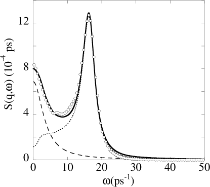
Figure 2: $S(q,\omega)$ for $q=0.29711$ a${}_{0}^{-1}$ at 395 K, from the model (solid line) and from MD (circles). The Rayleigh (broken line) and the Brillouin (dotted line) contributions to the model are also shown separately.

V Comparison of theories

An extensive body of work on the dynamics of liquids has been performed in the potential energy landscape and mode coupling theory research programs. In this Section we discuss those programs and compare our aims and results with theirs.

V.1 Potential Energy Landscape (PEL) Theories

Instantaneous normal modes (INM) were first reported in the MD calculations of Rahman et al. Rahman et al. (1976). These are the vibrational modes which diagonalize the potential energy curvature tensor at an arbitrary point on the potential energy surface. INM data are obtained by averaging over randomly chosen configurations on an equilibrium MD trajectory. Seeley and Keyes Seeley and Keyes (1989) argued that the INM averaged density of states contains information which may be used to construct theories of liquid state dynamics. The idea was applied to self diffusion Madan et al. (1990, 1991); Madan and Keyes (1993); Keyes (1994, 1995) by using INM data to estimate the hopping rate for Zwanzig’s approximation Zwanzig (1983). Bembenek and Laird Bembenek and Laird (1995, 1996) classified the imaginary frequency INM as unstable modes (double-well modes) and shoulder modes, and corresponding improvements in the fitting of calculated velocity autocorrelation functions followed Keyes et al. (1997); Li and Keyes (1997); Li et al. (1998); Li and Keyes (1999). Buchner, Ladanyi, and Stratt Buchner et al. (1992) started with the Hamiltonian for harmonic vibrations in a system of diatomic molecules, and showed that the INM description is accurate only for very short times, but that reasonable agreement is mantained for longer times if the imaginary frequency modes are omitted. A mean field theory was studied Wu and Loring (1992, 1993); Wan and Stratt (1994), as well as time evolution and mixing of INM David and Stratt (1998). Krämer et al. Krämer et al. (1998) showed that INM data at closely spaced points on the MD trajectory will give accurate results for the MD time correlation functions. To investigate the plane wave character of sound modes in liquid ZnCl₂, Ribeiro, Wilson and Madden Ribeiro et al. (1998) carried out an INM calculation of $S(q,\omega)$. This application of INM theory treats instantaneous configurations as if they were equilibrium configurations, hence the vibrational motion used is not a solution of the equations of motion (see Keyes and Fourkas Keyes and Fourkas (2000)). Additional INM calculations have been done for Rb Vallauri and Bermejo (1995), for Na Wu and Tsay (1996, 1998); Wu et al. (1998, 2000), and for water Cho et al. (1994); La Nave et al. (2000); Starr et al. (2001); La Nave et al. (2001).

In contrast to INM, quenched normal modes (QNM) are the vibrational modes evaluated at a local potential energy minimum (an equilibrium configuration). QNM data are usually obtained by averaging over the potential energy minima sampled from an equilibrium MD trajectory. For water at 300 K, Pohorille et al. Pohorille et al. (1987) found that the radial distribution calculated from QNM data are very similar to the MD results. Application of QNM theory to water was reviewed by Ohmine and Tanaka Ohmine and Tanaka (1993). Cao and Voth Cao and Voth (1995a, b) argued that, because of the thermal fluctuations, each potential energy valley must be replaced by a self-consistent temperature-dependent mean field. Notice this precludes a Hamiltonian formulation of liquid dynamics, because a Hamiltonian requires a time and temperature independent many-body potential. Several authors Gezelter et al. (1997); Keyes et al. (1998); Gezelter et al. (1998) discussed the issue of whether or not local information on the potential surface, embodied by the distribution of unstable instantaneous normal modes, can be used to predict the hopping rates and barrier heights for Zwanzig’s model Zwanzig (1983) of self diffusion. Rabani, Gezelter and Berne Rabani et al. (1997) introduced the cage correlation function, which measures the rate of change of atomic surroundings, and combined this with Zwanzig’s approximation to account for diffusion in LJ systems. For CS₂, these authors Gezelter et al. (1999) concluded that neither the INM nor the QNM density of states is the correct one to use in Zwanzig’s approximation. In the language of V-T theory, the cage correlation function aims to account for the mean transit-induced hopping motion of a single atom.

Currently the inherent structure (IS) research program is directed mainly toward supercooled liquids and the glass transition. The standard technique is to probe the potential energy surface by quenching at random times along the equilibrium MD trajectory for glass forming systems. The data collected this way are equilibrium statistical averages and depend on the temperature of the MD calculation. Systems studied include binary LJ mixtures, models for water, SiO₂, and orthoterphenyl. The binary LJ systems apparently do not crystallize, but do exhibit liquid behavior above an “effective” melting temperature $T_{m}$. For the Kob-Andersen binary system Kob and Andersen (1994), for example, $T_{m}\sim 1.0$, well above the mode-coupling critical temperature $T_{MCT}=0.435$ Sciortino et al. (2000). The following picture emerges. The average inherent structure energy is virtually constant for $T\gtrsim T_{m}$, but decreases as $T$ decreases below $T_{m}$ Sciortino et al. (1999); Sampoli et al. (2003); Sciortino et al. (2000); Büchner and Heuer (1999); Sastry (2000); Starr et al. (2001); Angelani et al. (2000); Sastry et al. (1998). Schrøder et al. Schrøder et al. (2000) presented numerical evidence that, below a crossover temperature in the vicinity of $T_{MCT}$, the system dynamics can be separated into vibrations around inherent structures and transitions between them. Potential energy saddle analyses also reveal this separation of system dynamics Angelani et al. (2000, 2002, 2003). Consensus is that the MD systems are in thermodynamic equilibrium at temperatures down to $T_{MCT}$. Structural entropy decreases toward zero as temperature decreases toward $T_{MCT}$ Sciortino et al. (1999, 2000); Sastry (2000); Scala et al. (2000); Sastry (2001); Saika-Voivod et al. (2001); Starr et al. (2001). The precise character of this decrease in structural entropy depends on the temperature-dependent distribution of the inherent structure energies Sciortino et al. (1999); Sampoli et al. (2003); Sciortino et al. (2000); Debenedetti et al. (2003); Büchner and Heuer (1999). The Gaussian character of this distribution at low temperatures has been established for binary LJ systems by numerical analysis, and has been shown on rather general arguments to result from the central limit theorem as $N\rightarrow\infty$ Heuer and Büchner (2000). Numerical confirmation of the Adams-Gibbs relation Adams and Gibbs (1965) between the decrease in structural entropy and the slowing down of structural relaxation has been obtained for several systems Scala et al. (2000); Sastry (2001); Saika-Voivod et al. (2001); Richert and Angell (1998). The key role of Adams-Gibbs in the IS theory of the glass transition is discussed by Shell and Debenedetti Shell and Debenedetti (2004). Recent work on ageing of the glass is of interest but beyond our present scope Mossa et al. (2002a); Sciortino and Tartaglia (2001); Donati et al. (2000); Kob et al. (2000).

V.2 Comparison of V-T and PEL theories

The goal of PEL theories is to describe statistical mechanical properties of liquids and supercooled liquids in terms of temperature-dependent statistical mechanical properties of the potential energy surface. INM and QNM theories work with temperature-dependent averages of vibrational mode data, and seek to explain time correlations such as velocity and density autocorrelations. IS theories work with temperature-dependent averages of structural potential energies and vibrational frequencies, and seek to explain such quantities as structural and vibrational entropy. In contrast, the goal of V-T theory is to construct a tractable and reasonably accurate zeroth order Hamiltonian, from which both equilibrium thermodynamic properties and time correlation functions can be calculated without adjustable parameters, and then proceed with Hamiltonian corrections to the zeroth order theory. Ultimately this is the most basic and comprehensive formulation available to theoretical physics.

The free energy in IS theory contains the important contribution $f_{basin}$, the free energy of the liquid constrained to be in one of its characteristic basins. The difficulties posed by this constraint are examined in detail by Sastry Sastry (2000), and Sciortino observes that there is no unique way to enforce the constraint Sciortino (2005). In contrast, V-T theory incorporates this constraint from the outset Wallace (1997a), in a manner consistent with all available experimental data, by replacing each random valley by its harmonic extension to infinity, with valley-valley intersections ignored. This formulation naturally separates in leading order and at all temperatures the intravalley vibrational motion and the intervalley transit motion Wallace (1997a), a separation later found in MD calculations at temperatures in the vicinity of $T_{MCT}$ Schrøder et al. (2000); Angelani et al. (2000, 2002, 2003). The V-T formulation also separates in leading order and at all temperatures the harmonic vibrational free energy from other free energy contributions, a separation again found in MD calculations for temperatures below melting Sciortino et al. (1999, 2000).

To test the predicted uniformity Wallace (1997a) of random valleys, we calculated the structural potential per atom and the vibrational frequency averages $\left<\omega\right>,\left<\omega^{2}\right>$ and $\left<\ln(\omega/\omega_{0})\right>$ for several monatomic random valleys with $N=500-3000$ Wallace and Clements (1999); Clements and Wallace (1999). The rms scatter was well below $0.01kT_{m}$ for the structural potential per atom, and was about $0.01\%$ of the mean for the vibrational frequency averages Wallace and Clements (1999); Clements and Wallace (1999). This scatter is negligible in V-T theory for $T\gtrsim T_{m}$. We also presumed that the scatter would vanish as $N\rightarrow\infty$. This limiting property is verified for the structural potential per atom by the analysis of Heuer and Büchner (see Eq. (14) with $M\rightarrow N$ of Heuer and Büchner (2000)).

As PEL theories develop, they are increasingly concerned with anharmonicity as it affects the interrelations among statistical mechanical averages Stratt (1995); David and Stratt (1998); Mossa et al. (2002b); La Nave et al. (2003). In the PEL approach, anharmonicity is taken to mean all atomic motion which is not harmonic vibrational motion. Anharmonicity therefore poses severe theoretical difficulties as soon as transits become important, i.e. at $T$ a little above $T_{MCT}$. Sciortino observes that there is currently no satisfactory model for anharmonicity at $T$ above $T_{MCT}$ Sciortino (2005). In contrast, V-T theory separates the correction to the zeroth order potential energy surface into two distinct contributions Wallace (1997a): (a) the boundary correction which subtracts the potential energy surfaces that were extended beyond the intersections of valleys, and (b) the anharmonic correction which is the anharmonic potential of each random valley up to its intersection with a neighboring valley. This is a most useful separation because the boundary correction to entropy is always negative, can be reasonably estimated, and is of increasing importance as temperature increases Wallace (1997a, 1998). The anharmonic free energy is quite complicated but, in our experience so far, it is always small in the liquid Wallace (1997a); Chisolm and Wallace (2004), just as it is in the crystal Wallace (2002).

Recent MD studies of complex systems exhibit behaviors characteristic of the V-T theory description of the potential surface. For a model of orthoterphenyl, the anharmonic entropy is very small at all $T$, the structural entropy is small and has very little temperature dependence, and the harmonic vibrational entropy is most of the total (85%) and has nearly all the temperature dependence (Fig. 12 of Mossa et al. (2002b)). These properties are very similar to the entropy contribution for all monatomic elemental liquids, as expressed in V-T theory Wallace (1997a, 1998). In addition, the excess of the mean potential energy over the harmonic vibrational contribution decreases for the binary LJ system at $T\gtrsim T_{m}$ (Fig. 5 of Broderix et al. (2000)). This decrease is present in all monatomic elemental liquids at $T\gtrsim T_{m}$, where it has been attributed to the boundary contribution Wallace (1997a, 1998).

That the random valleys dominate the statistical mechanics of monatomic liquids at $T\gtrsim T_{m}$ has been demonstrated by MD calculations (Figs. 1 and 2 of Wallace and Clements (1999)). Within the results of recent MD calculations for systems more complex than the monatomics, there is also strong evidence for the statistical mechanical dominance of macroscopically uniform (hence random) valleys at $T\gtrsim T_{m}$. The most prominent such evidence is (a) the mean inherent structure energy has very little temperature dependence at each fixed density for $T\gtrsim T_{m}$, and (b) the mean vibrational frequency distribution and its log moment are nearly independent of temperature at each fixed density for $T\gtrsim T_{m}$. Property (a) is found in monatomic LJ (Fig. 2 of Angelani et al. (2000)), in binary LJ systems (Fig. 1A of Sciortino et al. (1999)), Fig. 2A lower of Sampoli et al. (2003), Fig. 4 top of Sciortino et al. (2000), Fig. 8 of Büchner and Heuer (1999), Fig. 2 of Sastry (2000), Fig. 5 of Broderix et al. (2000), Fig. 1a of Sastry et al. (1998), Fig. 1a of Kob et al. (2000)) and in a model for water (Fig. 1b of Starr et al. (2001)). Property (b) is found in binary LJ systems (Figs. 6 and 7 of Sampoli et al. (2003), Fig. 10 of Büchner and Heuer (1999), Figs. 2a and 3 of Kob et al. (2000)) and in the model for water (Figs. 1b and 2c of Starr et al. (2001)). It therefore appears that the symmmetry classification of potential energy valleys as random and symmetric, with their associated properties, as introduced in V-T theory Wallace (1997a) is appropriate for liquids more complex than monatomics.

V.3 Comparison of V-T and Mode Coupling theories

Detailed summaries of mode coupling theories of liquid dynamics are given by Boon and Yip Boon and Yip (1980), Hansen and McDonald Hansen and McDonald (1986), and Balucani and Zoppi Balucani and Zoppi (1994). Applied to the glass transition, mode coupling theory predicts a dynamic singularity when temperature is lowered below the critical temperature $T_{MCT}$ Bengtzelius et al. (1984); Leutheusser (1984). From MD calculations for the binary LJ system, Kob and Andersen Kob and Andersen (1994, 1995a, 1995b) showed that mode coupling theory is able to rationalize the density correlation functions at low temperatures, in the vicinity of $T_{MCT}$. Further tests of mode coupling theory for glassy dynamics are reviewed by Götze Götze (1999). Mode coupling theory has been extensively applied to inelastic scattering in liquids at $T\gtrsim T_{m}$, and this is the application for which we shall compare mode coupling and V-T theories.

Mode coupling theory works with the generalized Langevin equation for $F(q,t)$, and expresses the memory function in terms of processes through which density fluctuations decay Boon and Yip (1980); Hansen and McDonald (1986); Balucani and Zoppi (1994). In the viscoelastic approximation, the memory function decays with a $q$-dependent relaxation time Boon and Yip (1980); Hansen and McDonald (1986); Balucani and Zoppi (1994). This approximation provides a good fit to the combined experimental data Copley and Rowe (1974) and MD data Rahman (1974a, b) for the Brillouin peak dispersion curve in liquid Rb Copley and Lovesey (1975) (see also Fig. 9.2 of Hansen and McDonald (1986)). Going beyond the viscoelastic approximation, Bosse et al. Bosse et al. (1978a, b) constructed a self-consistent theory for the longitudinal and transverse current fluctuation spectra, each expressed in terms of relaxation kernels approximated by decay integrals which couple the longitudinal and transverse excitations. This theory is in good overall agreement with extensive neutron scattering data and MD calculations for Ar near its triple point Bosse et al. (1978b). The theory was developed further by Sjögren Sjögren (1980a, b), who separated the memory function into a binary collision part, approximated with a Gaussian ansatz, and a more collective tail represented by a mode coupling term. For liquid Rb, this theory gives an “almost quantitative” agreement with results from neutron scattering experiments Copley and Rowe (1974) and MD calculations Rahman (1974a, b). More recently, inelastic x-ray scattering measurements have been done for the light alkali metals Li Scopigno et al. (2000a) and Na Scopigno et al. (2002a); Yulmetyev et al. (2003). These data have been analyzed by mode coupling theory, and the resulting fits to $S(q,\omega)$ are excellent, both for the experimental data and for MD calculations Scopigno et al. (2002a, b, c, 2000b, 2000c).

Recent results of V-T theory exhibit the following properties for the example of liquid sodium at melt. (a) The vibrational contribution alone, with no adjustable parameters, gives an excellent account of the Brillouin peak location at all $q$, and gives the natural width of the Brillouin peak, which is at least half the total width Wallace et al. . (b) The model described in Section IV, with two relaxation rates and a single multiplicative factor, can be made to fit $S(q,\omega)$ vs $\omega$ for a wide range of $q$, with relaxation rates near the transit rate as theoretically predicted De Lorenzi-Venneri and Wallace . The result illustrates the important point of comparison between V-T and mode coupling theories: the two methods are based on different decompositions of the physical processes involved. While mode coupling theory analyzes $F(q,t)$ in terms of processes by which density fluctuations decay, V-T theory analyzes $F(q,t)$ in terms of the two contributions to the total liquid motion, vibrations and transits. These two parts contribute to $S(q,\omega)$ as follows. (a) The extended random valley vibrational modes have infinite lifetimes, and represent no decay processes at all, yet they give the Brillouin peak its natural width. (b) In zeroth order where anharmonicity is neglected, transits are responsible for all genuine decay processes, and they contribute the entire width of the Rayleigh peak and part of the width of the Brillouin peak.

VI Summary and Discussion

The configuration part of an equilibrium statistical mechanical average can be thought of as an average over the many-particle potential energy surface. In V-T theory this average is constructed from integrals over individual potential energy valleys, where the entire contribution in the thermodynamic limit is from random valleys. Formally exact formulas are given for the canonical partition function in Eqs. (2) and (3), and for the time correlation function $\left<B(t)B^{*}(0)\right>$ in Eq. (8). For time-independent averages, which give the thermodynamic functions, the configuration contribution is the same for every random valley, as in Eq. (6). However, the same simplification does not hold for $\left<B(t)B^{*}(0)\right>$, because the system may be in a different random valley at time $t$ than at time $0$.

In a weighted integral over a random valley, the valley-valley intersections give only a small contribution, because these intersections are present in a relatively small part of configuration space. Hence in each such integral, only a small error is made when the actual random valley is replaced by its harmonic extension to infinity, and the integral is extended as well. We model the vibrational contribution to any equilibrium statistical mechanical average by that average evaluated for a system moving in one extended random valley. This model has no adjustable parameters, and can be evaluated for any temperature. The neglect of intervalley intersections, and the incidental neglect of anharmonicity, can be corrected for when necessary. The vibrational contribution to the partition function is written in Eq. (18), and to a time correlation function in Eq. (19).

By way of example, the vibrational contribution is studied for the dynamic response functions $F(q,t)$ and $S(q,\omega)$. The inelastic part in the one-mode approximation, $S_{vib}^{(1)}(q,\omega)$, consists of independent scattering from each of the complete set of normal vibrational modes. This scattering determines the location and natural width of the Brillouin peak. Vibrational theory is in near perfect agreement with MD calculations, Fig. 1.

In contrast to the thermodynamic functions, time correlation functions are strongly influenced by transits. Transits cause the system trajectory to move among random valleys, and in the dynamical variable $B(t)B^{*}(0)$, each transit contributes to the decorrelation of $B(t)$ with $B^{*}(0)$. A simple approximation for $F(q,t)$, Eq. (41), preserves this effect in the atomic equilibrium positions, but neglects it in the atomic displacements. This approximation yields two results: (a) while with vibrational motion alone we have $F_{vib}(q,\infty)>0$, when transits are present we have $F_{liq}(q,\infty)=0$, and (b) while with vibrational motion alone the Rayleigh peak has zero width and the Brillouin peak has its nonzero natural width, the effect of transits is to broaden both peaks without shifting them. These transit properties are incorporated into a parametrized model, Eqs. (42-46), which is capable of accounting for MD calculations of $S(q,\omega)$ in the liquid Fig. 2.

V-T theory rests on a new analysis of the many-body potential energy surface underlying the motion of a monatomic liquid, namely the symmetry classification of valleys and the statistical dominance and microscopic uniformity of the random valleys. The same potential surface is then appropriate for supercooled liquid and glass states. The glass corresponds to very small transit rate Wallace (1999), vanishing on the timescale of dynamic response experiments, so property (a) of the preceding paragraph implies that $F(q,\infty)$ is positive for the glass. This result has been observed for real glasses Mezei (1989) and also for computer models of glasses Brakkee and de Leeuw (1989, 1990). From V-T theory, the value of this positive constant is $F_{vib}(q,\infty)$ for an extended random valley. It has also been shown previously that a vibrational analysis agrees with MD calculations for $S(q,\omega)$ in a LJ glass Mazzacurati et al. (1996); Ruocco et al. (2000). The similar result for sodium is shown here in Fig. 1, where the vibrational theory is specifically for an extended random valley. Then, according to V-T theory, this vibrational contribution has application to the liquid state, and leads to the result shown in Fig. 2.

Finally, we have also compared and contrasted our results with those of the potential energy landscape (PEL) and mode coupling theory (MCT) approaches to liquid dynamics. The various types of PEL theory seek to describe the statistical mechanics of liquids in terms of temperature-dependent properties of their potential energy surfaces, while MCT describes the liquid in terms of different treatments of the Langevin equation for $F(q,t)$. In contrast, our goal is to produce a theory with an accurate and tractable zeroth order Hamiltonian, from which equilibrium and nonequilibrium quantities can be computed without adjustable parameters, and then make corrections to this Hamiltonian. In so doing, we have predicted and verified several significant properties of the potential energy surface, such as the classification of valleys described in the previous paragraph, making the analysis of liquid dynamics considerably simpler. We have then identified two distinct corrections to the zeroth order Hamiltonian, namely the boundary correction which accounts for valley-valley intersections, and the anharmonicity of the random valleys. Of these two, the boundary correction is by far the most important, and is not too difficult to estimate. This helps address a significant problem faced recently by PEL theories. Further, some studies in the PEL program are revealing properties of the potential energy surface predicted by V-T theory independently of our efforts. In contrasting our treatment of $F(q,t)$ with MCT, we noted that our theories are based on different decompositions of the relevant physical processes: MCT analyzes $F(q,t)$ in terms of the decay of density fluctuations, while V-T analysis is in terms of the two contributions to the actual motion of particles in a liquid, vibrations and transits. We argue that the direct connection of this analysis to the motion of the particles, which is of universal applicability to all equilibrium and nonequilibrium quantities, provides a basis for a unified treatment of all processes in the liquid and supercooled states.

There is much still to learn about the physical nature of transits. We have observed from the outset that transits must be “correlation controlled,” and not just thermally activated Wallace (1997a). This is because, as mentioned above, the valley-valley intersections are present in a relatively small part of configuration space, so that the transit rate is limited by the time required for the system to find a transit pathway. The highly correlated motion of the atoms involved in a transit is revealed in MD calculations Wallace et al. (2001). Hence transits provide a new and challenging problem in the motion of many particle systems, and the solution of this problem will have a key role in the nonequilibrium properties of liquids, through their time correlation functions.