Dynamics of a Tonks-Girardeau gas released from a hard-wall trap

Abstract

We study the expansion dynamics of a Tonks-Girardeau gas released from a hard wall trap. Using the Fermi-Bose map, the density profile is found analytically and shown to differ from that one of a classical gas in the microcanonical ensemble even at macroscopic level, for any observation time larger than a critical time. The relevant time scale arises as a consequence of fermionization.

The Tonks-Girardeau (TG) regime Girardeau60 is that of 1D impenetrable bosons, which is relevant to atom waveguide experiments with low densites and temperatures and large scattering lengths Olshanii98 . Under such conditions the radial degrees of freedom are reduced to zero-point oscillations, resulting a 1D effective system, as it has been demonstrated in several experiments exp . Some remarkable studies dealing with dynamics in this regime have shown the limits of mean-field theory in splitting-recombination processes GW05bis , the spatial focusing of the probability density through Talbot oscillations RCB99 , and existence of dark and grey solitons in a toroidal trap GW00 . During the 1D expansion of a harmonically confined Tonks gas, fermionization of the system was observed in the momentum distribution MG05 ; OS02 . A parallel study pointing out the “reciprocal” character of the Fermi-Bose duality, was recently carried out in GM05 for a fermionic TG gas which undergoes a dynamical bosonization. In the mean time, and motivated by the experimental build-up of square well HHHR01 and hard wall optical box traps MSHCR05 a growing interest has been developed concerning low dimensional Bose gases trapped in such geometries Cazalilla02 ; BGOL05 after the seminal paper by Gaudin Gaudin71 . However, most of the studies have dealt with the gas within the trap and, at variance with the case of a harmonic confinement, only the single-particle evolution has been considered, in the field of ultracold neutron interferometry GK76 and diffraction in time Godoy02 .

In this Letter we account for a detailed study of the expansion dynamics of a TG gas, after switching off the confining hard wall potential and show the deviation from the associated classical gas in the microcanonical ensemble. In such a regime the Fermi-Bose (FB) map Girardeau60 ; YG05 ; CS99 ; GW00b gives the many body wavefunction of $N$ strongly interacting bosons from the one of a free Fermi gas with all spins frozen in the same direction. In order to do so, it suffices to apply the “antisymmetric unit function” $\mathcal{A}=\prod_{1\leq j<k\leq N}sgn(x_{k}-x_{j})$, as $\psi_{B}(x_{1},\dots,x_{N})=\mathcal{A}(x_{1},\dots,x_{N})\psi_{F}(x_{1},\dots,x_{N}).$ The Fermi wavefunction, antisymmetric under permutation of particles, is built as a Slater determinant, with one particle in each eigenstate of the trap

$$\psi_{F}(x_{1},\dots,x_{N})=\frac{1}{\sqrt{N!}}det_{n,k=1}^{N}\phi_{n}(x_{k}).$$ (1)

One more advantage of the general FB mapping is that it holds for time dependent processes (governed by one-body external potentials), since the $\mathcal{A}$ operator does not include time explicitly GW00b ; YG05 , this is, Fermi statistics holds under time evolution. The glaring upshot is that as far as local coordinate distributions are concerned, to deal with the manybody Tonks gas it suffices to work out the single particle problem, since $|\psi_{B}(x_{1},\dots,x_{N};t)|^{2}=|\psi_{F}(x_{1},\dots,x_{N};t)|^{2}$. In particular, from the involutivity of the $\mathcal{A}$ operator ($\mathcal{A}^{2}=1$) and the fact that $\langle\phi_{n}|U^{{\dagger}}U|\phi_{m}\rangle=\delta_{nm}$, where $U$ is the time-evolution operator, it follows that the time-dependent density profile can be calculated as GW00b

$$\rho(x,t) = N\!\!\int|\psi_{B}(x,x_{2},\dots,x_{N};t)|^{2}dx_{2}\cdots dx_{N}$$ (2)

$$= \sum_{n=1}^{N}|\phi_{n}(x,t)|^{2}.$$

Single eigenmode dynamics. Motivated by the Eq. (2), in this section we tackle the problem of studying the time evolution of the $n$-th eigenstate of a hard wall trap. As it is well-known they have the general form $\phi_{n}(x,t=0)=\sqrt{\frac{2}{L}}\sin(n\pi x/L)\chi_{[0,L]}(x)$, with $n\in\mathbf{N}$ where the characteristic function can be conveniently written as a difference of Heaviside functions, $\chi_{[0,L]}(x)=\Theta(L-x)-\Theta(-x)$. Concerning the dynamics we consider the free evolution under the propagator

$$K(x,t|x^{\prime},0)=\sqrt{\frac{m}{2\pi i\hbar t}}e^{\frac{im(x-x^{\prime})^{2}}{2t\hbar}}$$ (3)

after suddenly switching off the trap at zero time. Using the superposition principle and introducing $p_{n}=\hbar n\pi/L$,

$$\phi_{n}(x,t) = \int_{-\infty}^{\infty}dx^{\prime}K(x,t|x^{\prime},t=0)\psi(x^{\prime},t^{\prime}=0)$$ (4)

$$= \frac{1}{2i}\sqrt{\frac{2}{L}}\sum_{\alpha=\pm}\alpha\big{[}e^{i\alpha p_{n}L/\hbar}M(x-L,\alpha p_{n}/\hbar,\hbar t/m)$$

$$-M(x,\alpha p_{n}/\hbar,\hbar t/m)\big{]}$$

with

$$M(x,p/\hbar,\hbar t/m):=\int_{-\infty}^{0}dx^{\prime}K(x,t|x^{\prime},t^{\prime}=0)e^{ipx^{\prime}/\hbar}$$

$$=\frac{e^{i\frac{mx^{2}}{2t\hbar}}}{2}w\bigg{[}-\frac{1+i}{2}\sqrt{\frac{t}{m\hbar}}\left(p-\frac{mx}{t}\right)\bigg{]},$$ (5)

and $w(z)=e^{z^{2}}erfc(-iz)$ the so called Faddeyeva function Faddeyeva . After Moshinsky52 , $M(x,k,\tau)$ has been named the Moshinsky function. Similar expressions have been derived in the field of ultracold neutron interferometry GK76 , and discussed recently in the context of diffraction in time Godoy02 .

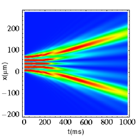
Figure 1: Density plot of the probability density for the dynamical evolution for the fifth eigenstate (⁸⁷Rb atom, $L=80\mu m$).

When the particle is trapped in the $n$-th mode, and at short times after being released, the probability density presents $n$ maxima, but the central ones tend to fade away with time as shown in Fig. 1. Indeed, the general structure of the $n$-th eigenstate ($n>1$) under evolution presents a bifurcation in two main branches after the semiclassical time $t_{n}=mL/(2p_{n})=mL^{2}/(2n\pi\hbar)$.

Tonks gas dynamics. Remarkably, as stated above, the calculation of the density profile is possible from Eqs. (2),(4), and (Dynamics of a Tonks-Girardeau gas released from a hard-wall trap). As illustrated in Fig. 2, the density profile exhibits at short times a peaked structure with the number of maxima equal to that of particles.

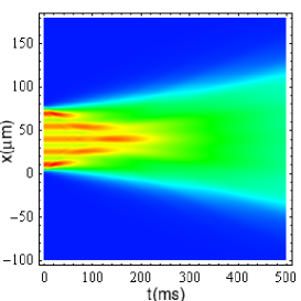
Figure 2: Density plot of the probability density $\rho$ for a Tonks gas composed of $N=5$ atoms of ⁸⁷Rb ($L=80\mu m$).

This spatial antibunching results from the underlying fermionization characteristic of the Tonks regime. Indeed, the two-particle local correlation, $g_{2}=\langle\hat{\Psi}^{{\dagger}}(x)^{2}\hat{\Psi}(x)^{2}\rangle/\langle\hat{\Psi}^{{\dagger}}(x)\hat{\Psi}(x)\rangle^{2}$, was shown to tend to zero even for non-zero temperatures KGDS03 . However, the visibility of the interference pattern is lost both with increasing time and the number of bosons under consideration.

A measure of the roughness of the density profile is the root mean square of the density profile weighted with itself, $\sigma_{\rho_{N}}=\sqrt{\langle\rho_{N}\rangle_{\rho_{N}}^{2}-\langle\rho_{N}^{2}\rangle_{\rho_{N}}}$, with $\rho_{N}$ the density profile normalised to one particle. In fact, at time equals zero and as a function of the particle number this measure decreases monotonically as shown in Fig. 3a, in agreement with the resolution of the identity within the box, $lim_{N\rightarrow\infty}\rho={\bf 1}_{[0,L]}$, see Eq. (2).

Figure 3: a) Dependence of the variance on the number of ⁸⁷Rb atoms for the density profile of TG gas confined in a trap. b) Time dependence of the variance of the density profile for different number of ⁸⁷Rb atoms. Filled circles mark the corresponding $t_{N}$ and $L=80\mu m$.

The time evolution is richer in structure, presenting an initial positive slope, see Fig. 3b, to finally start to decrease after $t\sim t_{N}$, reaching zero asymptotically.

After a transient regime, where the structure of the peaks varies in time, the roughness of the density profile becomes monotonically decreasing with both time and number of particles. In particular, the fastest components will be associated with the highest excited state (the Fermi level in the dual system of non-interacting spin-frozen fermions), and therefore with quasi-momentum given by $\pm p_{N}=\pm\hbar N\pi/L$. Actually, these components govern the width of the expanding cloud for $t\gtrsim t_{N}$. Figure 4 shows the variation in time of the full width at half maximum (FWHM) for different number of particles.

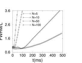
Figure 4: Time dependence of the FWHM of a cloud of ⁸⁷Rb atoms released from a trap $80\mu m$ in width.

The upshot is that deviations from a linear dependence on time are observed right after switching off the trap, similarly to the results reported in OS02 for the harmonically confined Tonks gas. Such deviations disappear with increasing number of particles and already for $N\sim 100$ are bellow the millisecond time scale. From its definition, one can conclude that $t_{N}$, the time necessary for a classical particle to leave the trap when it is initially located in the center of the box and moves with the momentum $p_{N}$, arises as a consequence of fermionization. Nevertheless, it is clear from the transient features of the single-particle solution that a self-similar expansion does not occur for a TG gas released from a hard wall trap. This fact contrasts with the harmonic case, pointing out the relevance of the confining geometry.

Comparison with a classical gas. Next we consider a classical gas of distinguishable particles interacting through a contact potential. Since for the TG gas the total energy ($E=\sum_{n=1}^{N}E_{n},E_{n}=\hbar^{2}n^{2}\pi^{2}/(2mL^{2})$) is fixed once the number of particles $N$ in the initial trap is specified BGOL05 , it is natural to deal with a microcanonical ensemble in the classical limit. This leads to a distribution in phase space of the form:

$$\rho_{cl}({\bf x},{\bf p},0;E)=\mathcal{N}_{0}\delta\left(E-\sum_{i=1}^{N}\frac{p_{i}^{2}}{2m}\right)\prod_{i=1}^{N}\Theta(x_{i})\Theta(L-x_{i}),$$ (6)

where the normalization reads $\mathcal{N}_{0}=N\Gamma(N/2)/(2m\pi^{N/2}L^{N}\varrho^{N-1})$, $\Gamma(z)$ is the Gamma function and $\varrho=\sqrt{2mE}$. Using Liouville’s theorem, momentum conservation (but for interchange), and the symmetry under permutation of particles in the microcanonical ensemble, one finds $\rho_{cl}({\bf x},{\bf p},t;E)=\rho_{cl}({\bf x}-{\bf p}t/m,{\bf p},0;E)$, where ${\bf x}=\{x_{1},\cdots,x_{N}\}$, and ${\bf p}=\{p_{1},\cdots,p_{N}\}$. To obtain the density profile, an integration over $\{x_{2},\dots,x_{N},p_{1},\dots,p_{N}\}$ variables has to be performed. Note that each of the integrals over $x_{i}$ contributes exactly $L$. Moreover, all the integrals over momenta can be carried out by using the generalisation of spherical polar coordinates to a hypersphere in a $N$-dimensional space subjected to the constraint $\sum_{i}p_{i}^{2}=\varrho^{2}=2mE$ Sommerfeld49 ; MW95 , which fixes the radius $\varrho$ of the hypershell. Since it is always possible to choose one coordinate of the form $p=p_{1}=\varrho\cos\xi$, it follows that

$$\rho_{cl}(x,t;E) = \mathcal{N}\int_{0}^{\pi}d\xi\sin^{N-2}\xi\Theta(x-t\varrho\cos\xi/m)$$ (7)

$$\times\Theta(L+t\varrho\cos\xi/m-x),$$

where $\mathcal{N}=N\Gamma(N/2)/(\sqrt{\pi}L\Gamma[(N-1)/2])$ is the normalisation constant.

For a systematic comparison between the Tonks and microcanonical gas, we introduce the time-dependent measure $D_{N}(t)=\int dx|\rho(x,t)-\rho_{cl}(x,t)|/N$, which is plotted in Fig. 5 for different number of particles.

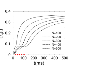
Figure 5: Measure $D_{N}$ for a fixed density, $d_{0}=1$ atom$/\mu m$ and increasing number of particles (⁸⁷Rb). Filled circles mark $t_{N}$ and verify $D_{N}(t_{N})\simeq 0.08$.

As a result, a clear time scale given by $t_{N}$ can be established, such that for small times ($t/t_{N}<1$) both quantum and classical profiles essentially coincide ($D_{N}<0.1$).

In particular, the microcanonical model reproduces for short times and low number of particles the quantum profile in a coarse-grained fashion, neglecting inteference (see Fig.6a). It is precisely for low $N$ when the differences between the initial quantum spatial distribution and the uniform classical one, are greater. For larger number of particles the quantum profile tends to “resolve the identity” within the trap, reaching a uniform constant distribution when $N\rightarrow\infty$. This is, the quantum result is a staggeringly flat distribution but for the smoothed edges, and can be understood as a consequence of the discrete spectrum of the free Hamiltonian confined in the subspace $[0,L]$, with equally spaced quasimomenta $p_{n}$ (See Fig.1 ). Indeed, in the limit $t/t_{N}\ll 1$ and $N\gg 1$, the profile is well described by the characteristic function of the form $\Theta(x+p_{F}t/m)\Theta(L+p_{F}t/m-x)/(L+2p_{F}t/m)$ (Fermi-hat), which expands with the momentum of the Fermi level in the dual system, $p_{N}$. Similar profiles have already been reported for an effective 1D weakly interacting fermionic gas confined in a harmonic trap ID05 .

By contrast, it can be proved that the momentum distribution of the microcanonical gas is of the form MW95

$$f_{cl}^{(N)}(p)=\frac{\Gamma(N/2)}{\sqrt{\pi\varrho^{2}}\Gamma((N-1)/2)}\left(1-\frac{p^{2}}{\varrho^{2}}\right)^{(N-3)/2}$$ (8)

which in the reduced variable $p/\varrho$, for large $N$, tends to be a Gaussian with zero mean and $1/N$ variance. It follows that the density profile becomes also Gaussian in this limit, in clear disagreement with the TG profile, as shown in Fig. 5 for $t>t_{N}$.

In the thermodynamic limit, achieved at a given observation time and fixed density $d_{0}=N/L$ by taking $N\rightarrow\infty$, both the quantum and microcanonical density profiles become indistinguishable of one another.

Figure 6: Microcanonical (dashed lines) and quantum (continuous line) density profiles 100ms after expansion for: a) fixed length box $L=80\mu m$, and $N(t_{N})$=10 (137ms), 25 (55ms), 50 (27ms), and 100 (1ms), from top to bottom. b) fixed density $d_{0}=1$atom$/\mu m$, and $N(t_{N})$ =100 (21ms), 250 (54ms), 500 (107ms), and 2000 (428ms), from bottom to top.

Since for fixed density $t_{N}=mN/(2\pi\hbar d_{0}^{2})$, the agreement is reached more easily at short times after switching off the trap. Figure 6b shows that at an observation time of $100\mu s$, 2000 particles suffice. Deviation from the classical gas increases with time which acts as a lense pointing out the difference in the underlying momentum distributions. Indeed, taking note of the experimental number of atoms in MSHCR05 , generally between 500-3500, a rectangular profile is to be expected in the TG regime both in the trap and after switching it off, being overall described by the Fermi-hat model.
Discussion. Taking advantage of the Fermi-Bose map, the dynamics of a strongly interacting many-body system can be worked out once the time evolution of the single-particle eigenstates of the confining hard-wall trap is known. In this way, we have accounted for the first study of a many-body Moshinsky shutter problem Moshinsky52 ; DM05 ; GCR97 including interactions. Right after switching off the trap, the profile evolves through a transient regime where the overall behaviour is analogous to the one of a classical gas in the microcanonical ensemble.

However, at times $t>t_{N}=mL^{2}/(2N\pi\hbar)$ and in the same conditions $(N,L)$, a regime with uniform density is observed in the Tonks gas, clearly deviating from the classical bell-shaped profile. The origin of this main feature can be traced back to the discrete spectrum of the original trap potential. Finally, it is noteworthy that the results obtained in this Letter equally hold for a noninteracting Fermi gas due to the involutivity of the antisymmetric unit function which entails the 1D Fermi-Bose duality.

- (1) M. Girardeau, J. Math. Phys. 1 516, (1960).
- (2) M. Olshanii, Phys. Rev. Lett. 81 938, (1998); V. Dunjko, V. Lorent, and M. Olshanii, ibid 86, 5413 (2001).
- (3) B. Paredes et al Nature (London) 429, 227 (2004); T. Kinoshita et al., Science 305, 1125 (2004).
- (4) M. D. Girardeau and E. M. Wright, Phys. Rev. Lett. 84 5239 (2005).
- (5) A. Rojo, J. L. Cohen, and P. R. Berman, Phys. Rev. A 60 1482 (1999).
- (6) M. D. Girardeau and E. M. Wright, Phys. Rev. Lett. 84, 5239 (2000).
- (7) A. Minguzzi and D. M. Gangardt, Phys. Rev. Lett. 94, 240404 (2005).
- (8) P. Öhberg and L. Santos, Phys. Rev. Lett. 89, 240402 (2002).
- (9) M. D. Girardeau and A. Minguzzi, cond-mat/0508063 (2005).
- (10) W. Hänsel et al., Nature 413, 498 (2001).
- (11) T. P. Meyrath, F. Schreck, J. L. Hanssen, C-S. Chuu, and M. G. Raizen, Phys. Rev. A R71, 041604 (2005).
- (12) M. A. Cazalilla, Europhys. Lett. 59, 793 (2002); M. A. Cazalilla, J. Phys. B 37, S1 (2004).
- (13) M. T. Batchelor et al., J. Phys. A 38, 7787 (2005).
- (14) M. Gaudin, Phys. Rev. A 4, 386 (1971).
- (15) A. S. Gerasimov and M. V. Kazarnovskii, Sov. Phys. JETP 44, 892 (1976).
- (16) S. Godoy, Phys. Rev. A 65, 042111 (2002).
- (17) V. I. Yukalov and M. D. Girardeau, Laser Phys. Lett 2, 375 (2005).
- (18) T. Cheon and T. Shigehara, Phys. Rev. Lett. 82, 2536 (1999).
- (19) M. D. Girardeau and E. M. Wright, Phys. Rev. Lett. 95, 010406 (2005)
- (20) M. D. Girardeau and E. M. Wright, Phys. Rev. Lett. 84, 5691 (2000).
- (21) V. N. Faddeyeva and N. M. Terentev Mathematical Tables: Tables of the values of the function for complex argument, Pergamon, New York (1961); A. Abramowitz and I. A. Stegun Handbook of Mathematical Functions, Dover, New York (1965).
- (22) M. Moshinsky, Phys. Rev. 84, 525 (1951); M. Moshinsky, ibid 88, 625 (1952).
- (23) A. Sommerfeld, Partial Differential Equations in Physics, Academic, New York, p.227 (1949).
- (24) J. G. Muga and D. M. Wardlaw, Phys. Rev. E 51, 5377 (1995).
- (25) K. V. Kheruntsyan, D. M. Gangardt, P.D. Drummond, and G. V.Shlyapnikov, Phys. Rev. Lett. 91, 040403 (2003).
- (26) A. Imambekov and E. Demler, cond-mat/0510801.
- (27) A. del Campo and J. G. Muga, J. Phys. A 38, 9803 (2005).
- (28) G. García-Calderón and A. Rubio, Phys. Rev. A 55, 3361 (1997).