Statistical descriptions of nonlinear systems at the onset of chaos

Abstract

Ensemble of initial conditions for nonlinear maps can be described in terms of entropy. This ensemble entropy shows an asymptotic linear growth with rate $K$. The rate $K$ matches the logarithm of the corresponding asymptotic sensitivity to initial conditions $\lambda$. The statistical formalism and the equality $K=\lambda$ can be extended to weakly chaotic systems by suitable and corresponding generalizations of the logarithm and of the entropy. Using the logistic map as a test case we consider a wide class of deformed statistical description which includes Tsallis, Abe and Kaniadakis proposals. The physical criterion of finite-entropy growth $K$ strongly restricts the suitable entropies. We study how large is the region in parameter space where the generalized description is useful.

I Introduction

Sensitivity to initial conditions in chaotic systems has an exponential asymptotic regime in fully-chaotic regions and a power-law regime in transition regions. A description in terms of generalized exponentials leading to the definition of generalized Lyapunov exponents gives an unified framework for both regimes Tsallis:1997 ; Tonelli:2004ha . For instance, if Tsallis’ generalization is used: the sensitivity $\xi\equiv\lim_{\Delta x(0)\to 0}\Delta x(t)/\Delta x(0)$ grows asymptotically as the generalized exponential $\widetilde{\exp}(\lambda t)$, where $\widetilde{\exp}(x)=\exp_{q}(x)\equiv[1+(1-q)x]^{1/(1-q)}$; the exponential behavior for the chaotic regime is recovered for $q\to 1$: $\lim_{q\to 1}\exp_{q}(\lambda_{q}t)=\exp(\lambda t)$. A large class of generalized exponentials shows similar behavior Tonelli:2004ha .

The statistical definition of entropy production rate, where an ensemble of initial conditions confined to a small region is let evolve and the entropy is a functional of the occupation numbers of an appropriate partition, shows close analogy to the production rate of thermal entropy and appears to coincide with the Kolmogorov-Sinai entropy in chaotic regimes Latora:1999prl .

This rate of loss of information can be also suitably generalized to include both full-chaotic and edge-of-chaos cases. At the edge of chaos the statistical description is recovered with the generalized entropic form proposed by Tsallis Tsallis:1987eu $S_{q}=(1-\sum_{i=1}^{N}p_{i}^{q})/(q-1)$, which grows linearly for a specific value of the entropic parameter $q$ characteristic of the system: $\lim_{t\to\infty}\lim_{L\to 0}S_{q}(t)/t=K_{q}$, where $S_{q}$ reduces to $-\sum_{i=1}^{N}p_{i}\log p_{i}$ in the limit $q\to 1$, $p_{i}$ being the fraction of the ensemble found in the $i$-th cell of linear size $L$. As a matter of fact a large class of entropies, which includes Tsallis’one, reproduces this asymptotic linear behavior Tonelli:2004ha ; Lissia:2005by . The asymptotic power law behavior (exponent) that characterizes the entropy growth is the same that describes the asymptotic power-law sensitivity to initial conditions Latora:1999vk ; Tonelli:2004ha ; Lissia:2005by .

Finally, it has been also conjectured that the relationship between the asymptotic entropy-production rate $K$ and the Lyapunov exponent $\lambda$ for chaotic systems (the Pesin-like identity : $K=\lambda$) can be extended to systems at the edge of chaos $K_{q}=\lambda_{q}$ Tsallis:1997 .

There exist numerical evidences supporting this framework with the entropic form $S_{q}$ for the logistic Tsallis:1997 and generalized logistic-like maps Tsallis:1997cl . The linear behavior of the generalized entropy for specific choices of $q$ has been observed for two families of one-dimensional dissipative maps Tirnakli:2001 .

Evidence exists also for a more generalized coherent statistical framework, which includes Tsallis’ proposal Tonelli:2004ha ; Lissia:2005by ; Kaniadakis:2004td . The generalized entropic form is $-\sum_{i=1}^{N}p_{i}\widetilde{\log}(p_{i})$, where $\widetilde{\log}$ indicates the following two-parameter family Mittal ; Taneja1 ; Borges1 ; Kaniadakis:2004nx ; Kaniadakis:2004ri of logarithms

$$\widetilde{\log}(\xi)\equiv\frac{\xi^{\alpha}-\xi^{-\beta}}{\alpha+\beta}\quad,$$ (1)

where $\alpha$ ($\beta$) characterizes the large (small) argument asymptotic behavior; in particular, $\widetilde{\exp}(\lambda t)\equiv\widetilde{\log}^{-1}(\lambda t)\sim(\lambda t)^{1/\alpha}$ for large $t$. The requirements Naudts1 that the logarithm be an increasing function, therefore invertible, with negative concavity (the related entropy is stable), and that the exponential be normalizable for negative arguments select $0\leq\alpha\leq 1$ and $0\leq\beta<1$ Kaniadakis:2004td ; solutions with negative $\alpha$ and $\beta$ are duplicate, since the family (1) possesses the symmetry $\alpha\leftrightarrow-\beta$.

Renormalization-group methods have been used Baldovin:2002a ; Baldovin:2002b to demonstrate that the asymptotic behavior of the sensitivity to initial conditions in the logistic and generalized logistic maps is bounded by a specific power-law whose exponent could be determined analytically for initial conditions on the attractor. For evolution on the attractor the connection between entropy and sensitivity has been studied analytically and numerically for Tsallis’ entropic form Baldovin:2004 .

Sensitivity and entropy production have been studied in one-dimensional dissipative maps using ensemble-averaged initial conditions chosen uniformly over the interval embedding the attractor Ananos:2004a : the statistical picture, i.e., the relation between sensitivity and entropy exponents and the generalized Pesin-like identity, has been confirmed. Indeed the ensemble-averaged initial conditions appear more relevant for the connection between ergodicity and chaos and for practical experimental settings.

The main objective of the present work is to review the general validity of the above-described picture, including the generalized Pesin-like identity, and the physical criterion of finite-entropy production per unit time (linear growth), which strongly selects appropriate entropies and fixes their parameters. In addition we specifically study how large is the transition region where the generalized formalism is useful, before the usual exponential regime sets in.

II Statistical description

From our investigation on the entire class of logarithms in Eq. (1), we review results for the following one-parameter cases:

(1) Tsallis’ seminal proposal Tsallis:1987eu : $\alpha=1-q$ and $\beta=0$;

(2) the $\gamma$ logarithm : $\alpha=2\beta=2\gamma$;

(3) the Abe logarithm: $\beta=\alpha/(1+\alpha)=1-q_{A}$, named after the entropy introduced by Abe Abe:1997qg , which possesses the symmetry $q_{A}\to 1/q_{A}$;

(4) the Kaniadakis logarithm: $\alpha=\beta=\kappa$, which shares the same symmetry group of the relativistic momentum transformation and has applications in cosmic-ray and plasma physics Kaniadakis:2001nl ; Kaniadakis:2002sr ; Kaniadakis:2005zk .

Our laboratory is the logistic map $x_{i+1}=1-\mu x^{2}_{i}$, at and near the infinite bifurcation point $\mu_{\infty}=1.401155189$. If the sensitivity follows a deformed exponential $\xi(t)=\widetilde{\exp}(\lambda t)$, analogously to the chaotic regime when $\xi(t)\sim\exp(\lambda t)$, the corresponding deformed logarithm of $\xi$ should yield a straight line $\widetilde{\log}(\xi(t))=\widetilde{\log}(\widetilde{\exp}(\lambda t))=\lambda t$.

Starting from an initial condition $x_{0}$, the sensitivity has been obtained, $\xi(t)=(2\mu)^{t}\prod_{i=0}^{t-1}|x_{i}|$, for $1\leq t\leq 80$; the generalized logarithm $\widetilde{\log}(\xi)$ has been averaged over a sample of $4\times 10^{7}$ random initial conditions $-1<x_{0}<1$. The averaging over initial conditions, $\langle\cdots\rangle$, is appropriate for a comparison with the entropy production.

For each of the generalized logarithms, $\langle\widetilde{\log}(\xi(t))\rangle$ has been fitted to a quadratic function for $1\leq t\leq 80$ and $\alpha$ has been chosen such that the coefficient of the quadratic term be zero; in fact $\widetilde{\log}(\xi)$ linear in $t$ means that the sensitivity $\xi$ behaves as $\widetilde{\exp}(\lambda t)$: we label this value $\alpha^{\mathrm{av}}_{\mathrm{sens}}$.

In fact, the exponent obtained with this procedure has been denoted $q_{\mathrm{sens}}^{\mathrm{av}}$ in the case of Tsallis’ entropy Ananos:2004a and it is different from $q_{\mathrm{sens}}$ obtained by choosing the initial condition $x_{0}$ (fixed point of the map) Baldovin:2004 .

The values of $\alpha^{\mathrm{av}}_{\mathrm{sens}}$ corresponding to the four different choices of the logarithm are (1) 0.644, (2) 0.656, (3) 0.657, and (4) 0.653 with a statistical errors of 0.002, calculated by repeating the fitting procedure for sub-samples, and a systematic error of $0.004$, estimated by fitting over different ranges of $t$. The exponent of Tsallis’ formulation $\alpha^{\mathrm{av}}_{\mathrm{sens}}=0.644\pm 0.002$ is consistent with the value of Ref. Ananos:2004a $q^{\mathrm{av}}_{\mathrm{sens}}=1-\alpha^{\mathrm{av}}_{\mathrm{sens}}\approx 0.36$. The values of $\alpha^{\mathrm{av}}_{\mathrm{sens}}$ obtained using the four different formulations are within $\pm 1\%$: the common asymptotic behavior (deviations at the 1% level are due to the inclusion in the global fitting of small values of $\xi$) is $\alpha^{\mathrm{av}}_{\mathrm{sens}}=0.650\pm 0.005$.

Figure 1 shows the straight-line behavior of $\widetilde{\log}(\xi)$ for $\alpha=\alpha^{\mathrm{av}}_{\mathrm{sens}}$: the corresponding slopes $\lambda$ (generalized Lyapunov exponents) are (1) $0.271\pm 0.003$, (2) $0.198\pm 0.002$, (3) $0.185\pm 0.002$, and (4) $0.148\pm 0.001$ from top to bottom; an additional systematic error of about 0.003 has been estimated by different choices of the range of $t$. While the values of $\alpha$ are consistent with a universal exponent independent of the particular deformation, the slope $\lambda$ strongly depends on the choice of the logarithm.

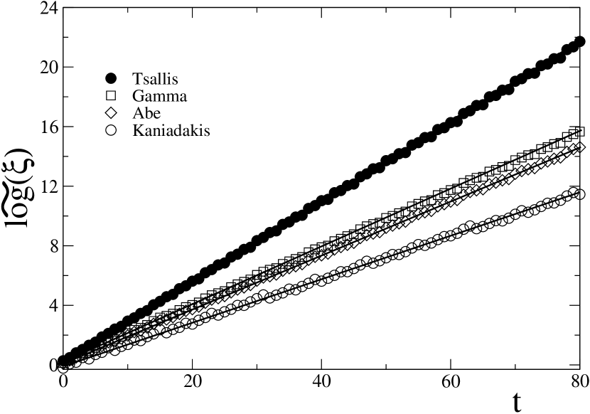
Figure 1: Generalized logarithms $\widetilde{\log}(\xi)$, see Eq. (1), of the sensitivity to initial conditions averaged over $4\times 10^{7}$ uniformly distributed initial conditions as function of time. From top to bottom: Tsallis’, $\gamma$, Abe’s, and Kaniadakis’ logarithms. The linear rising behavior has been obtained with the asymptotic power $\alpha^{\mathrm{av}}_{\mathrm{sens}}$.

The entropy has been calculated by dividing the interval $(-1,1)$ in $W=10^{5}$ equal-size boxes, putting at the initial time $N=10^{6}$ copies of the system with a uniform random distribution within one box, and then letting the systems evolve according to the map. At each time $p_{i}(t)\equiv n_{i}(t)/N$, where $n_{i}(t)$ is the number of systems found in the $i$-th box at time $t$, the entropy of the ensemble is

$$S(t)\equiv\left\langle\sum_{i=1}^{W}p_{i}(t)\widetilde{\log}(\frac{1}{p_{i}(t)})\right\rangle=\left\langle\sum_{i=1}^{W}\frac{p_{i}^{1-\alpha}(t)-p_{i}^{1+\beta}(t)}{\alpha+\beta}\right\rangle$$ (2)

where $\langle\cdots\rangle$ is an average over $2\times 10^{4}$ experiments, each one starting from one box randomly chosen among the $W$ boxes. The choice of the entropic form (2) is fundamental for a coherent statistical picture: the usual constrained variation of the entropy in Eq. (2) respect to $p_{i}$ yields as distribution the deformed exponential $\widetilde{\exp}(x)$ whose inverse is indeed the logarithm appearing in Eq. (1) Kaniadakis:2004td .

Analogously to the strong chaotic case, where an exponential sensitivity ($\alpha=\beta=0$) is associated to a linear rising Shannon entropy, which is defined in terms of the usual logarithm ($\alpha=\beta=0$), and consistently with the conjecture in Ref. Tsallis:1997 , the same values $\alpha$ and $\beta$ of the sensitivity are used in Eq. (2): Fig. 2 shows that this choice leads to entropies that grow also linearly. This linear behavior is lost for values of the exponent $\alpha$ different from $\alpha^{\mathrm{av}}_{\mathrm{sens}}$, confirming for the whole class (2) what was already known for the $q$-logarithm Tsallis:1997 ; Ananos:2004a .

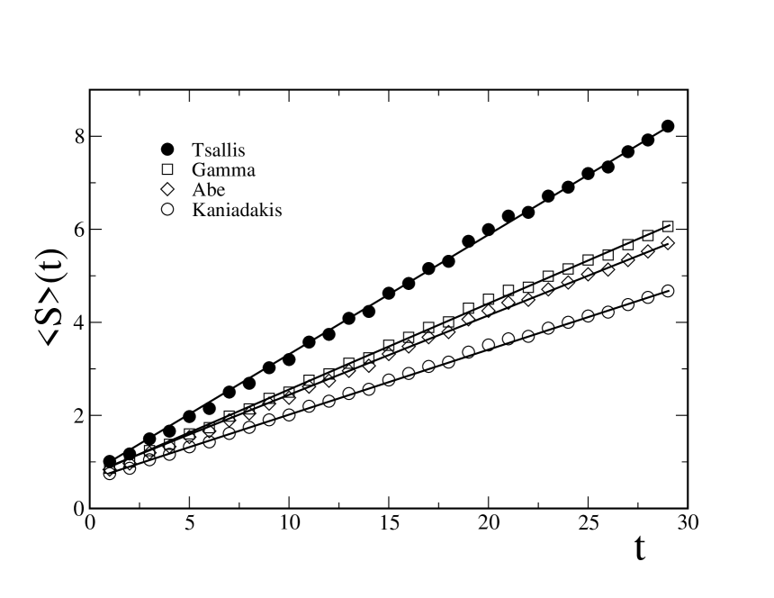
Figure 2: Entropy as function of time, averaged over $2\times 10^{4}$ experiments, each one with an ensemble of $10^{6}$ points over a grid of $10^{5}$ boxes. The entropies belong to the class of Eq. (2) and are defined with exactly the same exponents $\alpha$ and $\beta$ used for the sensitivities; as in Fig. 1, the curves show Tsallis’, $\gamma$, Abe’s, and Kaniadakis’ entropies from top to bottom. Straight lines are guides to the eyes.

The resulting rate of growth of several entropies $K_{\beta}=S_{\beta}(t)/t$ are (1) $0.267\pm 0.003$, (2) $0.197.\pm 0.002$, (3) $0.186\pm 0.002$, and (4) $0.152\pm 0.002$, where the statistical errors have been again estimated by sub-sampling the experiments. While this rate $K$ depends on the choice of the entropy, the generalized Pesin-like identity holds for each given deformation:

$$K_{\beta}=\lambda_{\beta}\quad.$$ (3)

III Width of the transition region

Since we follow the system for a finite amount of time and the sensitivity and entropy at each time step has a finite error, we expect that the statistical description of the system using a generalized formulation is practically useful not only at the precise onset of chaos, but also for values of $\mu$ slightly larger (fully chaotic region) or smaller (periodic region). To estimate the width of the interval of $\mu$, we have repeated the two previous experiments (sensitivity and entropy) with nine values of $\mu$: four above and four below the onset of chaos.

In Fig. 3 we report our result for the sensitivity in the case of Tsallis’ formulation: analogous results have been found for the other formulations. These curves should be compared with the top curve in Fig. 1. It appears that for $t<30$ all systems with $1.400\lessapprox\mu\lessapprox 1.402$ can be described by the generalized formalism. This estimate is confirmed by the corresponding curves for the entropy in Fig. 4.

For longer times the window shrinks: at $t=80$ already values of $\mu$ different by $0.03\%$ from the critical values deviate from the power-law behavior (see Fig. 3).

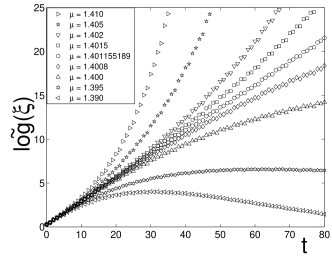
Figure 3: Generalized logarithms $\widetilde{\log}(\xi)$, see Eq. (1), of the sensitivity to initial conditions averaged over $10^{7}$ uniformly distributed initial conditions as function of time in the case of Tsallis’ formulation ($\beta=0$) for nine values of $\mu$. The central curve ($\mu=1.401155189$) is the top curve of Fig. 1; the four larger $\mu$ are in the chaotic region $\lambda>0$, the four smaller $\mu$ in the periodic one $\lambda<0$.

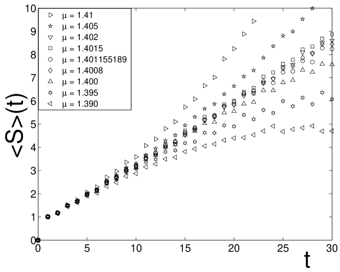
Figure 4: Tsallis’ entropy as function of time for the same nine values of $\mu$ of Fig. 3, averaged over $10^{4}$ experiments, each one with an ensemble of $10^{6}$ points over a grid of $10^{5}$ boxes.

IV Conclusions

In summary, numerical evidence corroborates and extends Tsallis’ conjecture that also weak chaotic systems can be described by an appropriate statistical formalism. Such extended formalisms should verify precise requirements (concavity, Lesche stability Kaniadakis:2004td ; Kaniadakis:2003ls ; Scarfone:2004ls , and finite-entropy production per unit time) to both correctly describe chaotic systems and provide a coherent statistical framework: the last criterion restricts the entropic forms to the ones with the correct asymptotic behavior. Using a specific two-parameter class that meets all these requirements, the logistic map shows:

(i) a power-low sensitivity to initial condition with a specific exponent $\xi\sim t^{1/\alpha}$, where $\alpha=0.650\pm 0.005$; this sensitivity can be described by deformed exponentials with the same asymptotic behavior $\xi(t)=\widetilde{\exp}(\lambda t)$ (see Fig. 1 for examples);

(ii) a constant asymptotic entropy production rate (see Fig. 2) for trace-form entropies with a specific power-behavior $p^{1-\alpha}$ in the limit of small probabilities only when the exponent $\alpha$ is the same appearing in the sensitivity;

(iii) a generalized Pesin-like identity holds $S_{\beta}/t\to K_{\beta}=\lambda_{\beta}$ for each choice of entropy and corresponding exponential in the class; the value of $K_{\beta}=\lambda_{\beta}$ depends on the specific entropy and it is not characteristic of the map.

We remark that the physical criterion of requiring that the entropy production rate reach a finite and non-zero asymptotic value has to consequences: (1) it selects a specific value of the parameter $\alpha$ ($\alpha$ is characteristic of the system); (2) strongly restricts the kind of acceptable entropies to the ones that have asymptotic power-law behavior (for instance it excludes Renyi entropy Johal:2004 ; Lissia:2005by ). The reason we ask for a finite non-zero slope is that otherwise we would miss an important characteristic of the system: its asymptotic exponent.

Finally we have estimated the range of $\mu$ for which the sensitivity to initial conditions and the entropy are well described by a power law behavior. The answer is clearly dependent on the maximum time considered and on our experimental resolution. For time smaller than 30 (80) the range appears of the order of 0.07 % (0.03%)

- (1) C. Tsallis, A. R. Plastino, and W.-M. Zheng, Chaos Solitons Fractals 8, 885 (1997).
- (2) R. Tonelli, G. Mezzorani, F. Meloni, M. Lissia and M. Coraddu, arXiv:cond-mat/0412730.
- (3) V. Latora and M. Baranger, Phys. Rev. Lett. 82, 520 (1999).
- (4) C. Tsallis, J. Statist. Phys. 52, 479 (1988).
- (5) M. Lissia, M. Coraddu and R. Tonelli, arXiv:cond-mat/0501299.
- (6) V. Latora, M. Baranger, A. Rapisarda and C. Tsallis, Phys. Lett. A 273, 97 (2000) [arXiv:cond-mat/9907412].
- (7) U. M.S. Costa, M. L. Lyra, A. R. Plastino and C. Tsallis, Phys. Rev. E 56, 245 (1997).
- (8) U. Tirnakli, G. F. J. Ananos and C. Tsallis, Phys. Lett. A 289, 51 (2001).
- (9) D.P. Mittal, Metrika 22, 35 (1975).
- (10) B.D. Sharma, and I.J. Taneja, Metrika 22, 205 (1975).
- (11) E.P. Borges, and I. Roditi, Phys. Lett. A 246, 399 (1998).
- (12) G. Kaniadakis and M. Lissia, Physica A 340, xv (2004) [arXiv:cond-mat/0409615].
- (13) G. Kaniadakis, M. Lissia, A. M. Scarfone, Physica A 340, 41 (2004) [arXiv:cond-mat/0402418].
- (14) G. Kaniadakis, M. Lissia, A. M. Scarfone, Phys. Rev. E 71, 046128 (2005) [arXiv:cond-mat/0409683].
- (15) J. Naudts, Physica A 316, 323 (2002) [arXiv:cond-mat/0203489].
- (16) F. Baldovin and A. Robledo, Phys. Rev. E 66, 045104(R) (2002) [arXiv:cond-mat/0205371].
- (17) F. Baldovin and A. Robledo, Europhys. Lett. 60, 518 (2002) [arXiv:cond-mat/0205356].
- (18) F. Baldovin and A. Robledo, Phys. Rev. E 69, 045202(R) (2004) [arXiv:cond-mat/0304410].
- (19) G. F. J. Ananos and C. Tsallis, Phys. Rev. Lett. 93, 020601 (2004) [arXiv:cond-mat/0401276].
- (20) S. Abe, Phys. Lett. A 224, 326 (1997).
- (21) G. Kaniadakis, Physica A 296, 405 (2001).
- (22) G. Kaniadakis, Phys. Rev. E 66, 056125 (2002) [arXiv:cond-mat/0210467].
- (23) G. Kaniadakis, Phys. Rev. E 72, 036108 (2005) [arXiv:cond-mat/0507311].
- (24) G. Kaniadakis and A.M. Scarfone, Physica A 340, 102 (2004) [arXiv:cond-mat/0310728].
- (25) S. Abe, G. Kaniadakis, and A.M. Scarfone, J. Phys. A (Math. Gen.) 37, 10513 (2004) [arXiv:cond-mat/0401290].
- (26) R. S. Johal and U. Tirnakli, Physica A 331, 487 (2004).