Energy fluctuations in vibrated and driven granular gases

Abstract

We investigate the behavior of energy fluctuations in several models of granular gases maintained in a non-equilibrium steady state. In the case of a gas heated from a boundary, the inhomogeneities of the system play a predominant role. Interpreting the total kinetic energy as a sum of independent but not identically distributed random variables, it is possible to compute the probability density function (pdf) of the total energy. Neglecting correlations and using the analytical expression for the inhomogeneous temperature profile obtained from the granular hydrodynamic equations, we recover results which have been previously observed numerically and which had been attributed to the presence of correlations. In order to separate the effects of spatial inhomogeneities from those ascribable to velocity correlations, we have also considered two models of homogeneously thermostated gases: in this framework it is possible to reveal the presence of non-trivial effects due to velocity correlations between particles. Such correlations stem from the inelasticity of collisions. Moreover, the observation that the pdf of the total energy tends to a Gaussian in the large system limit, suggests that they are also due to the finite size of the system.

1 Introduction

In non-equilibrium statistical mechanics the emergence of non-Gaussian distributions is a remarkable feature that marks an essential difference with typical results of equilibrium statistical mechanics. In particular, non-Gaussian behaviors for global quantities (i.e. system averaged) have been observed in different fields of physics racz03 , unveiling unexpected analogies between turbulent flows, equilibrium critical phenomena bramwell98 , and non-equilibrium instabilities brey05 . Averaged quantities are expected to be free of the microscopic details of the system under study, in such a way that their probability distribution function (pdf) should only depend on few parameters. Furthermore, they will contain relevant informations about the correlations among different parts of the system.

Granular gases represent a simple example of many-particles system out of equilibrium. The simplest model consists in an assembly of smooth hard particles undergoing binary inelastic collisions. This model, known as the Inelastic Hard Spheres (IHS) model, has stimulated a great interest for more than ten years. Its close similarity with the elastic hard spheres fluid has made possible the exploitation of the long-past known standard methods of kinetic theory. However the inclusion of energy dissipation in the collision law is sufficient to generate many surprising features that have been observed both in experiments and simulations, such as clustering, convection, non-equipartition of energy, etc. barrat05 ; poschel01 ; poschel03 .

In this paper we study the pdfs of the total kinetic energy of granular gases maintained in a non-equilibrium steady state by an external driving mechanism which compensates for the energy loss due to collisions. We first focus on boundary driven gases, since this kind of driving mechanism can easily be achieved experimentally, vibrating at high frequencies the container of the gas or one of its walls losert99b ; rouyer00 ; kudrolli00 ; wildman02 . Energy is hence provided at the boundaries and dissipated by inelastic collisions in the bulk of the system, leading to strong spatial inhomogeneities. A coarse-grained description of this steady state, in terms of density and temperature profiles, can be obtained by means of hydrodynamic equations brey00c , which are a priori valid when the mean-free-path is small compared to the typical length scale of the gradients. The presence of non-uniform density and temperature profiles implies that the total energy is a sum of variables which are not identically distributed and, in principle, correlated. We will first investigate the consequences of the lack of homogeneity by assuming total independence among the velocities, i.e. absence of correlations. Interestingly enough, this approximate approach leads to good estimates for the shape of the pdfs. Similarly, Bertin in a recent paper bertin05 showed that considering the sum of independent, but not identically distributed, random variables can be a useful way to explain (at least on a qualitative level) the emergence of non-Gaussian pdfs in other systems.

We will also discuss another important characteristic of such inhomogeneous systems, i.e. the fact that they are often non-extensive. Since the energy is injected from the boundaries and the dissipation happens inside the volume, it is clear that increasing the volume at constant density will not a priori increase the total energy linearly with the total number of particles $N$. The hydrodynamic approach allows to show that the relevant variable is the number of layers of particles at rest brey00c .

In order to disentangle the effects of inhomogeneities from those of correlations, we focus, in the second part of the paper, on the energy fluctuations in homogeneous granular gases. We will enforce homogeneity by considering the system in a pure velocity space, i.e. eliminating any spatial degree of freedom. When inhomogeneities disappear, the effects that may contribute, in the thermodynamic limit, to a non-Gaussian pdf of the total energy are the correlations among velocities. Nonetheless such a behavior generally shows up when the system is near some critical point, i.e. when some correlation length (in velocity space) diverges. A general theory for correlation functions for the hard sphere fluid has been first derived in ernst81 , and fruitfully applied to the homogeneous cooling state (HCS) for a gas of inelastic hard spheres brey04a . This last result was obtained exploiting the fact that the dynamics is dominated by the hydrodynamic (i.e. slow) modes, which are exactly computable for the particular case of the HCS. In our homogeneous models the total (kinetic) energy is the sum of $N$ identically distributed random variables. We will show, by numerical simulations, that in this state the central limit theorem applies and the energy pdf is a Gaussian in the large $N$ limit, which means that the correlation length in the velocity space is finite. The interesting issue then concerns the computation of the variance of the rescaled pdf. This quantity depends on the one-particle and (with a pre-factor $1/N$) two-particles distribution functions. It is deeply related to the finite size correlations between the velocities of the particles. In both cases of a stochastic and of a deterministic thermostat, its measure reveals the presence of non-trivial correlations. Remarkably, it only depends upon the restitution coefficient, but not upon other parameters such as the number of particles or the amplitude of the thermostating force. In the deterministic thermostated case, it is moreover in almost perfect agreement with the theoretical computations given in brey04a for a gas of inelastic hard spheres.

The structure of the paper is the following: in section II we discuss the gas driven at the boundaries, while in section III we consider the homogeneous thermostats. Conclusions are drawn in section IV.

2 The inhomogeneous boundary driven gas

The focus is here on the energy fluctuations of a granular gas in the case where energy is injected through a boundary, typically a vibrating wall. This kind of system corresponds to a realistic experimental setup losert99b ; rouyer00 ; kudrolli00 ; wildman02 and has therefore been widely studied both numerically and analytically grossman97 ; mcnamara97 ; mcnamara98b ; kumaran98 ; brey00c ; barrat02b . As an important consequence of the boundary heating, the density and the temperature are not homogeneous: a heat flux is present, which does not verify the Fourier law. This feature is well described by kinetic theory and in good agreement with the hydrodynamic approximation, which allows an analytical calculation of the density and temperature profiles brey00c . Recently Aumaître et al. aumaitre04 investigated, by means of Molecular Dynamics (MD), the fluctuations of the total energy of the system. In particular they have studied the behavior of the first two moments of the energy probability distribution function (pdf) when the system size is changed, at constant averaged density. Because of the inhomogeneities, the mean kinetic energy is no more proportional to the number of particles, and thus it is not an extensive quantity; analogously the mean kinetic temperature, defined as the average kinetic energy per particle, is no more intensive. This has led aumaitre04 to the proposal of a definition of an effective temperature $T_{E}$ and an effective number of particles $N_{f}$, such that $T_{E}$ is intensive and the total mean energy $\langle E\rangle=N_{f}T_{E}$ is extensive in this effective number of particles. In the following we will show how an approximate calculation which neglects correlations and the small non-Gaussianities, using the hydrodynamic prediction of brey00c for the temperature profile, allows in fact to explain the phenomenology observed in aumaitre04 . Within this description it is possible to obtain an explicit expression of the effective temperature and effective number of particles as a function of the system parameters (i.e. number of particles, restitution coefficient, and temperature of the vibrating wall). At large enough system sizes, the effective temperature is shown to be independent of the system size, while the effective number of particles is proportional to the surface of the heating boundary.

2.1 Energy Probability Distribution Function

We consider a granular gas of $N$ smooth inelastic hard spheres of diameter $\sigma$ between two parallel walls. The distance between the two walls is denoted by $H$, oriented along the $x$ axis. The linear extension of the wall is denoted by $L$, and periodic boundary conditions are applied along the directions parallel to the wall. One of the walls (in $x=0$) is vibrated, in order to compensate for the energy lost through inelastic collisions. As usual in the IHS model, the total momentum is conserved in collisions, and only the normal component of the velocity is affected. Thus, the collision law for a pair of particles $(1,2)$ reads:

$$\begin{cases}{\bf v}_{1}^{*}={\bf v}_{1}-\frac{1}{2}(1+\alpha)({\bf v}_{12}\cdot{\hat{\boldsymbol{\sigma}}}){\hat{\boldsymbol{\sigma}}}\\ {\bf v}_{2}^{*}={\bf v}_{2}+\frac{1}{2}(1+\alpha)({\bf v}_{12}\cdot{\hat{\boldsymbol{\sigma}}}){\hat{\boldsymbol{\sigma}}}\,\,,\\ \end{cases}$$ (1)

where $\hat{\boldsymbol{\sigma}}$ is a unitary vector along the center of the colliding particles at contact. In the dilute limit, such a system is well described by the Boltzmann equation, involving the one-particle distribution function $f({\bf r},{\bf v},t)$:

$$\partial_{t}f({\bf r},{\bf v}_{1},t)+{\bf v}\cdot{\boldsymbol{\nabla}}f({\bf r},{\bf v}_{1},t)=J[f|f]\,\,.$$ (2)

Here $J[f|f]$ is the collision integral, which takes into account the inelasticity of the particles:

$$J[f|f]=\sigma^{d-1}\int\textrm{d}{\bf v}_{2}\int_{{\bf v}_{12}\cdot\hat{\boldsymbol{\sigma}}>0}\textrm{d}\hat{\boldsymbol{\sigma}}({\bf v}_{12}\cdot\hat{\boldsymbol{\sigma}})\left(\frac{f({\bf r},{\bf v}_{1}^{**},t)f({\bf r},{\bf v}_{2}^{**},t)}{\alpha^{2}}-f({\bf r},{\bf v}_{1},t)f({\bf r},{\bf v}_{2},t)\right)\,\,,$$ (3)

where a collision transforms the couple (${\bf v}^{**}_{i},{\bf v}_{j}^{**})$ into $({\bf v}_{i},{\bf v}_{j})$. The hydrodynamic fields (local density $n$, local average velocity field ${\bf u}$, local temperature $T$) are defined as the velocity moments:

$$n({\bf r},t) =\int\textrm{d}{\bf v}f({\bf r},{\bf v},t)\,,$$ (4a)

$$n({\bf r},t){\bf u}({\bf r},t) =\int\textrm{d}{\bf v}\,{\bf v}f({\bf r},{\bf v},t)\,,$$ (4b)

$$\frac{d}{2}n({\bf r},t)T({\bf r},t) =\int\textrm{d}{\bf v}\frac{m}{2}({\bf v}-{\bf u})^{2}f({\bf r},{\bf v},t)\,,$$ (4c)

where $d$ is the space dimension. The hydrodynamic balance equations for the afore-defined fields are derived taking the velocity moments in (2). Then, it is possible to show that a steady state solution without macroscopic velocity flow exists: this solution is invariant for translations along all directions perpendicular to $x$, so that the hydrodynamic fields only depend upon $x$. Moreover this solution is stable if the size (in the directions perpendicular to $x$) of the system is smaller than a critical size which depends upon $\alpha$. In the rest of this section we consider such a “horizontally homogeneous” solution, whose temperature profile reads brey00c :

$$T(\ell)=T_{0}\left(\frac{\cosh{\left(\sqrt{a(\alpha)}(\ell_{m}-\ell)\right)}}{\cosh{\left(\sqrt{a(\alpha)}\ell_{m}\right)}}\right)^{2}\,\,,$$ (5)

where $a(\alpha)$ is a function of the restitution coefficient (its complete expression is given in ref. brey00c ). The variable $\ell$ is proportional to the integrated density of the system over the $x$ axis. Its definition is given by the following relation involving the local mean-free-path $\lambda(x)$:

$$\textrm{d}\ell=\frac{\textrm{d}x}{\lambda(x)}\,\,,\;\;\;\;\;\;\lambda(x)=\left[\frac{\sqrt{2}\pi^{\frac{d-1}{2}}}{{\Gamma[(d+1)/2]}}\sigma^{d-1}n(x)\right]^{-1}\,\,,$$ (6)

with $\ell=0$ at $x=0$. On the other hand, $\ell_{m}$ is the maximal $\ell$-value, reached at $x=H$:

$$\ell_{m}=C\sigma^{d-1}\,\int_{0}^{H}\textrm{d}x\,\,n(x)=C\sigma^{d-1}N_{x}\,\,,$$ (7)

where $N_{x}$ is the number of particles per unit section perpendicular to the $x$ axis (e.g. $N_{x}=N/L$ for $d=2$), and $C$ is a constant depending on the dimension (e.g. $C=2\sqrt{2}$ for $d=2$). It thus turns out that the crucial quantity $\ell_{m}$ which determines the hydrodynamic profiles is proportional to the number of layers of particles at rest. The boundary conditions used to get expression (5) are:

$$T(\ell=0)=T_{0}\,\,,\,\,\,\,\,\,\,\,\,\,\left.\frac{\partial T}{\partial\ell}\right|_{\ell=\ell_{m}}=\,\,\left.\frac{\partial T}{\partial x}\right|_{x=H}=0\,\,,$$ (8)

where we have assumed that the vibrating wall acts as a thermostat that fixes to $T_{0}$ the temperature at $x=0$. A detailed observation would show that this is not a very realistic assumption. Moreover, the region in the vicinity of $x\sim 0$ is the one in which the hydrodynamic description may break down. Nevertheless, $T_{0}$ may be seen as an effective parameter such that (5) coincides with the observed profile in the region of the system where hydrodynamics holds. In the following we will suppose the velocity distribution to be a Maxwellian at each fixed distance from the wall (non-Gaussian features may be observed, but are not relevant for the present calculation), with a local temperature (variance) given by (5):

$$f({\bf v},\ell)={e^{-{v^{2}\over 2T(\ell)}}\over\sqrt{2\pi T(\ell)}}\,\,.$$ (9)

The distribution for the energy of one particle ($e=v^{2}/2$) is hence:

$$p(e,\ell)=f_{{1\over T(\ell)},{d\over 2}}(e)\,\,\,,$$ (10)

where $f_{\alpha,\nu}(x)$ is the gamma distribution feller :

$$f_{\alpha,\nu}(x)={\alpha^{\nu}\over\Gamma(\nu)}x^{\nu-1}e^{-\alpha x}\,.$$ (11)

The characteristic function of the gamma distribution is:

$${\tilde{f}}_{\alpha,\nu}(k)=\int_{-\infty}^{+\infty}\textrm{d}xe^{\textrm{i}kx}f_{\alpha,\nu}(x)=\left(1-\frac{\textrm{i}k}{\alpha}\right)^{-\nu}\,\,.$$ (12)

Our interest goes to the macroscopic fluctuations integrated over all the system. Thus, the macroscopic variable of interest is the granular temperature $T_{g}$, defined here as the average of the local temperature over the $x$ profile:

$$T_{g}={1\over N}\int_{V}n({\bf r})T({\bf r})\,\,\textrm{d}{\bf r}={1\over\ell_{m}}\int_{0}^{\ell_{m}}T(\ell)\,\,\textrm{d}\ell\,\,.$$ (13)

To obtain an expression of the energy pdf over all the system, it is useful to divide the box in $\ell_{m}/\Delta\ell$ boxes of equal height (in the $\ell$ scale) $\Delta\ell$. The use of this length scale allows to have a fixed number of particle $N_{\ell}$ in each box of size $L\times\Delta\ell$, since $d\ell\propto n(x)dx$. Moreover, in each box $i$ the temperature can be taken as uniform, denoted $T_{i}\equiv T(i\,\,\Delta\ell)$. In the $j-th$ box, we can calculate the energy $\epsilon_{j}$ which is the sum of the energies of the $N_{\ell}$ particles in the box. The pdf of this energy, $q_{j}(x)=\textrm{prob}(\epsilon_{j}=x)$, can be straightforwardly computed when the velocities of the particles are supposed to be uncorrelated:

$$q_{j}(x)=f_{{1\over T_{j}},N_{\ell}\frac{d}{2}}(x)\,\,\,,$$ (14)

Thus, the characteristic function for the total kinetic energy $E=\sum\epsilon_{j}$ can be obtained as the product of the characteristic function ${\tilde{q}}_{j}(k)$ of the pdf of each $\epsilon_{j}$:

$${\widetilde{P}}(k)=\prod_{j=0}^{\ell_{m}/\Delta\ell}{\tilde{q}}_{j}(k)=\prod_{j=0}^{\ell_{m}/\Delta\ell}(1-\textrm{i}kT_{j})^{-\frac{N_{\ell}d}{2}}\,\,\,.$$ (15)

Since the number of particle per box $N_{\ell}$ is a known fraction of the total number of particles ($N_{\ell}=N\Delta\ell/\ell_{m}$), one can rewrite the expression (15) as a Riemann sum. In the limit $\Delta\ell\to 0$ this yields the total kinetic energy characteristic function:

$${\widetilde{P}}(k)=\exp\left(\,-{Nd\over 2\ell_{m}}\int_{0}^{\ell_{m}}\log\left(1-\textrm{i}kT(\ell)\right)\,\,\textrm{d}\ell\right)\,\,.$$ (16)

Note that this result is valid for any temperature profile $T(\ell)$ and hence it can be applied also to other situations with different boundary conditions or different hydrodynamic equations.

2.2 Local energy fluctuations

While we have focused on the pdf of the global energy in the previous subsection, it is also interesting to consider an intermediate scale and to compute the energy pdf for a ”slice” of the system at a given distance $x$ from the vibrating wall, and of small height $\Delta x$ (such that the local density and temperature can be considered as uniform). We still consider that the velocities are Gaussian and uncorrelated. In this case the energy $\epsilon$ is a sum of $N(x)$ identically distributed random variables, but their number $N(x)$ fluctuates in time. Hence the pdf of the local energy is:

$$P_{l}(\epsilon,x)=\sum_{N(x)=1}^{\infty}P_{d}(N(x))f_{\frac{1}{T(x)},N(x)\frac{d}{2}}(\epsilon)+P_{d}(0)\delta(\epsilon)\,\,,$$ (17)

where $P_{d}$ is the distribution of the number of particles at a distance $x$ from the heated wall. The second term in the above expression is due to the fact that when there are no particles the energy pdf is a Dirac distribution. If the particles are uncorrelated the distribution $P_{d}$ should be well approximated by a Poisson distribution with average $\langle N(x)\rangle=n(x)\Delta x$:

$$P_{d}(N(x)=i)=e^{-n(x)\Delta x}\frac{(n(x)\Delta x)^{i}}{i!}\,\,.$$ (18)

In this framework the explicit expression for the probability of the local energy is given, in two dimensions, by:

$$P_{l}(\epsilon,x)=e^{-n(x)\Delta x-\frac{\epsilon}{T(x)}}\ \sqrt{\frac{n(x)\Delta x}{T(x)\epsilon}}\,I_{1}\left(2\sqrt{\frac{n(x)\Delta x\ \epsilon}{T(x)}}\right)+2e^{-n(x)\Delta x}\delta(\epsilon)\,\,,$$ (19)

where $I_{n}(x)$ is the first kind modified Bessel function abramowitz . For higher dimensions the sum in Eq. (17) with Poissonian density fluctuations can be expressed as a combination of generalized hypergeometric functions. The cumulants of those distributions are, in general dimension $d$:

$$\langle\epsilon^{p}\rangle_{c}(x)=\frac{n(x)\Delta xT^{p}(x)}{2^{p}}d(d+2)\dots(d+2p-2)\,\,,$$ (20)

where the notation $\langle X\rangle_{c}$ denotes the cumulant of the variable $X$.

2.3 Comparison with simulations

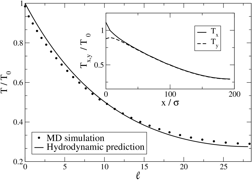
Figure 1: Temperature profile in the $\ell$ scale for a system of $N=1000$ particles in a box of height $H=200\,\sigma$ and density $n\sigma^{2}=0.05$ with $\alpha=0.99$. The temperature is scaled with the temperature near the vibrating wall $T_{0}$. The inset show the temperature profile of the $x$ and $y$ component in the $x$ scale, showing that the temperature is effectively isotropic apart from a small region near the vibrating wall.

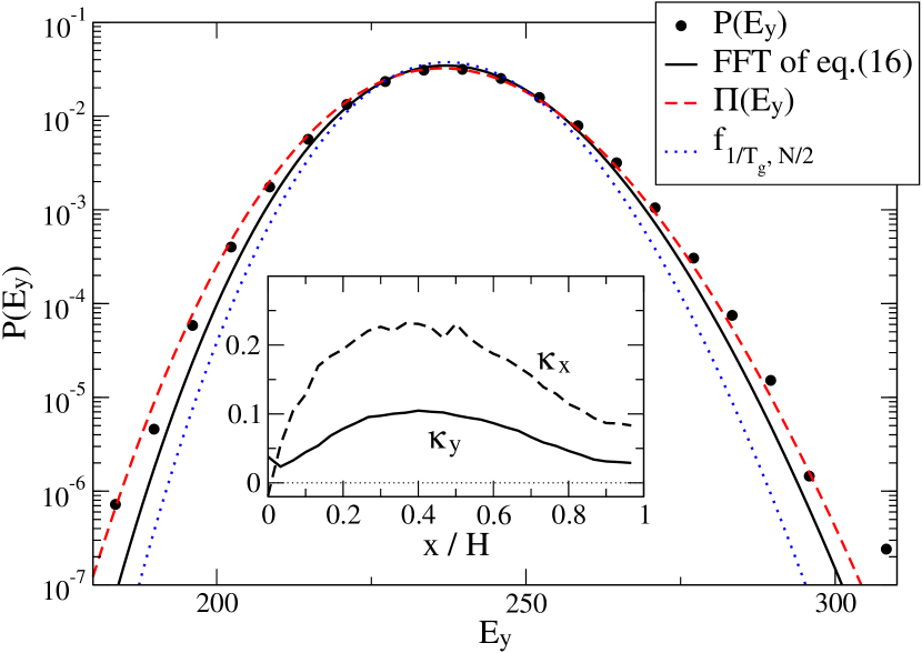
Figure 2: Probability density function of the $y$ component of the total energy $E_{y}=\sum_{i}^{N}v_{y_{i}}^{2}$ (dots). The parameters of the system are the same as in Fig. 2. The solid line is the numerical inverse Fourier transform of Eq. (16), while the dashed line is a $\chi^{2}$ distribution with same mean and same variance of the numerical data, and the dotted line a $\chi^{2}$ distribution with parameters corresponding to the granular temperature and the true number of degrees of freedom. The energy is in units of the temperature of the wall $T_{0}$. The inset shows the kurtosis excess $\kappa_{i}=\langle v_{i}^{4}\rangle/\langle v_{i}^{2}\rangle^{2}-3$ for the $x$ and $y$ component of the velocity pdf.

To obtain the analytic form of the energy pdf one should calculate the inverse Fourier Transform of equation (16) using (5) as temperature profile. This does not seem possible analytically, but one can resort to numerical procedures. Aumaître et al. aumaitre00a ; aumaitre04 have shown by Molecular dynamic simulations that the energy pdf is very well fitted by a $\chi^{2}$ law, but with a number of degrees of freedom different from $N\,d$, and a temperature different from the granular temperature $T_{g}$. They proposed to define an effective number of degrees of freedom $N_{f}$ and an effective temperature $T_{E}$, such that energy pdf should be of the form $\Pi(E)=f_{{1\over T_{E}},{N_{f}\over 2}}(E)$, with:

$$N_{f}=2\,{\langle E\rangle_{c}^{2}\over{\langle E^{2}\rangle_{c}}}\,,\;\;\;\;\;\;\;\;\;\;\;\;\;\;\;\;\;\;\;\;T_{E}={\langle E^{2}\rangle_{c}\over\langle E\rangle_{c}}\,\,.$$ (21)

In Fig. 2 a direct comparison between the measured temperature profile in the $\ell$-scale and the theoretical prediction of Eq. (5) shows the agreement between the Molecular Dynamics (MD) simulation and the hydrodynamic prediction. In Fig. 2, the Inverse Fourier Transform of (16) is compared with the pdf of the $y$ component of the total energy obtained from MD simulations, showing a good agreement. We restrict our analysis to the $y$ component because the velocity pdf in this direction is closer to the Gaussian distribution (as quantified in the inset by the excess kurtosis, see also brey00c ), and is therefore in better agreement with our hypotheses. In the same figure we have also plotted the function $\Pi(E)$ previously defined, which has a similar shape and yields a better fit of the numerical data. We emphasize however that our prediction needs only one fitting parameter, $T_{0}$, which essentially fixes the average of the distribution, while in order to have a closed form for $\Pi(E)$ one needs to know both the mean and the variance of the distribution. This underlines the importance of the inhomogeneous hydrodynamic profile in determining the fluctuations of the global energy; on the other hand, the correlations, which have been neglected in our approximate approach, seem to play a lesser role.

Our approach also allows to investigate the behavior of the macroscopic quantities $N_{f}$ and $T_{E}$ when the system size is changed. Indeed, an expression of the cumulants of the total kinetic energy can be obtained from the characteristic function (16):

$$\langle E^{p}\rangle_{c}={Nd\over 2\ell_{m}}\int_{0}^{\ell_{m}}T^{p}(\ell)\textrm{d}\ell\,\,\,,$$ (22)

so that

$$N_{f}=\frac{Nd}{\ell_{m}}\frac{\left(\int_{0}^{\ell_{m}}T(\ell)d\ell\right)^{2}}{\int_{0}^{\ell_{m}}T^{2}(\ell)d\ell}\,,\;\;\;\;\;T_{E}=\frac{\int_{0}^{\ell_{m}}T^{2}(\ell)d\ell}{\int_{0}^{\ell_{m}}T(\ell)d\ell}\ ,$$ (23)

which shows that $T_{E}$ is not rigorously intensive but depends on the number of layers of particles through $\ell_{m}$. At large enough $\ell_{m}$ however, the integral in equation (22) becomes size independent:

$$\int_{0}^{\ell_{m}}T^{p}(\ell)\textrm{d}\ell\sim{T_{0}^{p}\over 2p\sqrt{a(\alpha)}}\,\,,$$ (24)

so that the effective temperature $T_{E}$ defined above becomes a constant proportional to the temperature of the wall, while the parameter $N_{f}$ still depends on the system size:

$$N_{f}\sim{1\over\sqrt{a(\alpha)}}\,{Nd\over\ell_{m}}\,,\;\;\;\;\;\;\;\;\;\;\;\;\;\;\;\;\;\;\;\;T_{E}\sim{T_{0}\over 2}.$$ (25)

We now investigate how the numerical results of aumaitre04 fit with the previous framework, for the various possibilities of system size variations at fixed particle size $\sigma$ and constant density $\rho=N/(HL)$ (we consider for simplicity a two-dimensional system, as in aumaitre04 ):

• if only $L$ is increased, at constant $H$, $N/L$ is constant so that $\ell_{m}$ and thus $T_{E}$ do not change

• if only $H$ is increased, at constant $L$, $\ell_{m}\propto N/L$ increases so that $T_{E}$ is not constant. The variation of $T_{E}$ with $H$ is however slow and moreover, as soon as $N$ is large enough, $T_{E}$ reaches its asymptotic value $T_{0}/2$.

• if both $H$ and $L$ are increased at the same rate, $\ell_{m}$ increases slower so that once again $T_{E}$ is not rigorously constant but varies slowly towards $T_{0}/2$.

The behavior of $N_{f}$ also depends on the maximum of the integrated density $\ell_{m}$. At constant $\sigma$ and density $\rho=N/(HL)$, Eq. (25) shows that (i) for a square cell, since $\ell_{m}\propto\sqrt{N}$ , one obtains $N_{f}\propto\sqrt{N}$, close to the $N^{0.4}$ behavior numerically observed in aumaitre04 , and (ii) at constant $L$, if only the height $H$ of the cell is increased, $\ell_{m}$ is proportional to $N$, and $N_{f}$ thus becomes constant. All these features are in agreement with the numerical observations in aumaitre04 . The above results show that the issues of intensivity and extensivity can be understood through an approximate approach which neglects correlations but focuses on the inhomogeneities as described by the hydrodynamic profiles brey00c . The crucial quantity turns out to be the number of layers of particles at rest. If this number is large enough, the effective temperature $T_{E}$ becomes intensive. Moreover, this approach is able to quantitatively describe the behavior of the fluctuations of the total kinetic energy of a vibrated granular gas. In some cases the energy pdf can be approximated with a gamma distribution, which is the standard distribution for the energy pdf in the canonical equilibrium. Nevertheless there are strong deviations from the equilibrium theory of fluctuations, since in this case the two parameters of the gamma distribution (i.e. the temperature and the number of degrees of freedom) are not the granular temperature nor the total number of degrees of freedom. Another important remark is that correlations, and in particular contributions from the two points distribution function, do not play a primary role in explaining those deviations from the equilibrium theory of fluctuations. In order to characterize deviations which do not arise from inhomogeneities, it can be useful to measure energy fluctuations at a given height $x$ from the vibrating wall. From the expression of the cumulants of the local energy pdf (20) it is possible to define an “effective density” (of particles) $n_{f}(x)=\frac{d(d+2)}{d^{2}}\frac{\langle\epsilon\rangle^{2}}{\langle\epsilon^{2}\rangle_{c}}$. If the uncorrelated and Gaussian hypotheses are satisfied, then $n_{f}(x)=n(x)$, and deviations from this identity should be due only to correlations and non-Gaussianities. In Figs. 4 and 4 results from MD simulations are shown at various values of the inelasticity, density and number of particles. The agreement between Eq. (19) and the numerical data is very good, while the deviations from $n_{f}(x)=n(x)$ shown in Fig. 4, are evident but small compared to the deviations between $N_{f}$ and $N$.

Another way to discriminate the respective role of heterogeneities and of correlations for the global system is to study granular gases maintained in an homogeneous state by a suitable energy injection, as proposed below.

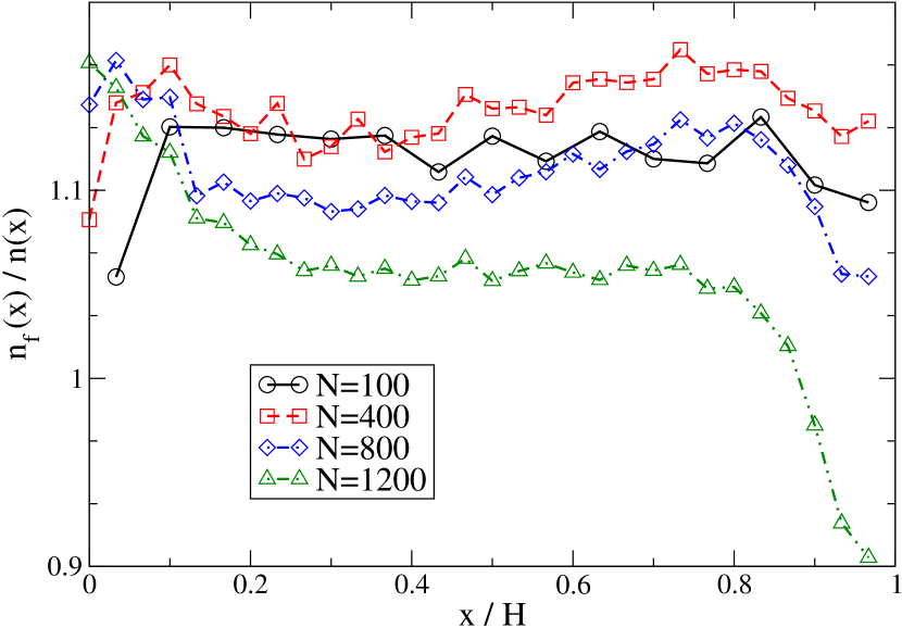
Figure 3: Plot of the effective density $n_{f}(x)$ divided by the true density $n(x)$ in a square box at constant density $\rho\sigma^{2}=0.04$ for $\alpha=0.99$ and several system sizes. The corresponding effective numbers of degrees of freedom are, when the number of particles and the volume are increased at constant density: $N_{f}/(Nd)=0.99$; $N_{f}/(Nd)=0.77$; $N_{f}/(Nd)=0.63$; $N_{f}/(Nd)=0.47$.

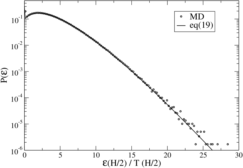
Figure 4: Plot of the local energy pdf for a system of $N=100$ particles in a square cell at density $\rho\sigma^{2}=0.04$ and $\alpha=0.95$. The energy has been sampled in a strip of width $\Delta x=1.66\,\sigma$ centered in $x=H/2$. The solid line is the analytical estimation from Eq. (19).

3 The homogeneously driven case

In this section we consider a granular gas kept in a stationary state by an external homogeneous thermostat. Two different kinds of thermostat will be used. We will first consider the so called “Stochastic thermostat”, which is a white noise acting independently on each particle williams96b ; noije98c ; puglisi99 ; noije99 ; montanero00b ; moon01 ; garzo02b . In a second part we will show some numerical results concerning the “Gaussian thermostat”, which consists of a negative friction force acting on each particle montanero00b ; garzo02b .

3.1 Stochastic thermostat

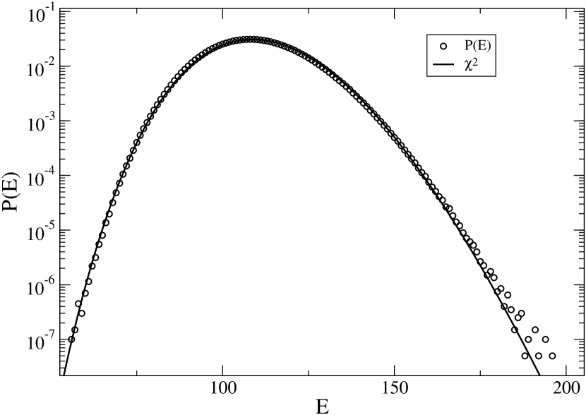
Figure 5: Energy pdf (dots) from DSMC simulations with a restitution coefficient $\alpha=0.5$ and $N=100$ particles for a system driven with the stochastic thermostat. The solid line shows a gamma distribution with same mean and same variance.

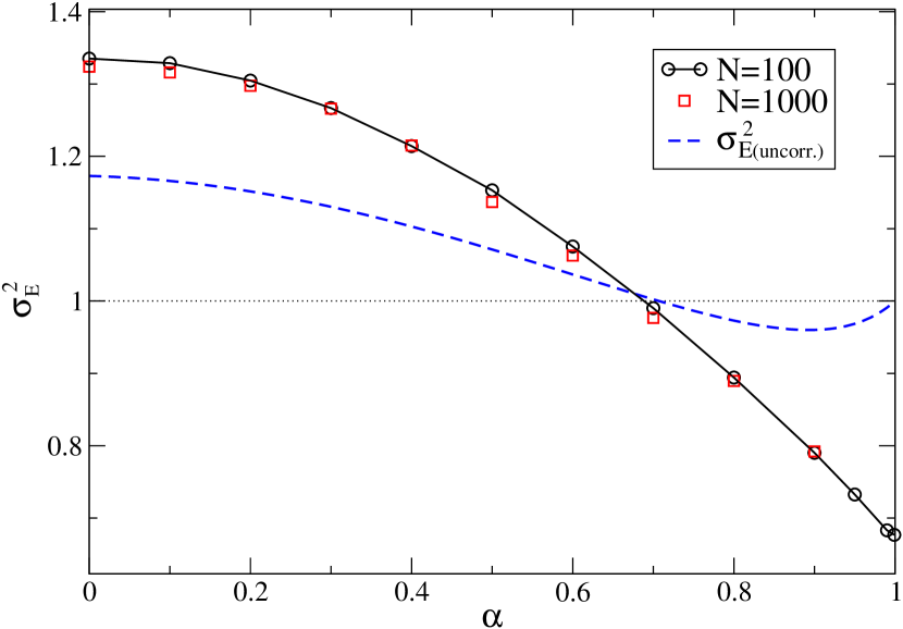
Figure 6: Plot of $\sigma^{2}_{E}$ versus the restitution coefficient $\alpha$ for $N=100$ ($\bigcirc$) and $N=1000$ ($\square$) particles driven by the stochastic thermostat. The result of the calculation assuming uncorrelated velocities (37) is plotted in dashed line.

We consider here a gas of $N$ inelastic smooth hard spheres driven by an external random noise. The equation of motion of each particle $i$ is:

$${\textrm{d}{\bf v}_{i}\over\textrm{d}t}={{\bf F}^{c}_{i}\over m}+\hat{{\boldsymbol{\xi}}}_{i}(t)\,,$$ (26)

where ${\bf F}^{c}_{i}$ is the force due to inelastic collisions [the latter being ruled by Eqs. (1)], and $\hat{{\boldsymbol{\xi}}}_{i}$ is the random acceleration due to the stochastic force, which is assumed to be an uncorrelated Gaussian white noise:

$$\langle{\hat{\xi}}_{i\alpha}(t){\hat{\xi}}_{j\beta}(t^{\prime})\rangle=\xi_{0}^{2}\delta_{ij}\delta_{\alpha\beta}\delta(t-t^{\prime})\,\,,$$ (27)

where $i$ and $j$ denote the labels of the particles, while $\alpha$ and $\beta$ refer to the Euclidean component of the noise. Our interest goes to the stationary state of such system, which is homogeneous, and furthermore does not develop spatial instabilities. A good description of such a system can therefore be obtained through a homogeneous Boltzmann equation, which will contain a Fokker-Planck diffusion term, taking into account the stochastic force. This equation reads noije98c :

$$\partial_{t}f({\bf v}_{1},t)=J[f|f]+{\xi_{0}^{2}\over 2}\left({\partial\over\partial{\bf v}_{1}}\right)f({\bf v}_{1},t)\,\,,$$ (28)

where $J[f|f]$ is the collision integral (cf. Eq. 3). The stationary solution of this equation is well approximated by the product of a Gaussian with a Sonine Polynomial

$$f({\bf c})={e^{-c^{2}}\over\pi^{d/2}}(1+a_{2}S_{2}(c^{2}))\,\,,$$ (29)

where ${\bf c}={\bf v}/v_{0}$ is a dimensionless velocity, with $v_{0}=\sqrt{2T}$, $S_{2}(x)$ is the second Sonine polynomial

$$S_{2}(x)={1\over 2}x^{2}-{1\over 2}(d+2)x+{1\over 8}d(d+2)\,\,,$$ (30)

and $a_{2}$ is a coefficient proportional to the kurtosis of the function $f({\bf c})$:

$$a_{2}={4\over d(d+2)}\left[\langle c^{4}\rangle-{1\over 4}d(d+2)\right]={4\over 3}\left[\langle c_{x}^{4}\rangle-3\langle c_{x}^{2}\rangle^{2}\right]\,\,.$$ (31)

An approximate expression of the coefficient $a_{2}$ for an arbitrary restitution coefficient is noije98c :

$$a_{2}(\alpha)={16(1-\alpha)(1-2\alpha^{2})\over 73+56d-24\alpha d-105\alpha+30(1-\alpha)\alpha^{2}}\,\,.$$ (32)

The energy dissipated in the inelastic collisions is compensated by the energy injected by the thermostat so that the system reaches a stationary state, in which the temperature fluctuates around its mean value

$$T_{g}=m\left(\frac{d\xi_{0}^{2}\sqrt{\pi}}{(1-\alpha^{2})\Omega_{d}n\sigma^{d-1}}\right)^{2/3}(1+{\cal O}(a_{2}))\,\,,$$ (33)

where $\Omega_{d}$ is the $d$-dimensional solid angle, $m$ the mass of the particle, and $n$ the density of the system. Here we are interested in the fluctuations of the total energy measured by the quantity

$$\sigma_{E}^{2}=N{\langle E^{2}(t)\rangle-\langle E(t)\rangle^{2}\over\langle E(t)\rangle^{2}}\,\,.$$ (34)

Note that $\sigma_{E}^{2}\equiv 2N/N_{f}$, and that $T_{g}$ is intensive while the total energy is extensive. Brey et al. have computed, by means of kinetic equations, an analytical expression for $\sigma_{E}^{2}$ in the homogeneous cooling state, which is equivalent to the so-called Gaussian deterministic thermostat brey04a . This quantity has also been computed in a one dimensional granular gas with a similar thermostat cecconi2004 . One of the main differences of the stochastic thermostat with a deterministic one is found in the elastic limit. On the one hand, for the cooling state, when the restitution coefficient tends to $1$, the conservation of energy imposes that the energy pdf is a Dirac delta function, and the quantity $\sigma_{E}$ goes to $0$. On the other hand, with the stochastic thermostat, if the elastic limit is taken keeping the temperature constant, the strength of the white noise will tend to zero, but it will still play a role in the velocity correlation function (we note that it is not necessary to keep the temperature constant while performing the limit, since this quantity only sets an irrelevant time scale).

An efficient way to have numerical solutions of Boltzmann-like equations is the so called Direct Simulation Monte Carlo (DSMC). This algorithm simulates a Markov chain whose associated master equation is expected to converge to the Boltzmann equation. We performed this kind of simulation to measure the energy pdf. A plot of this quantity is shown in Fig. 6. We observe again that it is close to a $\chi^{2}$-distribution with same mean and same variance. Nevertheless the number of degrees of freedom of this $\chi^{2}$-distribution is lower than the true number of degrees of freedom (i.e. $(N-1)\times d$). This effect may arise from two separated causes: the non-gaussianity of the velocity pdf, and the presence of correlations between the velocities. This feature also suggests that a calculation of the energy pdf with the hypothesis of uncorrelated velocities (but non-Gaussian) could explain at least a part of this non-trivial effect. The calculation of the pdf of the sum of the square of $n$ variables distributed following (29) is straightforward. The characteristic function of the energy pdf is:

$${\widetilde{P}}_{N}(k)={1\over(1-\textrm{i}kT)^{Nd\over 2}}\left(1+{d(d+2)\over 8}a_{2}\left({1\over(1-\textrm{i}kT)^{2}}-{2\over(1-\textrm{i}kT)}+1\right)\right)^{N}$$ (35)

where $N$ is the number of particles of the system. This results yields

$$\langle E\rangle={d\over 2}NT\,\,,\;\;\;\;\langle E^{2}\rangle-\langle E\rangle^{2}={d\over 2}NT^{2}\left(1+{d+2\over 2}a_{2}\right)\,\,,$$ (36)

so that the explicit expression for the energy fluctuations reads:

$$\sigma^{2}_{E_{(uncorr.)}}={2\over d}\left(1+{d+2\over 2}a_{2}\right)\,\,.$$ (37)

As expected, the temperature does not appear in the dimensionless $\sigma_{E}^{2}$ above, which depends on the only available dimensionless parameters $\alpha$ and $d$. This result is compared in Fig. 6 with the result of DSMC simulations, carried out for several values of the restitution coefficient $\alpha$ and for two different values for the number of particles $N$. The disagreement between the uncorrelated calculation and the simulations is a clear sign of the correlations induced by the inelasticity of the system (the tail of the velocity pdf is also non-Gaussian noije98c , but this feature has negligible consequences for the quantities of interest here). One can note that the fluctuations increase when the restitution coefficient decreases. One can also see that there is a value of the restitution coefficient $\alpha$ around $1/\sqrt{2}$, that is when the approximate expression of $a_{2}$ vanishes, for which $\sigma_{E}^{2}$ is exactly $1\equiv 2/d$, as for a gas in the canonical equilibrium.

We now turn to the dependence of $\sigma^{2}_{E}$ on the strength of the white noise $\Gamma$. It is useful, for this purpose, to introduce a rescaled, dimensionless energy

$${\widetilde{E}}={E-\langle E\rangle\over\sqrt{\langle E^{2}\rangle-\langle E\rangle^{2}}}\,\,.$$ (38)

We have plotted in Fig. 8 this rescaled energy pdf for a system of $N=100$ particles with a restitution coefficient $\alpha=0.5$ and for several values of the strength of the white noise $\Gamma$. As expected, all the pdfs collapse into a unique distribution: the role of the noise’s strength is only to set the temperature (or mean kinetic energy) scale. Besides, relative energy fluctuations depend only on $\alpha$ and $N$. Moreover, since $\sigma_{E}^{2}$ does not depend on the number of particles $N$ (for $N$ large enough), $\sqrt{\langle E^{2}\rangle-\langle E\rangle^{2}}$ grows as $\sqrt{N}$, so that the central limit theorem applies, and hence $P({\tilde{E}})$ is a Gaussian in the thermodynamic ($N\to\infty$) limit. Figure 8 indeed shows how the rescaled energy pdf for $N=1000$ particles is very close to a Gaussian, even if the $\chi^{2}$-distribution still gives a better fit.

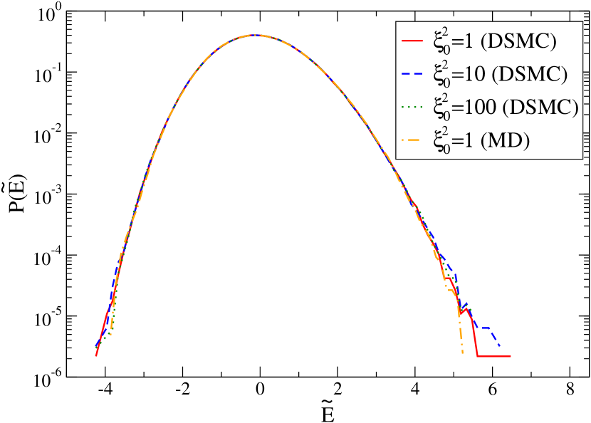
Figure 7: Plot of the pdf of ${\widetilde{E}}$ for a restitution coefficient $\alpha=0.5$, for $N=100$ particles, and for several values of the noise’s strength $\xi_{0}^{2}$. The simulations have been carried on with both Monte-Carlo (DSMC) and Molecular Dynamics (MD) algorithms, with $n\sigma^{2}=0.04$.

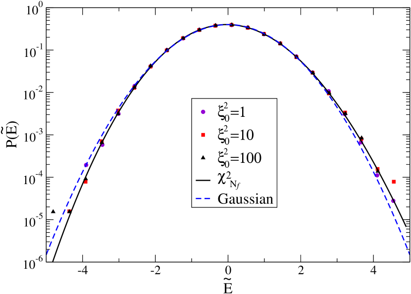
Figure 8: Plot of the pdf of ${\widetilde{E}}$ for a restitution coefficient $\alpha=0.5$, for $N=1000$ particles, and for several values of the noise’s strength $\xi_{0}^{2}$. The solid line is a rescaled $\chi^{2}$-distribution with $N_{f}=2N/\sigma_{E}^{2}\simeq 1759$ degrees of freedom, and it is very close to the Gaussian distribution, plotted here in dashed line.

3.2 Gaussian thermostat

In this section, we will focus on the fluctuations in a granular gas driven by a Gaussian thermostat , which consist in adding a viscous force, with a negative friction coefficient, in the equation of motion of each particle. Thus the velocity of the $i$-th particle will verify the following equation:

$$\frac{\textrm{d}{\bf v}_{i}}{\textrm{d}t}=\frac{{\bf F}^{c}_{i}}{m}+\gamma{\bf v}_{i}\,\,.$$ (39)

In the above equation ${\bf F}^{c}$ is the force due to collisions, and $\gamma$ is a positive constant. The Boltzmann equation corresponding to Eq. (39) is:

$$\partial_{t}f({\bf v}_{1},t)=J[f|f]-\gamma\frac{\partial}{\partial{\bf v}_{1}}\cdot[{\bf v}_{1}f({\bf v}_{1},t)]\,\,\,.$$ (40)

In this case also, the relevant solution is well approximated by a Gaussian multiplied with a Sonine polynomial [cf. Eq. (29)]. The expression of the coefficient $a_{2}$ has been widely studied noije98c ; montanero00b ; coppex03 , and the one which is in better agreement with numerical simulations is the following montanero00b :

$$a_{2}(\alpha)=\frac{16(1-\alpha^{2})(1-2\alpha^{2})}{25+24d-\alpha(57-8d)-2(1-\alpha)\alpha^{2}}\,\,.$$ (41)

The parameter $\gamma$ determines the strength of the homogeneous force acting on the particles. Its primary role is to set the temperature scale of the stationary state. Projecting Eq. (40) on the second velocity moment is it possible to get an approximate expression of the stationary temperature:

$$T\simeq m\left(\frac{2\sqrt{\pi}\gamma d}{(1-\alpha^{2})\Omega_{d}n\sigma^{d-1}}\right)^{2}(1+{\cal O}(a_{2}))\,\,.$$ (42)

This result has been obtained assuming Gaussian velocity pdf, since the corrections coming from the coefficient $a_{2}$ are small.

Equation (40) is formally equivalent to the Boltzmann equation for the homogeneous cooling state (HCS) of a granular gas, for the particular solution in which all the time dependence of the velocity pdf appears trough the time dependent temperature goldshtein95 . This mapping of the cooling state onto a steady state can be obtained in an equivalent fashion applying a logarithmic time-scale transformation to the time-dependent Boltzmann equation of the HCS lutsko01 ; brey04a . Furthermore, the above scaling solution can be extended to the $n$-particle distribution function of the system. The resulting hierarchy equations of the HCS are then exactly the same one would obtain for a homogeneous granular gas thermostated by a Gaussian thermostat. Thus these two models not only have the same velocity pdf, but also the same $n$-particles distribution, and hence they will have the same relative fluctuations and correlation functions. Henceforth we will no more make any distinction between the HCS and the Gaussian thermostat. We will therefore compare results obtained for the HCS with numerical simulations of a gas driven in a stationary state with a Gaussian thermostat. We also have to note that this kind of homogeneous state is unstable under small density fluctuations, and naturally develops cluster and shear instabilities. In the following we will therefore focus only on homogeneous states. For the HCS Brey et al. brey04a have obtained an analytical expression for the quantity $\sigma_{E}^{2}$ defined in Eq. (34). Its expression is:

$$\sigma_{E}^{2}=\frac{d(d+1)}{2}+\frac{d(d+2)}{4}a_{2}(\alpha)+d^{2}b(\alpha)\,\,,$$ (43)

where

$$b(\alpha)=\frac{4\,\left(1-2\,\alpha^{2}\right)\,\left(1-3\,\alpha+\alpha^{2}\,\left(\alpha-1\right)\right)-\left(1-\alpha\right)\,\left(3-2\,\alpha\,\left(8+5\,\alpha\right)\right)\,d-2\,\left(3+\alpha\right)\,d^{2}}{2\,d\,\left(7+6\,d-\alpha\,\left(15+2\,\alpha\left(1-\alpha\right)-2\,d\right)\right)}\,\,.$$ (44)

Note that $b(1)=-(1+d)/(2d)$ so that $\sigma_{E}^{2}\to 0$ as $\alpha\to 1$. The results from DSMC simulations and the theoretical predictions by Brey et al. are shown in Fig. 10. The simulations have been carried out for two different sizes of the system ($N=100$ and $N=1000$), and for several values of $\alpha$, and in each case the numerical results are in good agreement with the predictions of the relation (43). The energy pdf behaves again as a $\chi^{2}$ distribution. When the system is not too large ($N\sim 100$) the shape of the energy pdf is very well fitted with a $\chi^{2}$ distribution with a mean value obtained from the temperature expression (42) and a variance obtained from (43). Furthermore, when the number of particles is increased, the $\chi^{2}$-distribution becomes closer and closer to the Gaussian distribution. All these features are shown in Fig. 10. Ref. brey04a reported a good agreement between Molecular Dynamics results and Eq. (43). The fact that the relevant correlations are already captured by the DSMC scheme is a remarkable feature that will be commented further in the conclusion.

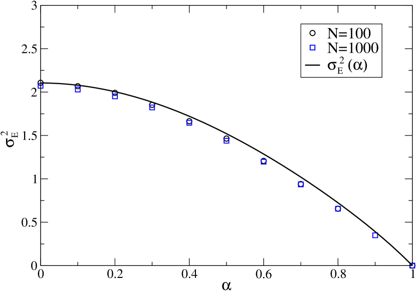
Figure 9: Plot of $\sigma^{2}_{E}$ versus the restitution coefficient $\alpha$ for $N=100$ ($\bigcirc$) and $N=1000$ ($\square$) particles, for the Gaussian thermostat. The solid line shows the theoretical predictions of brey04a , given by Eq. (43).

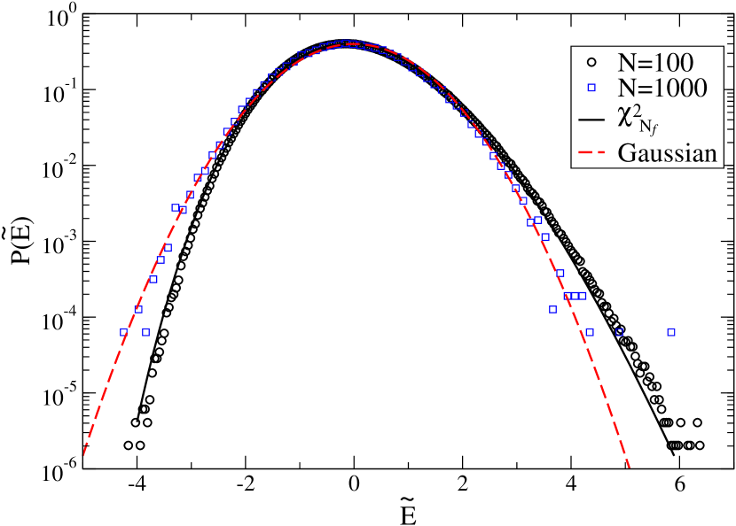
Figure 10: pdf of the rescaled energy $\widetilde{E}$ when the restitution coefficient is $\alpha=0.5$. The system is driven with the Gaussian thermostat with 100 ($\bigcirc$) and 1000 ($\square$) particles. The solid line shows a rescaled gamma distribution with zero-mean, a variance equal to 1, and with a number of degrees of freedom $N_{f}$ given by $2N/\sigma_{E}^{2}$. The dashed line is the Gaussian with zero-mean and unit variance.

4 Conclusion

In this paper, we have investigated the fluctuations of the total kinetic energy of granular gases maintained in a non-equilibrium stationary state through various kinds of energy injection mechanisms. For heating through a boundary, the system remains inhomogeneous, and the characteristic function of the energy pdf can be analytically computed as a functional of the temperature profile of the system, under the assumption that the particle velocities are uncorrelated. Despite this approximation, the use of the hydrodynamic profiles obtained in brey00c allows to recover results in agreement with the numerical simulations carried out in Ref. aumaitre04 . This result seems to hold even if the hydrodynamic approximation is not valid in the whole volume of the system, in particular near the vibrating wall. Moreover, we find that the effective temperature defined in aumaitre04 , which is measurable, is intensive only if the number of layers of particles is large enough, and can be related to a quantity which plays the role of the “temperature of the vibrating wall”, which is microscopically not well defined, and a priori not measurable. An effective number of degrees of freedom can be also defined, and its dependence on the true number of degrees of freedom has been obtained. Once again, the obtained behavior is in agreement with the numerical simulations described in aumaitre04 , and leads to the conclusion that the non-extensive behavior of the total energy in such a system is essentially due to the density and temperature inhomogeneities and can be understood through a hydrodynamic approach.

In homogeneously driven granular gases the total energy displays a $\chi^{2}$ pdf, with a number of degrees of freedom proportional to the number of particles. The total energy is hence extensive, and moreover, in the $N\to\infty$ limit the $\chi^{2}$ distribution tends to the Gaussian. We measured, by means of DSMC simulations, the rescaled variance $\sigma_{E}^{2}$ of the energy pdf, which depends only on the restitution coefficient. These non-trivial fluctuations are essentially due to the correlations induced by the inelasticity of the particles. We can distinguish between two different contributions to these correlations. First, the non-Gaussianity of the velocity pdf, which simply tells that the Euclidean components of the velocity of each particle are correlated one to each other. Second, a contribution from the two particles velocity pdf, which does not factorize exactly as a product of two one-particle distributions. The analytical computation of the rescaled variance $\sigma_{E}^{2}$ under the assumption of uncorrelated non-Gaussian individual velocity pdfs does not reproduce the DSMC results, showing the relevance of this second contribution. It must be pointed out, however, that these correlations do not invalidate the Boltzmann equation. As already noted in ernst81 ; brey04a , the two points correlation function $g_{2}({\bf v}_{1},{\bf v}_{2})$, which is defined by:

$$g_{2}({\bf v}_{1},{\bf v}_{2})=f^{(2)}({\bf v}_{1},{\bf v}_{2})-f({\bf v}_{1})f({\bf v}_{2})\,\,,$$ (45)

where $f^{(2)}$ is the two points distribution, is of higher order in the density expansion (roughly speaking ${\cal O}\left(g({\bf v}_{1},{\bf v}_{2})\right)\sim{\cal O}\left(f({\bf v}_{1})f({\bf v}_{2})\right)/N$). This is confirmed by the numerical observation, since the energy pdf tends to a Gaussian when the number of particles increases.

When the gas is heated with the Gaussian thermostat, the numerical results are in good agreement with the analytical result in brey04a . This means in particular that the DSMC algorithm is able to capture effects arising from the two-particle velocity pdf, which is remarkable. Moreover the energy pdf obtained with DSMC coincides with its counterpart found in MD simulations in the dilute limit, provided the system remains homogeneous (cf. Fig. 8). This feature is consistent with the fact that the DSMC algorithm exactly simulates the homogeneous pseudo-Liouville equation governing the $N$-particle dynamics of the gas.

For the gas thermostated by a random noise, numerical simulations show that the quantity $\sigma_{E}^{2}$ behaves in a fashion similar to what happens for the Gaussian thermostat. Nevertheless in the elastic limit ($\alpha\to 1$) it tends to a non trivial value ($\sim d/\sqrt{2}$), which is still not understood. An analytical calculation of $\sigma_{E}^{2}$ is in principle possible, exploiting the methods described in brey04a . Nevertheless, in order to carry on with such methods, one needs the expression of the eigenfunctions of the linearized Boltzmann operator. While for the Gaussian thermostat these eigenfunctions can be computed, in the way as for the elastic hard sphere gas, this task seems more demanding in the case of a stochastically driven granular gas.

- (1) Z.A. Rácz, Proc. SPIE Int. Soc. Opt. Eng. 5112, 248 (2003)
- (2) S.T. Bramwell, P.C.W. Holdsworth, J.F. Pinton, Nature 396, 552 (1998)
- (3) J. Brey, M. de Soria, P. Maynar, M. Ruiz-Montero, Phys. Rev. Lett. 94, 098001 (2005)
- (4) A. Barrat, E. Trizac, M.H. Ernst, J. Phys. Condens. Matter 17, S2429 (2005)
- (5) T. Pöschel, S. Luding, eds., Granular Gases (Springer, Berlin, 2001), Lecture Notes in Physics 564
- (6) T. Pöschel, N. Brilliantov, eds., Granular Gas Dynamics (Springer, Berlin, 2003), Lecture Notes in Physics 624
- (7) W. Losert, D.G.W. Cooper, J. Delour, A. Kudrolli, J.P. Gollub, Chaos 9(3), 682 (1999), cond-mat/9901203
- (8) F. Rouyer, N. Menon, Phys. Rev. Lett. 85(17), 3676 (2000)
- (9) A. Kudrolli, J. Henry, Phys. Rev. E 62(2), R1489 (2000), cond-mat/0001233
- (10) R.D. Wildman, D.J. Parkar, Phys. Rev. Lett. 88(19), 064301 (2002)
- (11) J.J. Brey, M.J. Ruiz-Montero, F. Moreno, Phys. Rev. E 62, 5339 (2000)
- (12) E. Bertin, Phys. Rev. Lett. 95, 170601 (2005)
- (13) M.H. Ernst, E.G.D. Cohen, J. Stat. Phys 25(1), 153 (1981)
- (14) J. Brey, M. de Soria, P. Maynar, M. Ruiz-Montero, Phys. Rev. E 70(011302) (2004)
- (15) E.L. Grossman, T. Zhou, E. Ben-Naim, Phys. Rev. E 55, 4200 (1997)
- (16) S. McNamara, J.L. Barrat, Phys. Rev. E 55, 7767 (1997)
- (17) S. McNamara, S. Luding, Phys. Rev. E 58, 813 (1998)
- (18) V. Kumaran, Phys. Rev. E 57(5), 5660 (1998)
- (19) A. Barrat, E. Trizac, Phys. Rev. E 66(5), 051303 (2002)
- (20) S. Aumaître, J. Farago, S. Fauve, S. McNamara, Eur. Phys. J. B 42, 255 (2004)
- (21) W. Feller, Probability Theory and its Applications (John Wiley & Sons, New York, 1971)
- (22) M. Abramowitz, I.A. Stegun, Handbook of mathematical functions with formulas, graphs and mathematical tables (Dover, New York, 1972)
- (23) S. Aumaître, S. Fauve, S. McNamara, P. Poggi, Eur. Phys. J. B 19, 449 (2000)
- (24) D.R.M. Williams, F.C. MacKintosh, Phys. Rev. E 54(1), R9 (1996)
- (25) T.P.C. van Noije, M.H. Ernst, Granular Matter 1(2), 57 (1998)
- (26) A. Puglisi, V. Loreto, U.M.B. Marconi, A. Vulpiani, Phys. Rev. E 59, 5582 (1999)
- (27) T.P.C. van Noije, M.H. Ernst, E. Trizac, I. Pagonabarraga, Phys. Rev. E 59, 4326 (1999)
- (28) J.M. Montanero, A. Santos, Granular Matter 2(2), 53 (2000), cond-mat/0002323
- (29) S.J. Moon, M.D. Shattuck, J.B. Swift, Phys. Rev. E 64, 031303 (2001), cond-mat/0105322
- (30) V. Garzo, J.M. Montanero, Physica A 313(3-4), 336 (2002)
- (31) F. Cecconi, F. Diotallevi, U.M.B. Marconi, A. Puglisi, J. Chem. Phys. 120, 35 (2004)
- (32) D.J. Evans, G.P. Morriss, Statistical Mechanics of Nonequilibrium Liquids (Academic Press, London, 1990)
- (33) F. Coppex, M. Droz, J. Piasecki, E. Trizac, Physica A 329, 114 (2003)
- (34) A. Goldshtein, M. Shapiro, J. Fluid Mech. 282, 75 (1995)
- (35) J.F. Lutsko, Phys. Rev. E 63, 061211 (2001)