Ice: a strongly correlated proton system

Abstract

We discuss the problem of proton motion in Hydrogen bond materials with special focus on ice. We show that phenomenological models proposed in the past for the study of ice can be recast in terms of microscopic models in close relationship to the ones used to study the physics of Mott-Hubbard insulators. We discuss the physics of the paramagnetic phase of ice at $1/4$ filling (neutral ice) and its mapping to a transverse field Ising model and also to a gauge theory in two and three dimensions. We show that H${}_{3}^{+}$O and HO^- ions can be either in a confined or deconfined phase. We obtain the phase diagram of the problem as a function of temperature $T$ and proton hopping energy $t$ and find that there are two phases: an ordered insulating phase which results from an order-by-disorder mechanism induced by quantum fluctuations, and a disordered incoherent metallic phase (or plasma). We also discuss the problem of decoherence in the proton motion introduced by the lattice vibrations (phonons) and its effect on the phase diagram. Finally, we suggest that the transition from ice Ih to ice XI observed experimentally in doped ice is the confining-deconfining transition of our phase diagram.

I Introduction

Hydrogen bonds (or H-bond) are ubiquitous in physics, chemistry, and biology. The nature of H-bonds was studied in great detail by Pauling who predicted the mixed chemistry of H-bonds pauling , namely, H-bond shares characteristics of ionic and covalent bonds. On the one hand, a water molecule has a large dipole moment due to the electronegative character of the O atom and therefore water molecules are attracted to each other. This is the classical aspect of the H-bonding. On the other hand, the sigma bonding between H and O is strongly covalent with clear quantum mechanical nature. In the process of formation of an ice crystal electrons from the sigma bond can be shared by two water molecules leading to a strong link between them. Compton scattering experiments have confirmed the quantum nature of H-bonds in ice crystals cova . It has been clear since the early experiments in H-bond systems that although the physics of electrons in ice is important petrenko the protons are actually responsible for the amazing electrical properties of ice hobbs . The current understanding of the motion of protons in H-bond materials is mainly based in a few phenomenological models. In this paper we discuss a qualitative microscopic model which captures the basic quantum mechanical correlations of the proton system.

We show that the physics of protons in ice is a clear example of a strongly correlated problem very similar to the ones discussed in strongly correlated electron systems Fradkinbook reminiscent of the physics of Mott insulators mott . More specifically, the motion of protons in ice is hindered by strong constraints that forbid single proton hopping and only allows for collective ring-exchange-like motion. This sort of systems are known to be closely related to the physics of gauge theories. As we will see below, in the phase of ice in which the protons are ordered, in analogy with the problem of confinement of quarks in hadronic matter, pairs of defects (anions and cations) cost an energy which is linear with the separation between them.

Although there is a vast literature on physics of ice hobbs , we focus only on the quantum motion of protons. The concepts introduced here can be easily extended to the study of many different problems in H-bond materials. Ice shows many different solid phases depending on temperature and pressure. These phases are essentially controlled by the geometry of the H-bonds that link different water molecules. Furthermore, a H atom is located asymmetrically relative to the two O atoms, forming a double well structure in the bond. Thus, a H atom can sit in any of the two sides a bond. Hence, we can think of ice as made out of protons, H⁺, moving in a crystal lattice made out of O^-2 ions. Therefore, solids made out of H-bonds are expected to have strong electrical properties. For example, ice exhibits a high static permittivity comparable with the one of liquid water, electrical mobility that is large when compared to most ionic conductors (in fact, the mobility is comparable to the electronic conduction in metals). These are striking properties since in the solid phase only protons can move in an ice lattice as the electrons form a band insulator petrenko .

A striking feature of ice is its extensive classical entropy at low temperatures hobbs . This large entropy implies a macroscopic number of classically degenerate states at low temperatures. This is a situation very similar to frustrated magnetic systems, which the best representative is precisely called spin ice model Harris ; gingras . Our study, however, focus entirely on the proton motion in ice and not on magnetism. As we show, the proton motion in ice can be mapped into a problem with pseudo-spins, in close analogy to some frustrated magnets.

The most successful explanation for the physical behavior of ice was given by the phenomenological work of Bernal and Fowler bf in 1933 that gave rise to the so-called Bernal-Fowler (BF) rules: (i) the orientation of H₂O molecules is such that only one H atom lies between each pair of O atoms; (ii) each O atom has two H atoms closer to it forming a water molecule. Rule (i) prevents situations in which a H-bond has two H atoms. Rule (ii) does not allow for configurations in which each O has more than two H close to it. As it was shown by Pauling pauling , using a classical counting argument, these rules can account for most of the entropy measured in the experiments, and predict an extensive entropy even at $T=0$. A more detailed calculation taking into account ring exchange of protons in ice crystal brings this number even closer to the measured value nagle . Pauling’s statistical model has been very successful in explaining the distribution of protons in ice and has been confirmed experimentally in nuclear magnetic resonance (NMR) and neutron scattering experiments NMR .

Although Pauling’s calculation explains the arrangement of protons in ice it fails to describe its electrical properties. The reason for this failure is due to the fact that any motion of the protons under the BF rules requires an extremely correlated behavior ihm . In order to explain the electrical behavior another phenomenological concept was introduced, namely, the concept of defects. Defects, by definition, are local violations of the BF rules. The defects associated with violation of rule (i) are called Bjerrum defects bjerrum and the ones associated with violations of rule (ii) are called ionization defects defect . With the concept of defects one is able to explain most of the electrical properties of ice hobbs .

Protons can move by the rigid rotation of the water molecule, by thermal activation over an energy barrier from one side of the H-bond to another, or by quantum tunneling under the energy barrier between the two sides of the bond. At low temperatures, the rigid motion of the molecule and thermal activation are exponentially suppressed and only quantum tunneling is allowed. Quantum tunneling is possible because the wavefunction of the proton is extended from one side to another in the bond. Although the phenomenological theories of ice can account for a great part of the experimental data there are still many experiments that remain unexplained such as anomalies in the specific heat in pure giauque and doped ice pick . Originally it was proposed by Onsager onsager that these anomalies could be explained by a ferroelectric transition. It turns out, however, that there is no evidence for any polar effect in ice. Quite to the contrary, the BF rules state that ice is a rather non-polar material. In this paper we show that by a quantum mechanical mechanism of order-by-disorder, an ordered phase of protons emerges at low temperatures. The melting of this ordered state can account for the specific heat anomalies.

The classical ice model is defined on a pyrochlore lattice and its planar representation is the checkerboard lattice. The planar model is equivalent to the six vertex model what has been solved exactly by Lieb Lieb . It is known from these studies that the phase diagram of the classical planar system has two phases, an ordered anti-ferroelectric phase and a line of critical points with extensive entropy at zero temperature. The anti-ferroelectric phase corresponds to a staggered arrangement of proton positions in the H-bonds. Its quantum version has been studied by Moessner, Sondhi MS and collaborators others ; olav .

In this paper, we consider the quantum version of the ice problem and show that quantum fluctuations stabilize the anti-ferroelectric phase in the absence of defects by a mechanism of order-by-disorder. To this end, we use a gauge theory description of the planar quantum ice problem which can be easily extended to higher dimensional systems. This gauge theory has also being used in similar models such as the quantum dimer models on the square lattice Fradkinbook .

This paper is organized as follows: In the next section we discuss the characteristic energy scales of the ice problem and propose the minimal model for proton motion in ice. Here we discuss in detail the analogy and connection to frustrated quantum magnets. Section III contains the mapping of the planar ice model to a gauge theory. In Section IV we determine the ground state of the problem in the neutral sector. Here we show how an ordered state of protons arises from the order-by-disorder mechanism and how the ionic defects are confined in the planar model. In Section V we discuss the gauge problem in three dimensions and obtain the phase diagram including thermal effects. We show that the three dimensional case has a confining-deconfining transition even at T=0. In Section VI we briefly discuss the effects of lattice vibrations on the proton motion. We argue that the second order phase transitions obtained in the case without phonons can become first order. Section VII contains our conclusions and the comparison between the theory and the experimental measurements in hexagonal (Ih) ice.

II The model

Consider a lattice with protons living in the bonds and where each vertex is to be interpreted as an O atom as shown in Fig.1. The lattices we are going o discuss in this papers are the planar square lattice, the cubic lattice and the pyrochlore lattice. The protons can occupy two positions in their respective link. Let us divide any of those lattices into sub-lattices 1 and 2, and for each link $i$ define the sites $i1$ and $i2$ neighboring a vertex of sub-lattice 1 and 2, respectively. We can define the proton occupation number $n_{i,a}$, $a=1,2$ for each proton site $ia$ of the system.

The main energy scales in this problem come from the Coulomb repulsion between the protons: the on-site Coulomb repulsion, $U_{H}$ (the so-called Hubbard term), the Coulomb repulsion between protons in the same H-bond, $U_{B}$, and the Coulomb repulsion between protons around the same O vertex, $U_{O}$ lekner . The physical situation of interest for ice corresponds to the case where $U_{H}\gg U_{B}\gg U_{O}$. Notice that this condition ensures that there is only one proton per lattice site, only one proton per bond, and for $1/4$ filled ice it implies that there are only two protons around the O vertex. Thus, the electrostatic repulsion between the protons leads to the ice rules.

Since we have considered interactions up to second nearest neighbors one might wonder whether we should not include interactions with even longer range. In fact, it is well-known that the water molecules interact through long-range dipole forces that in our picture would be represented by long-range interactions between H⁺ ions. The same problem arises in the context of spin-ice gingras ; gingraslongrange . Monte carlo simulations montecarlo for the frustrated lattices discussed here have shown that the long-range dipolar interactions ”average out” to zero at large distances. This result shows that the ice rules are still obeyed in the absence of long-range interactions and that the degeneracy of the classical state is not lifted. Moreover, improved Monte Carlo simulations with ”non-local” updates detected the appearance of long range order only at very low energies, much smaller than the energy scales discussed here nonlocal . Thus, from now on the effects of long-range interactions between second nearest neighbors will be disregarded.

The Bjerrum and ionic defects mentioned earlier only occur if the protons hop from site to site. There are essentially only two types of hopping in this lattice: hopping on the H-bond with energy $t_{B}$ and hopping across the O vertex, $t_{O}$. Because the hopping energy is an exponential function of the distance it is easy to show that $t_{B}\gg t_{O}$. The presence of $t_{B}$ allows for the hopping of the protons around the O vertices leading to the creation of ionic defects. The hopping $t_{O}$, on the other hand, allows for two protons in the same H-bond and therefore can lead to Bjerrum defects. The values of $t_{B}$ and $t_{O}$ are much smaller than in electronic systems because of the much larger proton mass. Thus, we expect that $U_{O}\gg t_{B}$ making the proton motion analogous to the motion of electrons in Mott insulators.

Figure 1: Planar ice model: the vertices are O sites and the dots are H sites. The symbols are explained in the text.

In what follows we assume that $U_{H}\gg U_{B}\to\infty$ and $t_{B}\gg t_{O}\to 0$ so that only ionic defects are possible in the problem. It is also clear that in this limit the classical ground state obeys the ice rules and that magnetic phenomena associated with the proton spin does not play any role. Within the assumption that the on-site Coulomb repulsion between protons is very large, we restrain to the case where $n_{ia}=0,1$, $\forall i$ and the proton spin degrees of freedom can be ignored. The Hamiltonian for the proton motion on neutral planar ice with just one proton per bond, that is,

$$n_{i1}+n_{i2}=1\,,$$ (1)

is written as,

$${\cal H} = U_{O}\sum_{\langle i,j\rangle}\left(n_{i1}n_{j1}+n_{i2}n_{j2}\right)$$ (2)

$$- t_{B}\sum_{i}\left(c^{{\dagger}}_{i1}c_{i2}+h.c.\right)\,.$$

We now make use of the constraint Eq.(1), and define pseudo-spin operators associated to link $i$ as (we use units such that $k_{B}=1=\hbar$):

$$S_{i}^{x} = \frac{1}{2}\left(c^{{\dagger}}_{i1}c_{i2}+h.c.\right)\,,$$

$$S_{i}^{y} = \frac{i}{2}\left(c^{{\dagger}}_{i1}c_{i2}-h.c.\right)\,,$$

$$S_{i}^{z} = \frac{1}{2}\left(c^{{\dagger}}_{i1}c_{i1}-c^{{\dagger}}_{i2}c_{i2}\right)\,,$$ (3)

which, due to condition Eq.(1), obey the spin algebra $[S_{i}^{x},S_{j}^{y}]=i\delta_{i,j}S_{i}^{z}$. In terms of these operators the Hamiltonian of Eq.(2) is written as

$${\cal H}=J\sum_{\langle i,j\rangle}S_{i}^{z}S_{j}^{z}-\Gamma\sum_{i}S_{i}^{x}\,,$$ (4)

where $J=2U_{O}$ and $\Gamma=2t_{B}$. In the limit of $\Gamma=0$ the ground state is highly degenerate because there are many configurations of the pseudospins that give the same energy. One possible configuration is shown in Fig.2.

Figure 2: A possible configuration of the pseudospins that satisfies the BF rules.

By a duality transformation, in which each link corresponds to a vertex of the square dual lattice, it is easy to show that Eq.(4) describes also the Ising model in a transverse field on a lattice where now the spins are defined on vertices. In the case of the planar ice system, this lattice correspond to the checkerboard lattice (see Fig.3), while for the pyrochlore and cubic lattices one obtains corner sharing tetrahedra and hexades, respectively. It is clear that the ground state of the Hamiltonian of Eq.(4) with $\Gamma=0$ is an eigenstate of the operator $S^{z}$. This state corresponds the proton localized everywhere in either side of the link. In order to minimize the energy the distribution of protons is such that the only contributing configurations have the total magnetization of each vertex is equal to zero. For the pyrochlore and planar lattices, this means that each O has two protons close to it and two away. For the cubic lattice one would have three protons close to the O and three away. The number of configurations that satisfy the ice rules grows exponentially with the size of the system. Taking the planar case as an example, there are $\left(4/3\right)^{3N/2}$ of them Lieb .

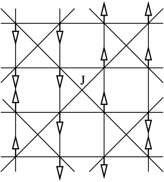
Figure 3: Effective spin lattice for the ice problem in the Mott regime. The pseudospins interact with an antiferromagnetic exchange $J$.

In the checkerboard language (see Fig.3) a sublattice of plaquettes contains next nearest neighbor interactions (“crossed plaquettes”). According to the BF rules the plaquettes have total $S^{z}$ magnetization equal to $0$ as shown in Fig.4(a). The configurations that contain defects violate the ice rules as shown in Figs.4(b) and (c). Classically, as it is well known, the system without defects corresponds to the six vertex model (see Fig.4(a)). The full classical problem is a 14 vertex model that, as far as we know, has not been solved exactly baxter .

Let us pick, for example, a particular configuration of the system that satisfies the ice rule and let us flip a single proton. This creates a pair of $+$ (H₃O⁺) and $-$ (OH^-) ionic charges at two neighboring O sites, corresponding to the configurations Fig.4(c) and Fig.4(b), respectively. Strictly at $\Gamma=0$, one can separate the $+$ and $-$ defects along a zig-zag-like trajectory at no extra energy cost. There is however an entropic price for separating such defects that introduces an effective interaction between them. These charge defects play the role similar to holons in quantum dimer models Fradkinbook . Two natural questions arise in this context. The first one concerns possible lifting of the degeneracy of the ground-states by quantum fluctuations when $t_{B}$ or $\Gamma$ are finite. The second question is whether in the presence of these quantum fluctuations the ionic defects can be separately freely (unconfined) as in the classical case.

Figure 4: (a) Configurations of the pseudospins that obey the BF rules; (b) ionic defect with charge $-$ (OH^-); (c) ionic defect with charge $+$ (H₃O⁺).

To answer the first question, let us consider the operator $P$ that projects into the subspace of states that satisfies the ice rules. Let $PHP^{-1}$ denote the Hamiltonian of Eq.(4) projected onto the ice rules sector, and let us treat the effects of finite $\Gamma$ in perturbation theory. The effective Hamiltonian, for the planar and cubic lattices, to the lowest non-vanishing order is (${\bf S}=\vec{\sigma}/2$):

$$H_{eff}=-t\sum_{\square}\left(\sigma_{ij}^{+}\sigma_{jk}^{-}\sigma_{kl}^{+}\sigma_{li}^{-}+h.c.\right)\,,$$ (5)

where $ij$ denote the links belonging to a crossed plaquette. To lowest order we find $t~{}\sim~{}\Gamma^{4}/J^{3}$. For the pyrochlore lattice, the lowest order effective Hamiltonian is:

$$H_{eff}=-t\sum_{ijklmn}\left(\sigma_{ij}^{+}\sigma_{jk}^{-}\sigma_{kl}^{+}\sigma_{lm}^{-}\sigma_{mn}^{+}\sigma_{ni}^{-}+h.c.\right)\,,$$ (6)

where now the interaction is around an hexagonal plaquette corresponding to the smallest loop in the pyrochlore lattice, and $t~{}\propto~{}\Gamma^{6}/J^{5}$. The planar lattice with the Hamiltonian of Eq.(5) has been studied at zero temperature $T=0$ MS . It can be mapped onto a height model in which quantum fluctuations select the ordered flat state corresponding to a Néel order in the checker-board model. It is worth mentioning that the effective Hamiltonian of Eq.(5) and Eq.(6) also describe tunneling within the low energy manifold of the $XXZ$ spin $1/2$ model on the checkerboard. To see that, we start by writing the $XXZ$ Hamiltonian:

$$H=\sum_{<ij>}\left(J_{z}S^{z}_{i}S^{z}_{j}+{J_{xy}\over 2}(S^{+}_{i}S^{-}_{j}+S^{-}_{i}S^{+}_{j})\right)\,,$$ (7)

where $<ij>$ stand for all the couple of links belonging to the checkerboard lattice. We assume $J_{xy}\ll J_{z}$. At zeroth order in $J_{xy}$ the ground state manifold is identical to the one mentioned before, with total $S^{z}$ magnetization per crossed plaquette equal to zero. Considering then the $XY$ term in the first non-vanishing order in perturbation theory leads to Eq.(5) with $t~{}\propto~{}J_{xy}^{2}/J_{z}$ and Eq.(6) with $t~{}\propto~{}J_{xy}^{3}/J_{z}^{2}$, respectively.

III Mapping of the planar quantum model to a lattice gauge theory

In this section we map the ice problem onto a gauge theory kogut ; fradkin . Consider the O lattice which is shown schematically in Fig.1. The H-bonds form links between the O atoms and to each link we can assign a value given by the pseudo spin defined in the previous section. Associated with these links we can assign states corresponding to the two configurations of the protons in each link which we will denote as $|+1/2\rangle$ and $|-1/2\rangle$. The ice rules imply

$$\sum_{i\in\square}\sigma^{z}_{i}=0\,,$$ (8)

where $\sigma_{z}|\pm 1/2\rangle=\pm|\pm 1/2\rangle$. This Ising gauge theory is equivalent to the one considered in Ref. [MSF, ], and as in that case, it has a local $U(1)$ symmetry generated by the unitary operator

$${\cal U}_{v}=\prod_{\alpha_{v}}e^{i\alpha_{v}\sum_{i\in v}\sigma^{z}_{i}}\,,$$ (9)

with each $\alpha_{v}$ associated to the vertex $v$ being arbitrary. This approach has been applied with success in the case of the quantum dimer model MSF .

There is an alternative and complementary approach which works in an enhanced Hilbert space and that was applied originally to the quantum dimer model as well Fradkinbook ; steve . Let us consider a square lattice is spanned by vectors ${\bf r}=(n{\bf e}_{1}+m{\bf e}_{2})a$ where $n$ and $m$ are integers, ${\bf e}_{1}={\bf x}$, ${\bf e}_{2}={\bf y}$ and $a$ is the lattice spacing. On each link (i.e., H-bond) we define a variable $\tilde{\ell}_{\mu}({\bf r})$ with $\mu=1,2$ which can be $-1/2$ or $1/2$, which transfer like a vector: $\tilde{\ell}_{-\mu}({\bf r}+{\bf e}_{\mu})=-\tilde{\ell}_{\mu}({\bf r})$. It will be convenient to define a new variable $\ell_{\mu}=\tilde{\ell}_{\mu}+1/2$ which can take values of $0$ or $1$. Let us denote by $\Delta_{\mu}$ the discrete derivative,

$$\Delta_{\mu}\ell_{\nu}({\bf r})=\ell_{\nu}({\bf r}+{\bf e}_{\mu})-\ell_{\nu}({\bf r})\,.$$ (10)

It is easy to see that the ice rules are equivalent to impose the condition that

$$\sum_{\mu=1,2}\Delta_{\mu}\ell_{\mu}({\bf r})=0\,.$$ (11)

Only configurations of the form Fig.4(a) are allowed for $\tilde{\ell}_{\mu}$. Therefore, Eq.((11) reflects the BF rules.

Eq.(11) has the form of Gauss law in electrodynamics without external charges, $\nabla\cdot{\bf E}=0$. We will then assign to violations of the ice rules, such as those in Fig.4(c) the condition of $\sum_{\mu=1,2}\Delta_{\mu}\ell_{\mu}({\bf r})=+1$ for the formation of a H${}^{+}_{3}$O and $\sum_{\mu=1,2}\Delta_{\mu}\ell_{\mu}({\bf r})=-1$ for the formation of HO^-. Thus, if we allow violations of the ice rules by formation of ionization “defects” we must have $\sum_{\mu=1,2}\Delta_{\mu}\ell_{\mu}({\bf r})=Q$ where $Q$ plays the role of the “effective” charge of the defect. In the quantum theory we define a Hilbert space of states $|\ell_{\mu}({\bf r})\rangle$ which are the eigenstates of the operator $E_{\mu}({\bf r})$:

$$E_{\mu}({\bf r})|\ell_{\mu}({\bf r})\rangle=\ell_{\mu}({\bf r})|\ell_{\mu}({\bf r})\rangle\,.$$ (12)

In the quantum theory Gauss law is a constraint in the space of state:

$$\sum_{\mu=1,2}\Delta_{\mu}E_{\mu}({\bf r})|{\rm Phys.}\rangle=0\,,$$ (13)

which defines the physical states of the system. Let $\theta_{\nu}$ be the operator canonically conjugated to $E_{\mu}$,

$$\left[\theta_{\nu}({\bf r^{\prime}}),E_{\mu}({\bf r})\right]=i\delta_{{\bf r},{\bf r^{\prime}}}\delta_{\mu,\nu}\,.$$ (14)

Thus, we see that $E_{\mu}$ plays the role of the electric field while $\theta_{\nu}$ plays the role of the vector potential in electrodynamics.

Let us now define a ring exchange operator such that it maps configuration of electric fields satisfying the ice rule conditions. In this context this amounts to require that these operators, when acting on a plaquette, change the configuration in a manner consistent with Eq.(13). For each plaquette $p$ we define the operator $e^{i\Phi(p)}$ where

$$\Phi(p)=\sum_{{\bf r},\mu\in p}\theta_{\mu}({\bf r})\,.$$ (15)

This operator is gauge invariant in the sense that it commutes with the generator of gauge transformations, $\Delta_{\mu}E_{\mu}({\bf r})$. When acting on the links one gets,

$$e^{\pm i\Phi(p)}|\ell_{\mu}({\bf r})\rangle=|\ell_{\mu}({\bf r})\pm 1\rangle\,.$$ (16)

We are now going to relax the constraint that $\ell_{\mu}({\bf r})$ can be $0$ or $1$ by enlarging the Hilbert space to all integer values of $\ell_{\mu}({\bf r})$. However, we will penalize energetically the values of $\ell_{\mu}({\bf r})$ that are not $0$ or $1$ by adding an extra term to the Hamiltonian of the form:

$$H_{0}=\frac{1}{2g}\sum_{{\bf r},\mu}\left[\left(E_{\mu}({\bf r})-\frac{1}{2}\right)^{2}-\frac{1}{4}\right]\,.$$ (17)

It is obvious that when $g\to 0$ $\ell_{\mu}({\bf r})$ can only be $0$ or $1$. Together with the constraint of Eq.(13), Eq.(17) defines the classical problem and the BF rules. Note that, for example, the Néel state corresponds to a configuration of electric fields in which the links (horizontal and vertical) form a staggered configuration of flux 0 and 1. These fluxes form stair like lines (right-up-right-up…) winding around the system. We also note that if the $1/2$ term in the kinetic energy Eq.(17) where not present, this problem would be equivalent to compact electrodynamics with matter fields studied in Refs. [kogut, ; fradkin, ]. The quantum kinetic energy of this problem is given by:

$$H_{I}=-t\sum_{p}\cos\Phi(p)\,,$$ (18)

which is analogous to the magnetic energy in compact electrodynamics.

In order to introduce ionic “defects” one has to introduce the charge $Q$ into the problem. Associated with $Q$ one defines the quantum operator $n({\bf r})$, which counts the number of defects at each vertex, and its conjugate $\phi({\bf r})$ such that

$$\left[\phi({\bf r^{\prime}}),n({\bf r})\right]=i\delta_{{\bf r^{\prime}},{\bf r}}\,.$$ (19)

where $n({\bf r})=0,\pm 1,\pm 2,...$ The Hamiltonian for the “matter” field $\phi$ contains a term for the energy required to create any one of these charges. For instance, one could write,

$$H_{Q}=E_{0}\sum_{\bf r}n^{2}({\bf r})\,,$$ (20)

where $E_{0}$ is the energy required to create a OH^--H${}^{+}_{3}$O pair. Observe that Eq.(20) tends to suppress defects. The motion of the defects is given by a kinetic energy term which is

$$H_{C}=\lambda\sum_{{\bf r},\mu}\cos\left(\Delta_{\mu}\phi({\bf r})-\theta_{\mu}({\bf r})\right)\,,$$ (21)

where $\lambda\sim\Gamma$ is the coupling constant. This kinetic energy is gauge invariant since it commutes with the generator of local gauge transformations

$$U=e^{i\sum_{{\bf r}}\alpha({\bf r})\hat{G}({\bf r})}\,,$$ (22)

where

$$\hat{G}({\bf r})=\sum_{\mu=1,2}\Delta_{\mu}E_{\mu}({\bf r})-n({\bf r})\,.$$ (23)

The gauge theory of the ice problem is described by the Hamiltonian $H=H_{0}+H_{I}+H_{Q}+H_{C}$ defined by Eqs. (17), (18), (20), and (21). In the next section we are going to study the ground state of such a theory in the neutral sector fendley .

IV Ground-state selection in the neutral sector and confinement

It is interesting to consider the analysis of the $U(1)$ lattice gauge theory of quantum dimer models given in Refs. [Fradkinbook, ; steve, ] in the context of our calculation. In the neutral sector, since the electric field has zero divergence, it can be written as:

$$E_{\mu}{\bf r})=\epsilon_{\mu\nu}\left[\Delta_{\nu}S({\bf r})+B_{\nu}({\bf r})\right]\,,$$ (24)

where $S$ is an integer valued function defined on the dual lattice with periodic boundary conditions and $B_{\nu}$ is defined on the links of the dual lattice. Since the Gauss law tells us that

$$\epsilon_{\mu\nu}\Delta_{\mu}B_{\nu}=0\,,$$

only non-trivial topological configurations of $B_{\nu}$ have to be considered. Let us choose, in particular, $B^{N}_{\nu}$ constructed in the following way: let us define $B^{N}_{\mu}$ for $\mu=2$ to take the alternating values $0$ and $1$ on vertical links from row to row. For horizontal links with $\mu=1$, $B^{N}_{\mu}$ will alternate from $0$ and $-1$ in such a way that each positive oriented arrow in the vertical direction meets a negative oriented arrow in the horizontal direction (see Fig.5). By choosing such a $B^{N}_{\nu}$ and choosing $S=0$ on the dual sites one gets for $E_{\mu}$ one of the two Néel configuration (the other configuration being obtained by assigning a $0,1$ staggered value to $S$).

Figure 5: Background field $B^{N}_{\mu}$.

We can now write the path integral representation in discrete imaginary time in the form of the a 3-D discrete Gaussian model:

$${\cal S} = {1\over 2t\epsilon}\sum_{{\bf r},j}\left[\Delta_{0}S({\bf r},j)\right]^{2}$$ (25)

$$+ {\epsilon\over 2g}\sum_{{\bf r},j,\mu=1,2}\left[\Delta_{\mu}\left(S({\bf r},j)-S^{0}\right)\right]^{2}\,,$$

where $j$ is the discrete time coordinate ($\epsilon$ and $\Delta_{0}$ are the “lattice spacing” and the discrete derivative in the imaginary time direction, respectively), and $S^{0}$ is a staggered configuration alternating between $0$ (in say, sub-lattice “A”) and $1/2$ (in sub-lattice “B”). While a non-zero $t$ allows for fluctuations of the field $S$, only some kind of fluctuations can be made without paying the energy of the huge “surface tension” $1/g$. More precisely, if at some point of sub-lattice “A” the value of $S$ is 0, then the neighboring values of $S$ (belonging to sub-lattice “B”) can fluctuate between the values $-1$ and $0$ with no cost in surface tension.

Imagine now that we consider the most general situation for the electric field Eq.(24) in which the vector field $B_{\mu}$ has a non-trivial winding. The action for the discrete Gaussian model becomes :

$${\cal S} = {1\over 2t\epsilon}\sum_{{\bf r},j}\left[\Delta_{0}S({\bf r},j)\right]^{2}$$ (26)

$$+ {\epsilon\over 2g}\sum_{{\bf r},j,\mu=1,2}\left[\Delta_{\mu}\left(S({\bf r},j)-S^{0}\right)-B_{\mu}\right]^{2}\,.$$

Let us also assume that we choose the configuration for $B_{\mu}$ with the minimal number of links where it is non-zero. One can show that, for any configuration with non-zero $B_{\mu}$, either there is no configuration of the $S$ degrees of freedom that minimizes the surface tension term at each point, or at each point connected to a link where $B_{\mu}$ is non-zero, there is a unique value for the field $S({\bf r},j)$ (modulo a global constant) that satisfies both periodic boundary conditions and a minimal surface tension. In the limit $g\rightarrow 0$ the values of the field $S$ associated to those points are not allowed to fluctuate. Then, the computation of the partition function of a discrete Gaussian model in a topological sector having non-zero $B_{\mu}$ is penalized by the surface tension term or gives rise to the freezing of some of the plaquette degrees of freedom $S({\bf r},j)$ which gives a smaller contribution than the sector $B_{\mu}=0$ (since the configuration space of the former is a subset of the later). Keeping in mind these arguments, from now on, we are going to consider only the sector $B_{\mu}=0$.

To deal with the discrete variable $S$ we make use of the Poisson summation formula:

$$\sum_{n=-\infty}^{\infty}f(n)=\sum_{m=-\infty}^{\infty}\int~{}d\phi~{}e^{i2\pi m\phi}f(\phi)\,,$$ (27)

and write the partition function:

$$Z\sim\sum_{\{m\}}\int~{}D\phi~{}\exp({\cal S}(m,\phi))\,,$$ (28)

where,

$${\cal S} = \sum_{{\bf r},j}\left\{i2\pi m({\bf r},j)\phi({\bf r},j)-{1\over 2t\epsilon}\left[\Delta_{0}\phi({\bf r},j)\right]^{2}\right.$$ (29)

$$- \left.{\epsilon\over 2g}\sum_{\mu=1,2}\left[\Delta_{\mu}\left(\phi({\bf r},j)-S^{0}\right)\right]^{2}\right\}\,.$$

We redefine: $\tilde{\phi}=\phi-S^{0}$, and write $\tilde{\phi}$ as $\tilde{\phi}_{A}$ and $\tilde{\phi}_{B}$ for sub-lattices A and B, respectively. Following Ref. [RS, ], we work on the dilute gas approximation and keep only “monopoles” of charge $\pm 1$. In this case one finds an effective action of the form:

$${\cal S} = \sum_{{\bf r},j}\left\{{\epsilon\over 2g}\left(\tilde{\phi}_{A}-\tilde{\phi}_{B}\right)^{2}+{1\over 2t\epsilon}\left(\left[\Delta_{0}\tilde{\phi}_{A}\right]^{2}+\left[\Delta_{0}\tilde{\phi}_{B}\right]^{2}\right)\right.$$ (30)

$$- \left.z~{}\cos(2\pi\tilde{\phi}_{A})+z~{}\cos(2\pi\tilde{\phi}_{B})\right\}\,,$$

where $z$ is the monopole fugacity. In order to take the continuum limit, we write

$$\tilde{\phi}_{A}=\chi_{1}+\chi_{2}~{}~{},~{}~{}\tilde{\phi}_{B}=\chi_{1}-\chi_{2}\,,$$ (31)

Note that a non-zero expectation value for $\chi_{2}$ corresponds to the two Néel orders depending on the sign of $<\chi_{2}>$ while $<\chi_{2}>=0$ corresponds to a disordered state. Expanding in derivatives of the fields we get a continuum action of the form:

$${\cal S} = \int d^{2}\vec{r}d\tau\left\{\frac{1}{2}\left[K_{x}(\nabla\chi_{1})^{2}+K_{\tau}(\partial_{\tau}\chi_{1})^{2}+\alpha~{}\chi_{2}^{2}\right]\right.$$ (32)

$$+ \left.\lambda~{}\sin(2\pi\chi_{1})\sin(2\pi\chi_{2})\right\}\,.$$

Where $\nabla$ is the spatial two-dimensional gradient, $K_{x}$, $K_{\tau}$, $\alpha$, and $\lambda$ are the parameters of the effective coarse grained model that in principle, but with a large amount of effort, can be calculated from the microscopic theory. Here the continuum limit has being taken with the prescriptions:

$$\Delta_{0}\chi({\bf r},j) \rightarrow \epsilon\partial_{\tau}\chi({\bf r},\tau)+{\cal O}(\epsilon^{2})\,,$$

$$\chi({\bf r}+a{\bf e}_{\mu},j) \rightarrow \chi({\bf r},\tau)+a{\bf e}_{\mu}\cdot\nabla\chi({\bf r},\tau)+{\cal O}(a^{2})\,,$$

$$\displaystyle\sum_{j}\epsilon \to \int d\tau\,\,{\rm and}\displaystyle\sum_{{\bf r}}a^{2}\to\int d^{2}{\bf r}\,,$$

where $a$ is the lattice spacing. We have not written the time and space variations of the field $\chi_{2}$ because this field is massive and therefore the low energy physics is dominated by the $\chi^{2}_{2}$ term. Because of that we can integrate out the $\chi_{2}$ term in perturbation theory in $\lambda$ in order to generate an effective field theory for the field $\chi_{1}$. In this case we obtain a relativistic-like field theory of the form:

$${\cal S}_{\rm{eff}} = \int d^{2}\vec{r}d\tau\left\{\frac{K}{2}\left[(\nabla\chi_{1})^{2}+(\partial_{\tau}\chi_{1})^{2}\right]\right.$$ (33)

$$- \left.\gamma\cos(4\pi\chi_{1})\right\}\,,$$

where, $K$ is the stiffness, and $\gamma=\pi\lambda^{2}/(2\alpha)$ (we have set the velocity of propagation of the field equals to one, for simplicity). Eq. (33) describes a Sine-Gordon problem in $2+1$ dimensions. Notice that in $2+1$ dimensions the stiffness has dimensions of energy and, since the only energy scale in this problem is the hopping $t$ (since $g\to 0$), one concludes that $K\propto t$.  note Since we have assumed that $\gamma\ll 1$ we can study this problem using a renormalization group argument Polyakov ; kosterlitz , that is, we study the relevance of the cosine operator perturbatively by integrating high energy modes in a shell between $\Lambda$ and $\Lambda+d\Lambda$ where $\Lambda$ is the ultraviolet cut-off of the theory. In doing that the coupling $\gamma$ renormalizes as Polyakov ; kosterlitz :

$$\frac{d\gamma}{d\ell}=\gamma^{2}\,,$$ (34)

where $d\ell=d\Lambda/\Lambda$. Hence, $\gamma$ is a marginally relevant coupling indicating that the field $\chi_{1}$ is “frozen” at the minima of the potential in (33), that is, at $\langle\chi_{1}\rangle=\pm 1/4$ and a gap opens in the spectrum of $\chi_{1}$ (thus, both $\chi_{1}$ and $\chi_{2}$ are massive). The above result could be also derived directly from (32) by minimizing the potential energy in order to find:

$$\langle\chi_{1}\rangle=\mp 1/4~{};~{}\langle\chi_{2}\rangle=\pm{\pi\lambda\over\alpha}\cos(2\pi\langle\chi_{2}\rangle).$$ (35)

Thus, the energetic cost of instanton configurations in this systems forces it to freeze on one of the configurations that minimizes the potential. As mentioned before, the resulting ground-states present the Néel order. Thus, we have shown by a mechanism of order-by-disorder that the classical degeneracy is lifted by quantum fluctuations and select a state with Néel order. This conclusion is consistent with numerical simulations others ; olav .

To understand what is the effect of a finite temperature, it is better to come back to the discrete action (32). We fist notice that the coarse grained system has effective $Z_{2}\otimes U(1)$ symmetry, corresponding to changing $\chi_{2}\to-\chi_{2}$ and $\chi_{1}\to\chi_{1}+n/2$ (where $n$ is an integer). The ground state occurs with the simultaneous breaking of the two symmetries leading to a flat configuration of the fields. As the temperature is increased we expect the restoration of the $Z_{2}$ symmetry and a rough phase with algebraic correlations for the $\chi_{1}$ field. The effective two-dimensional action at finite temperatures has the form:

$${\cal S} = \beta\int d^{2}\vec{r}d\tau\left\{\frac{1}{2}\left[K(\nabla\chi_{1})^{2}+\alpha(\chi_{2})^{2}\right]\right.$$ (36)

$$+ \left.\lambda\sin(2\pi\chi_{1})\sin(2\pi\chi_{2})-\gamma\cos(4\pi\chi_{1})\right\}\,.$$

where $\beta=1/T$ is the inverse temperature. Clearly, the phase transition from a disordered high temperature phase to the ordered low temperature phase occurs with the breaking of the $Z_{2}\otimes U(1)$ symmetry. As usual, the critical temperature, $T_{c}$, is proportional to the stiffness $K$ and therefore, $T_{c}\propto K\propto t$, consistent with the statement that $t$ is the only physical energy scale in this problem.

Equation (33) also allows us to see explicitly how defects that are created over such ground state are confined by following Polyakov’s argument Polyakov . While this is a result that one could easily anticipated from the nature of the ground state itself, its description in terms of a gauge theory will be useful in higher dimensional models discussed in the next section. As we argued above, and as also considered in similar systems on Ref. [RS, ], we look for an effective action of the field $\chi_{1}$ which couples to the matter field (the defects). Integrating over the massive field $\chi_{2}$ and expanding $\tilde{\chi}=\chi_{1}-<\chi_{1}>$ in Eq.(33) we obtain the effective action:

$${\cal S}=\int d\vec{r}d\tau\left\{\frac{K}{2}\left[(\nabla\tilde{\chi})^{2}+(\partial_{\tau}\tilde{\chi})^{2}\right]+m^{2}~{}\tilde{\chi}^{2}\right\}\,,$$ (37)

where $m^{2}\approx 2\pi^{2}\gamma$. These fluctuations are then massive and decay over a length scale $\sim 1/m$ reflecting the fact that two-component Coulomb gas has Debye screening. This is also the confinement scale which defines the string tension $\sigma$ of the defects, that is, the confining potential has the form: $V(R)=\sigma R$ where $\sigma\sim m$. This argument follows from Polyakov’s analysis Polyakov of the standard compact QED in $2+1$ dimensions which gives the same effective action as in Eq.(37). At finite temperature, as long as the system remains in the flat phase, the ionic defects will be confined. Increasing further the temperature will make the system enter the rough phase, at which the effective theory can be described by a massless theory for the field $\chi_{1}$ with $U(1)$ symmetry Lieb . Creation operators of ionic defects correspond to vertex operators of the dual fields (or dislocations in the surface roughening language) which now have algebraic decaying correlation functions.

V Three-dimensional models

In $3+1$ dimensions the situation is more interesting since there is a confining-deconfining transition in the normal compact QED at $T=0$. It is then in the cubic and pyrochlore lattice where we do have a chance to see deconfined ionic excitations even at $T=0$. This argument has been used recently by Hermele et al. in the context of the spin ice on the pyroclore lattice HFB . The simplest three-dimensional lattice where we can apply this description is the cubic lattice. On this lattice, we can in fact write the Hamiltonian with precisely the same form as in $2+1$ dimensions. The main difference with the standard QED is again the term in Eq.(17) which penalizes configurations with $E_{\mu}\neq 0,1$. In Ref. [HFB, ], numerical evidence is provided that due to this term in Eq.(17) the defects are deconfined, which is to say that in the current model corresponds to a quantum disordered phase of ice (proton liquid). However, this analysis is based on a “naive” continuum limit of a lattice model and therefore is only applicable deep in the deconfined phase. It is known from early studies of compact QED in $3+1$ dimensions that this theory has a deconfinement-confinement quantum phase transition at a critical value of the coupling constant $t$, the resonance amplitude lautrup ; kogut82 . Qualitatively this phase transition is driven by the proliferation of “monopole loops”. Notice that the theory described here, being perturbative in $t$, cannot describe the details of the quantum critical point that occurs at finite values of $t$. Nevertheless, these general arguments do predict the existence of a deconfinement-confinement quantum transition at finite $t=t_{c}$ and $T=0$ fradkin . The actual location of this quantum critical point may be controlled by additional operators not included here, such as the short range part of the dipole interaction, which affect the “electric” terms but leave the “magnetic” (flip) terms untouched. It is likely that the model we are considering here, which has a single coupling constant $t$, with the electric terms playing the role of a constraint, may be in the deconfined (or “Maxwell”) phase.

The proton phases of ice are characterized by the energy required to separate two defects with opposite sign. In the confined phase (the ordered phase of ice) the energy grows linearly with the separation between the ions. Therefore, in this phase it is not possible to separate the H₃O⁺ and HO^- ions at arbitrary distance with the application of an external electric field. This state is a dielectric with a finite polarizability and it is an insulator. However, in the deconfined phase the effective interaction between the ions obeys $V(R)\propto 1/R$ and therefore decreases with the distance between the ions. Thus, in this case an applied electric field can separate the two H${}^{+}_{3}$O and HO^- ions at arbitrary distance leading to a conducting state. Hence, the phase transition is a metal-insulator transition mott and therefore the conductivity of ice should behave quite different in the two different sides of the transition. We should note that in the metallic phase the conduction is due to the collective motion of protons. This is a correlated metal.

In Fig.6 we depict the phase diagram of ice as a function of temperature and the proton hopping energy $t$. In Fig.6(a) we show the phase diagram for planar ice ($2+1$ dimensions) for which we have shown that there is no deconfining transition as a function of $t$ at $T=0$. As we argued in the last section, there will be, however, a phase transition at finite temperature $T_{c}$ ($T_{c}\propto t$ for $t\to 0$) between the disordered metallic phase and the ordered insulating phase. In the case at hand, the arguments presented above indicate the presence of a line of second order phase transition conjecture . As we are going to see in the next Section, the coupling to phonons can change the transition to first order. In the case of the pyroclore or cubic lattice ($3+1$ dimensions) we have argued that there is a confining deconfining transition as a function of $t$, as shown in Fig.6(b). In this case, there is a quantum critical point (QCP) at some value of $t$ (say, $t_{c}$).

\psfrag{T}{$T$}\psfrag{Tc}{$T_{c}$}\psfrag{t}{$t$}\psfrag{tc}{$t_{c}$}\psfrag{QCP}{QCP}\psfrag{Deconfined}{Deconfined Disordered}\psfrag{Plasma}{Proton Plasma}\psfrag{Confined}{Confined Ordered}\psfrag{Insulator}{Proton Insulator}\includegraphics[width=151.76964pt,keepaspectratio]{phase_diagram-2d.eps}

\psfrag{T}{$T$}\psfrag{Tc}{$T_{c}$}\psfrag{t}{$t$}\psfrag{tc}{$t_{c}$}\psfrag{QCP}{QCP}\psfrag{Deconfined}{Deconfined Disordered}\psfrag{Plasma}{Proton Plasma}\psfrag{Confined}{Confined Ordered}\psfrag{Insulator}{Proton Insulator}\includegraphics[width=151.76964pt,keepaspectratio]{phase_diagram-3d-new.eps}

Figure 6: Phase diagram for protons in neutral ice. (a) Planar ice; (b) Three dimensional ice.

VI Coupling to lattice vibrations

So far we have not discussed the problem of lattice vibrations in ice. At finite temperatures one expects that the thermal motion of the O atoms to affect the properties of the H atoms. Vibrations must be important since the mass of the H atoms are just 16 times smaller than the O atoms and therefore the Born-Oppenheimer approximation is not guaranteed. In order to incorporate the recoil of the O atoms due to the H motion we assume that the phonon coordinates are coupled to the local proton density. In this case, one has to add an extra term to the Hamiltonian of the form:

$$H_{P}= - \kappa\sum_{i,\alpha,\sigma}n_{i,\alpha,\sigma}q_{i,\alpha,a}$$ (38)

$$+ \sum_{i,\alpha,a}\left(\frac{P_{i,\alpha,a}^{2}}{2M}+\frac{M\omega_{i,a}q_{i,\alpha,a}^{2}}{2}\,,\right)$$

where $q_{i,\alpha,a}$ are the local phonon coordinates, $P_{i,\alpha,a}$ their canonical momentum, $\omega_{i,a}$ are the phonon frequencies, and $M$ the ion mass. Eq.(38) can be reduced to the two level system in the same way Eq.(2) is reduced to Eq.(4). Using Eq.(3) and defining the relative and center of mass coordinates:

$$x_{i,a} = q_{i,1,a}-q_{i,2,a}\,,$$

$$X_{i,a} = \frac{q_{i,1,a}+q_{i,2,a}}{2}\,,$$ (39)

the Hamiltonian Eq.(38) reduces to

$$H_{P} = -\kappa\sum_{i,a}S_{i}^{z}x_{i,a}+\sum_{i,a}\left(\frac{p_{i,a}^{2}}{M}+\frac{M\omega_{i,a}x_{i,a}^{2}}{8}\right.$$ (40)

$$+ \left.\frac{\Pi_{i,a}^{2}}{4M}+\frac{M\omega_{i,a}X_{i,a}^{2}}{4}\right)\,,$$

where $p_{i}$ is conjugated to $x_{i}$ and $\Pi_{i}$ is conjugated to $X_{i}$. Notice that the center of mass coordinate decouples from the proton motion in this case.

It is interesting to rewrite the full Hamiltonian of the problem in terms of the pseudo-spin operators and standard creation $b^{{\dagger}}_{i}$ and annihilation $b_{i}$ operator for the phonons ($[b_{i},b^{{\dagger}}_{j}]=\delta_{ij}$). Using Eq.(4) and proton-phonon coupling term Eq.(40) we find:

$$H = J\sum_{\langle i,j\rangle}S^{z}_{i}S^{z}_{j}-\Gamma\sum_{i}S^{x}_{i}+\sum_{i,a}\lambda_{i,a}S^{z}_{i}(b_{i,a}+b_{i,a}^{{\dagger}})$$ (41)

$$+ \sum_{i,a}\omega_{i,a}b^{{\dagger}}_{i,a}b_{i,a}$$

where $\lambda_{i,a}=\kappa/\sqrt{M\omega_{i,a}}$. Eq.(41) describes an Ising model in a transverse field coupled to a dissipative environment à la Caldeira-Leggett caldeira . This model has been studied recently in the context of quantum phase transitions in metallic magnetic systems griffiths ; leticia and has very interesting properties.

Let us consider the classical case of $\Gamma\ll J$ when the ice rules are obeyed. In this case the problem can be solved in the basis of $S^{z}$: $S^{z}_{j}|\sigma_{j}\rangle=\sigma_{j}|\sigma_{j}\rangle$. It is easy to see that the problem can be diagonalized by shifting operators:

$$B_{j,a} = b_{j,a}+\frac{\lambda_{j,a}\sigma_{j}}{\omega_{j,a}}\,,$$

$$B^{{\dagger}}_{j,a} = b^{{\dagger}}_{j,a}+\frac{\lambda_{j,a}\sigma_{j}}{\omega_{j,a}}\,,$$ (42)

and the energy of the problem is given by:

$$E[\{\sigma,n\}] = J\sum_{\langle i,j\rangle}\sigma_{i}\sigma_{j}$$ (43)

$$+ \sum_{i,a}\left[\omega_{i,a}\left(n_{i,a}+\frac{1}{2}\right)-\frac{\lambda_{i,a}^{2}}{\omega_{i,a}}\right]$$

where the first term is just the energy of the classical state and $n_{i,a}$ is the phonon number. So, the phonon frequencies remain the same but the atoms positions are shifted by $\delta x_{i,a}\propto\kappa\sigma_{i}/(M\omega_{i,a}^{2})$. Since there is no proton order when $\Gamma=0$ the average lattice shift is zero. However, for a small value of $\Gamma$ we see from Fig. 6 that $\sigma_{i}$ acquires an average expectation value leading to an overall shift in the atom positions. At finite temperature this shift will lead to a discontinuity in the specific heat as it is well known in the case of cooperative transitions of this sort cooptrans . Thus, the phase diagram second order phase transition of Fig.6 can be modified substantially. In $2+1$ dimensions the finite temperature phase transition can change completely to first order while in $3+1$ dimensions a tricritical point must appear at some temperature $T^{*}$ so that for $T<T^{*}$ the phase transition is second order and for $T>T^{*}$ the transition becomes first order.

VII Conclusions and Experimental Realizations

In this paper we have considered the phase diagram of protons in ice. We have given a detailed picture of two-dimensional ice and provide a qualitative picture of the three-dimensional problem such as the pyrochlore lattice. We have studied the order-by-disorder effect and ground-state selection by quantum fluctuations, which in this case is the tunneling of protons between the two sites in a Hydrogen bond.

In the absence of quantum tunneling, the number of low energy states grows exponentially with the size of the system and the entropy of the system is macroscopic. In this classical background, excited states corresponding to ionic defects can be created and separated without further cost in energy. As we showed, the presence of quantum fluctuations change considerably this scenario. The degeneracy of the system is lifted by the order-by-disorder mechanism leading to a well defined ground state. The technique used to understand the role of quantum fluctuations is based on a mapping of the lattice problem onto a gauge theory.

Within the gauge theory one can describe the behavior of ionic defects as confined or deconfined depending whether the ground state of the system is ordered or disordered, respectively. In a deconfined state the ionic defects behave like as in a correlated metal, while in the confined phase the system behaves as in an insulator. For the two-dimensional model, quantum fluctuations select a a two-fold degenerate antiferroelectric ground-state over which ionic excitations are confined. The situation is different in the three-dimensional case where topological excitations can lead to a deconfined disordered state even at $T=0$. In such case, the interplay of quantum fluctuations and the tuning of the microscopic tunneling parameter is expected to give rise to a confinement-deconfinement transition for ionic defects, with their corresponding dramatic effects in the dielectric properties of the material.

Furthermore, we have argued that at finite temperatures there will be a phase transition between ordered (confined) and disordered (deconfined) ice. The nature of this phase transition depends on the fugacity associated with the topological defects (monopoles) and can be either first or second order. In the pyroclore lattice the most likely scenario is that there is a tricritical point separating a first order from a second order phase transition (see Fig.6(b)) that should be observable. While similar problems have already being addressed in terms of spin models MS ; HFB , the ice scenario brings a new perspective to this kind of phenomenology due the more accessible experimental possibilities than in frustrated spins systems fulde .

It is clear from Fig.6(b) that the way to tune the phase transition is by changing the value of the proton hopping energy $t$. The value of $t$ depends on the overlap of the proton wavefunction between the two sites in the Hydrogen bond. Since the mass of the proton is large its wavefunction is more localized than in the electronic case and we expect that $t$ is exponentially sensitive on the changes in the distance between O atoms. One clear way to experimentally change $t$ is then by applying hydrostatic pressure $P$ to an ice crystal at fixed temperature $T$, starting from the disordered phase, and measuring the ice conductivity or dielectric response as a function of pressure. One expects that the proton ordering discussed here occurs at lower pressures than the well-known structural phase transitions of ice hobbs .

Another way to change the O-O distance is by using “chemical pressure” kawada . One can dope water with salts like KOH that while in solution become K⁺ and HO^-. When in the solid phase the K⁺ ion becomes trapped into the “cages” of O atoms while the HO^- ions are assimilated into the ice lattice. Thus, in this case, doping also introduces charges into the lattice structure and the ground state is no longer neutral. Furthermore, since the K⁺ ions spread randomly over the ice lattice, this kind of doping also introduces disorder in the system. The attractive interaction between the positive K⁺ ions and the negative O^-2 atoms of the ice structure lead to a local decrease of the volume of ice “cages”, to an average decrease in the H-bond distance, and to an average increase in $t$. So, in first approximation the introduction of KOH is somewhat equivalent to the horizontal axis in Fig.6. However, because there is introduction of charges and disorder in the system, the horizontal axis in Fig.6 is only roughly the concentration of KOH.

Doping experiments with KOH have been performed more than $20$ years ago kawada in order to understand the famous $72$ K anomaly observed in the temperature dependence of the specific heat of undoped ice dopspec . The specific heat of pure ice at low temperatures increases with temperature as $T^{3}$ which is the characteristic of phonons in the material. However, it has been known for a long time that hexagonal ice (ice-Ih) has a bump in the specific heat at $T\approx 72$ K that was a theoretical mystery onsager . By doping pure ice with KOH it was shown by Kawada in the 1970’s that the specific heat bump is actually a very slow phase transition into an ordered proton state that was called ice XI kawada ; structure . Permittivity experiments in doped ice have confirmed this scenario oguro . Specific heat measurements in KOH doped ice showed a strong and highly hysteretic first order phase transition with a substantial loss of entropy in the low temperature phase dopspec . Neutron scattering experiments on single crystals of ice have confirmed the ordering transition jackson ; D2O . While the critical temperature is weakly dependent on the amount of KOH, the loss of entropy is dependent on the KOH concentration. Furthermore, in accordance with our discussion in the previous section, the first order phase transition is associated with lattice distortions as seen in recent neutron scattering experiments phonons .

Hence, our theory provides a possible theoretical explanation for the phase transition between ice-Ih and ice-XI. We believe that the first order phase transition observed in the experiments is the one described in Fig.6(b) and it would be very interesting to find out whether the quantum critical point can be studied by further doping of KOH or by application of pressure. Our theory indicates that at $T\to 0$ and $t<t_{c}$ the protons in ice-Ih would make an unique state of matter, namely, a quantum proton liquid, with deconfined ion excitations.

- (1) L. Pauling, The Nature of the Chemical Bond (Cornell Press, Ithaca, 1960).
- (2) E. D. Isaacs, A. Shukla, P. M. Platzman, D. R. Hamann, B. Barbiellini and C. A. Tulk, Phys. Rev. Lett. 82, 600 (1999).
- (3) V. F. Petrenko and I. A. Ryzhkin, Phys. Rev. Lett. 71, 2626 (1993).
- (4) P. V. Hobbs, Ice Physics (Claredon Press, Oxford, 1974).
- (5) E. Fradkin, Field Theories of Condensed Matter Systems (Addison-Wesley, Redwood City, 1991).
- (6) N. F. Mott, Metal-Insulator Transitions (Taylor & Francis, London, 1974).
- (7) A. P. Ramirez, Annu. Rev. Mater. Sci. 24, 453 (1994); P. Schiffer and A. P. Ramirez, Comments Condens. Matter Phys. 18, 21 (1996); M. J. Harris and M. P. Zinkin, Mod. Phys. Lett. B 10, 417 (1996).
- (8) For a review on spin-ice, see S. T. Bramwell, and M. J. P. Gingras, Science 294, 1495 (2001), and references therein.
- (9) J. D. Bernal and R. H. Fowler, J. Chem. Phys. 1, 515 (1933).
- (10) J. F. Nagle, J. Math. Phys. 7, 1484 (1966).
- (11) K. Kume, J. Phys. Soc. Japan 15, 1493 (1960); K. Kume and R. Hoshino, J. Phys. Soc. Japan 16, 290 (1961); S. W. Rabideau and A. B. Denison, J. Chem. Phys. 49, 4660 (1968).
- (12) J. Ihm, J. Phys. A: Math. Gen. 29, L1 (1996).
- (13) N. Bjerrum, Science 115, 385 (1952).
- (14) In an electrically neutral ice crystal the formation of a cation like HO naturally leads to the formation of an anion HO-.
- (15) W. F. Giauque and J. W. Stout, J. Am. Chem. Soc. 58, 1144 (1936).
- (16) M. A. Pick, in Physics of ice, 344 (1969).
- (17) L. Onsager, in Ferroelectricity 16 (1967).
- (18) E. H. Lieb, Phys. Rev. Lett. 18, 1046, (1967).
- (19) R. Moessner and S. L. Sondhi, Phys. Rev. B 63, 224401, (2001).
- (20) R. Moessner, O. Tchernyshyov, and S. L. Sondhi, Jour. Stat. Phys. 116, 755 (2004).
- (21) Olav F. Syljuåsen, and Sudip Chakravarty, arXiv:cond-mat/0509624.
- (22) J. Lekner, Physica B 252, 149 (1998).
- (23) R. G. Melko, M. Enjalran, B. C. den Hertog, and M. J. P. Gingras, J. Phys.: Condens. Matter 16, R1277 (2004).
- (24) B. C. den Hertog and M. J. P. Gingras, Phys. Rev. Lett. 84, 3430 (2000).
- (25) R. G. Melko, B. C. den Hertog, and M. J. P. Gingras, Phys. Rev. Lett. 87, 067203 (2001).
- (26) R. J. Baxter, Exactly Solved Models in Statistical Mechanics (Academic Press, London, 1982).
- (27) J. B. Kogut, Rev. Mod. Phys. 51, 659, (1979).
- (28) E. Fradkin and S. H. Shenker, Phys. Rev.D 19, 3682, (1979).
- (29) R. Moessner, S. L. Sondhi and E. Fradkin, Phys. Rev.B 65, 024504, (2001).
- (30) E. Fradkin, and S. Kivelson, Mod. Phys. Lett. B 4, 225 (1990).
- (31) Similar results for gauge theories of dimer models with different quantum dynamics can be found in E. Ardonne, P. Fendley, E. H. Fradkin, Annals Phys. 310, 493 (2004).
- (32) N. Read and S. Sachdev, Phys. Rev.B 42, 4568, (1990).
- (33) The actual value of the stiffness cannot be directly calculated from the naive coarse grained theory in the continuum limit because its value is renormalized by fluctuations.
- (34) A. M. Polyakov, Nuc. Phys. B120, 429, (1977).
- (35) J. M. Kosterlitz, Jour. Phys. C 10, 3753 (1977).
- (36) M. Hermele, M. P. A. Fisher, and L. Balents, preprint cond-mat/0305401.
- (37) B. Lautrup, and M. Nauenberg, Phys. Rev. Lett. 45, 1755 (1980).
- (38) J. B. Kogut, Rev. Mod. Phys. 55, 755 (1983).
- (39) In Ref. [olav, ] it is conjectured that this transition is of first order, instead of second order.
- (40) A. O. Caldeira, and A. J. Leggett, Physica 121 A, 587 (1983).
- (41) A. H. Castro Neto, and B. A. Jones, Phys. Rev. B 62, 14975 (2000).
- (42) L. F. Cugliandolo, D. R. Grempel, G. Lozano, and H. Lozza, preprint cond-mat/0312064.
- (43) G. A. Gehring, and K. A. Gehring, Rep. Prog. Phys. 38, 1 (1975).
- (44) After the completion of this work we became aware of another work of charge motion in frustrated lattices: E. Runge and P. Fulde, unpublished.
- (45) S. Kawada, J. Phys. Soc. Jpn. 32, 1442 (1972).
- (46) Y. Tajima, T. Matsuo and H. Suga, Nature 299, 810 (1982); J. Phys. Chem. Solids 45, 1135 (1984); J. Phys. Chem. Solids 47, 165 (1986); M. Ueda, T. Matsuo and H. Suga, J. Phys. Chem. Solids 43, 1165 (1982).
- (47) The lattice structure remains pyroclore during the transition.
- (48) M. Oguro, R. W. Whitworth, J. Phys. Chem. Solids 52, 401 (1991).
- (49) S. M. Jackson, V. M. Nield, R. W. Whitworth, M. Oguro, and C. C. Wilson, Jou. Phys. Chem. B 101 6142 (1997).
- (50) The same order is observed in KOH doped D2O, see, H. Fukazawa, S. Ikeda, and S. Mae, Chem. Phys. Lett. 282, 215 (1998).
- (51) H. Fukazawa, S. Ikeda, M. Oguro, S. M. Bennington, and S. Mae, J. Chem. Phys. 118, 1577 (2003).