Local and chain dynamics in miscible polymer blends: A Monte Carlo simulation study

Abstract

Local chain structure and local environment play an important role in the dynamics of polymer chains in miscible blends. In general, the friction coefficients that describe the segmental dynamics of the two components in a blend differ from each other and from those of the pure melts. In this work, we investigate polymer blend dynamics with Monte Carlo simulations of a generalized bond-fluctuation model, where differences in the interaction energies between non-bonded nearest neighbors distinguish the two components of a blend. Simulations employing only local moves and respecting a non-bond crossing condition were carried out for blends with a range of compositions, densities, and chain lengths. The blends investigated here have long-chain dynamics in the crossover region between Rouse and entangled behavior. In order to investigate the scaling of the self-diffusion coefficients, characteristic chain lengths $N_{\mathrm{c}}$ are calculated from the packing length of the chains. These are combined with a local mobility $\mu$ determined from the acceptance rate and the effective bond length to yield characteristic self-diffusion coefficients $D_{\mathrm{c}}=\mu/N_{\mathrm{c}}$. We find that the data for both melts and blends collapse onto a common line in a graph of reduced diffusion coefficients $D/D_{\mathrm{c}}$ as a function of reduced chain length $N/N_{\mathrm{c}}$. The composition dependence of dynamic properties is investigated in detail for melts and blends with chains of length twenty at three different densities. For these blends, we calculate friction coefficients from the local mobilities and consider their composition and pressure dependence. The friction coefficients determined in this way show many of the characteristics observed in experiments on miscible blends.

I Introduction

Processes on different length scales affect dynamic properties of polymer melts and blends Doi and Edwards (1986); Grosberg and Khokhlov (1994); de Gennes (1979); Ferry (1980). The dynamics of miscible blends have been the subject of a large number of recent investigations with experimental (see, for example, Refs. Roland and Ngai, 1991, 1992; Chung et al., 1994a; He et al., 2003; Chung et al., 1994b; Alégria et al., 1994; Kim et al., 1995; Pathak, 2001; Min et al., 2001; Haley et al., 2003; Lutz et al., 2003; Haley and Lodge, 2004; Lutz et al., 2004; Alegría et al., 2002; Doxastakis et al., 2000; Genix et al., 2005), simulation (cf. Refs. Genix et al., 2005; Kopf et al., 1997; Kamath et al., 2003; Doxastakis et al., 2000; Budzien et al., 2002; Faller, 2004; Neelakantan et al., 2005), and theoretical methods (cf. Refs. Zetsche and Fischer, 1994; Katana et al., 1995; Kumar et al., 1996; Kamath et al., 1999; Lodge and McLeish, 2000; He et al., 2003; Leroy et al., 2003; Kant et al., 2003; Chung et al., 1994a; Roland and Ngai, 1991, 1992; Ngai and Roland, 2004; Luettmer-Strathmann, 2005). Monomeric friction coefficients, which are inversely proportional to the mobility of short chain segments, are a convenient way to describe the effect of local dynamic properties on global dynamic properties such as the viscosity Ferry (1980).

Since blending changes the local environment of the chain segments of a polymer it has a strong effect on the local dynamics of the chains. From experimental Roland and Ngai (1991, 1992); Chung et al. (1994a, b); Alégria et al. (1994); Kim et al. (1995); Doxastakis et al. (2000); Pathak (2001); Min et al. (2001); Haley et al. (2003); Lutz et al. (2003); Haley and Lodge (2004); Lutz et al. (2004); Alegría et al. (2002); He et al. (2003) and simulation work Kopf et al. (1997); Kamath et al. (2003); Doxastakis et al. (2000); Budzien et al. (2002); Faller (2004); Neelakantan et al. (2005); Genix et al. (2005) it is found that the local dynamics of the two blend components differ from each other and the pure melts. The addition of slow (high friction coefficient) component to a blend is found to increase the friction coefficients of both components and, conversely, the addition of fast component is found to speed up both components. The effects of blending are most pronounced near the glass transition, however, they are observed even at high temperatures Doxastakis et al. (2000); Min et al. (2001); Haley et al. (2003); Lutz et al. (2003) and in blends where one of the components is dilute Lutz et al. (2003, 2004); Haley and Lodge (2004).

Several recently developed models for miscible polymer blends relate differences in the component dynamics to local variations in the glass transition temperature induced by local variations in blend composition Zetsche and Fischer (1994); Katana et al. (1995); Kumar et al. (1996); Kamath et al. (1999); Lodge and McLeish (2000); He et al. (2003); Leroy et al. (2003); Kant et al. (2003), while others consider “intrinsic” effects, due to differences in the chain structure of the two components, in addition to local density and composition variations Chung et al. (1994a); Roland and Ngai (1991, 1992); Ngai and Roland (2004); Luettmer-Strathmann (2005). Unfortunately, it is still difficult, in general, to predict the local friction coefficients in a blend from those of the melts.

Self diffusion coefficients give information about the chain dynamics of polymer melts and blends. The Rouse model prediction for the self-diffusion coefficient of a polymer chain may be written as Doi and Edwards (1986); Grosberg and Khokhlov (1994).

$$D_{\mathrm{R}}=\frac{k_{\mathrm{B}}T}{\zeta N}=\frac{\mu}{N},$$ (1)

where $T$ is the temperature, $k_{\mathrm{B}}$ is Boltzmann’s constant, $N$ is the chain length, $\zeta$ is the so-called monomeric friction coefficient, and $\mu=k_{\mathrm{B}}T/\zeta$ is the corresponding mobility. The long-time dynamics of long polymer chains are dominated by entanglement effects, which are not part of the Rouse model. The reptation model Doi and Edwards (1986); Grosberg and Khokhlov (1994); de Gennes (1979) describes the entanglements of a chain with other chains in terms of a tube, which restricts the motion of the chain perpendicular to the tube. If the average number of monomers between entanglements is denoted by $N_{\mathrm{e}}$, then the reptation prediction for the self-diffusion coefficient takes the form

$$D_{\mathrm{G}}=\frac{k_{\mathrm{B}}TN_{\mathrm{e}}}{3N^{2}\zeta}=\frac{1}{3}\frac{N_{\mathrm{e}}}{N}D_{\mathrm{R}}.$$ (2)

The entanglement length of a polymer melt may be determined directly from experimental data on the plateau modulus Doi and Edwards (1986); Graessley and Edwards (1981). For viscoelastic properties, it differs by a constant prefactor from the characteristic chain length $N_{\mathrm{c}}$, that separates short chain (unentangled) behavior from long chain (entangled) behavior Graessley and Edwards (1981). Experimental, theoretical and simulation work on polymer melts suggests that the tube diameter of the reptation theories is proportional to the so-called packing length Lin (1987); Kavassalis and Noolandi (1987); Fetters et al. (1999); Everaers et al. (2004); Sukumaran et al. (2005); Milner (2005), which may be defined as Fetters et al. (1999); Everaers et al. (2004)

$$p=\frac{N}{\rho R_{e}^{2}},$$ (3)

where $\rho$ is the monomer density and $R_{e}^{2}$ is the average squared end-to-end vector of the chains. Hence, the entanglement length is expected to be proportional to the chain length corresponding to $p$, which yields Milner (2005)

$$N_{\mathrm{c}}\sim p^{3}\rho.$$ (4)

The transition between the unentangled and entangled regimes is not sharp and simulation data are often found to be in the crossover region between unentangled and reptation behavior Binder and Paul (1997); Müller et al. (2000); Tanaka et al. (2000); Kreer et al. (2001); Paul and Smith (2004); León et al. (2005). In the following, it is convenient to rescale the chain length $N$ by the characteristic chain length $N_{\mathrm{c}}\propto N_{\mathrm{e}}$ and the self-diffusion coefficient $D$ by a characteristic diffusion coefficient $D_{\mathrm{c}}$ defined as Müller et al. (2000),

$$D_{\mathrm{c}}=\frac{\mu}{N_{\mathrm{c}}}.$$ (5)

In this way, the predictions for the self-diffusion coefficient may be summarized as

$$\frac{D}{D_{\mathrm{c}}} = \left\{\begin{array}[]{lcl}\left({N}/{N_{\mathrm{c}}}\right)^{-1}&\textrm{ for }&N\ll N_{\mathrm{c}}\\ \left({N}/{N_{\mathrm{c}}}\right)^{-2}&\textrm{ for }&N\gg N_{\mathrm{c}}\end{array}\right.$$ (8)

so that, at the chain length $N_{\mathrm{c}}$, the extrapolations from both power laws yield the same value, $D/D_{\mathrm{c}}=1$. For long but not completely entangled chains, Hess Hess (1986, 1988) has proposed a crossover equation for the self-diffusion coefficient, which may be written in our notation as

$$\frac{D}{D_{\mathrm{c}}}=\frac{\displaystyle\left({N}/{N_{\mathrm{c}}}\right)^{-1}}{\displaystyle 1+{N}/{N_{\mathrm{c}}}}.$$ (9)

This expression has been found to give a good representation of data for self-diffusion coefficients of the bond-fluctuation model Paul et al. (1991). However, the resulting values for the characteristic chain length $N_{\mathrm{c}}$ are considerably smaller than those obtained by superimposing simulation data with experimental data that extends deeply into the entangled regime Tanaka et al. (2000).

Simulation work on polymer blends has been carried out with atomistic Doxastakis et al. (2000); Budzien et al. (2002); Faller (2004); Neelakantan et al. (2005); Genix et al. (2005) and coarse grained models Kopf et al. (1997); Kamath et al. (2003). Molecular dynamics simulations of atomistic models give access to the chain structure and dynamics of realistic polymers and allow a detailed investigation of the environments of the chain segments Neelakantan et al. (2005). Simulations of coarse grained models, on the other hand, can be used to isolate particular effects such as isotope effects Kopf et al. (1997) and differences in chain stiffness Kamath et al. (2003).

In this work, we investigate chain and local dynamics of miscible polymer blends with the aid of Monte Carlo simulations of a lattice model. We are interested in energetic effects and represent the two components of a blend by chains that differ only in interaction energies. The model is a modification of Shaffer’s bond-fluctuation model for athermal melts Shaffer (1994, 1995); Pan and Shaffer (1996) and is introduced in Section II. Section II also provides some details about the Monte Carlo simulations. In Section III we discuss the evaluation of the Monte Carlo simulations and describe the construction of scaling variables for the self-diffusion coefficients. Results of our simulations are presented in Section IV and discussed in Section V.

II Blend model for Monte Carlo simulation

Shaffer’s bond fluctuation model Shaffer (1994, 1995); Pan and Shaffer (1996) is a lattice model for polymer chains, where the monomers occupy sites of a simple cubic lattice. In the following, we will take the size of the unit cell, i.e. the lattice constant $a$, as the unit for length. The monomers are connected by bonds of three possible lengths, namely 1, $\sqrt{2}$, and $\sqrt{3}$, corresponding to the sides, face diagonals, and body diagonals of the unit cell of the lattice. Monte Carlo simulations of the model employ only local moves, where an attempt is made to displace a randomly chosen monomer by one lattice site along any of the three coordinate directions. One attempted elementary move per monomer in the system is called one Monte Carlo step (MCs) and will be our unit of time. Shaffer considered two versions of this model. In the first version, bonds are allowed to cross each other with the result that the chains do not entangle; in the second, bond crossings are prohibited and entanglement effects become apparent. We adopt the second approach and prohibit bond crossings in this work.

Figure 1: Illustration of the generalization of Shaffer’s bond fluctuation model to polymer blends. The circles connected by heavy lines represent polymer chains in a blend, gray for component A and black for component B. Allowed bond lengths are 1, $\sqrt{2}$ and $\sqrt{3}$ corresponding to the sides, face diagonals, and body diagonals of the unit cell of the simple cubic lattice. The arrows show examples of nearest neighbor interactions between like ($\epsilon_{AA}$ and $\epsilon_{BB}$) and unlike ($\epsilon_{AB}$) monomers.

Shaffer’s model describes athermal melts; the monomers interact only through hard core repulsion, which is enforced by prohibiting double occupation of lattice sites. Shaffer (1994) In this work, we are interested in blends of polymers that have identical bond structures but differ in their monomer-monomer interactions. To this end, we add attractive interactions between non-bonded monomers occupying nearest-neighbor sites to the model, see Fig. 1. For a binary blend of chains of type A and B, the energy parameters $\epsilon_{AA}$, $\epsilon_{BB}$, and $\epsilon_{AB}$, describe interactions between monomers of type A, type B, and mixed interactions, respectively. The total internal energy of the system is given by

$$E=N_{AA}\epsilon_{AA}+N_{BB}\epsilon_{BB}+N_{AB}\epsilon_{AB},$$ (10)

where $N_{ij}$, $i,j\in\{A,B\}$, denotes the number of nearest neighbor contacts between monomers of type $i$ and $j$. In this work, we choose $\epsilon_{AA}=-1\epsilon$, $\epsilon_{BB}=-2\epsilon$, and $\epsilon_{AB}=-2\epsilon$, where $\epsilon$ is the unit of energy. The large difference in the interaction energies $\epsilon_{AA}$ and $\epsilon_{BB}$ makes differences between A and B chains readily observable in simulations. The value of $\epsilon_{AB}$ corresponds to very attractive interactions between unlike monomers and insures the miscibility of the blends. From the temperature $T$, the unit of energy, $\epsilon$, and Boltzmann’s constant, $k_{\mathrm{B}}$, a dimensionless temperature $T^{*}$ and its inverse $\beta$ are defined as $T^{*}=k_{\mathrm{B}}T/\epsilon$ and $\beta=1/T^{*}$. In this work, we present blend simulation results for the fixed temperature $T^{*}=10$ corresponding to $\beta=0.1$.

For a cubic lattice with $L$ lattice sites on the side, the monomer density $\rho$ is defined as

$$\rho=\frac{N_{pA}N_{A}+N_{pB}N_{B}}{L^{3}},$$ (11)

where $N_{pA}$ and $N_{pB}$ are the number of chains, while $N_{A}$ and $N_{B}$ are the chain lengths for chains of type $A$ and $B$, respectively. The mass fraction $c_{A}$ of component $A$ in a blend is given by

$$c_{A}=\frac{N_{pA}N_{A}}{N_{pA}N_{A}+N_{pB}N_{B}}.$$ (12)

In this work, we consider only monodisperse melts and blends, i.e. $N_{A}=N_{B}\equiv N$, so that the mass fraction is equal to the mole fraction.

Shaffer established that a monomer density of $\rho=0.5a^{-3}$ corresponds to a dense melt for the athermal system Shaffer (1994). We performed Monte Carlo simulations for the three monomer densities $\rho=0.5a^{-3}$, $0.6a^{-3}$, and $0.7a^{-3}$ at $\beta=0.1$. For melts and 50/50 blends, we considered nine chain lengths between $N=5$ and $N=80$. For intermediate concentrations, we focused on chains of length $N=20$. Simulations were performed on a lattice of size $L=20$ with periodic boundary conditions applied along the three coordinate directions. In order to test for finite size effects, we performed simulations for chains of length $N=80$ in a 50/50 blend on a lattice of size $L=40$ and found no significant differences in the results.

Initial configurations were created by randomly placing dimers on the lattice and repeatedly reassembling shorter chains into longer chains, where the no bond-crossing condition was enforced from the start. These initial configurations were equilibrated at the inverse temperature $\beta=0.1$ before a trajectory of the simulation consisting of 10,000 configurations separated by a fixed number of Monte Carlo steps, $t_{r}$, was recorded. The number of Monte Carlo steps during production varied between $10^{6}$ for the shortest chains and $10^{8}$ for the longest chains. Typical simulation times for chains of length $N=20$ are $10^{7}$ Monte Carlo steps. In order to improve the statistics for blends, where the mass fraction of one of the components is very small (5%), simulation times were extended to at least $5\times 10^{7}$. In all simulations, the equilibration time was at least 10% of the production time and was sufficiently long for the chains to travel a distance corresponding to multiple times the radius of gyration. During the simulations, the acceptance rates $A_{\text{rate}}$ for elementary moves are monitored separately for each of the components.

III Evaluation of simulation results

The Monte Carlo simulations are evaluated to yield static and dynamic quantities. The average radius of gyration, $R_{g,A}$, of chains of type A, for example, is calculated from

$$R_{g,A}^{2}=\frac{1}{N_{pA}}\sum_{k=1}^{N_{pA}}\frac{1}{N^{2}}\sum_{i<j}\langle(\mathbf{r}_{i,k}-\mathbf{r}_{j,k})^{2}\rangle,$$ (13)

where $\mathbf{r}_{i,k}$ is the position of monomer $i$ on chain $k$ of component A, and where the angular brackets indicate the average over configurations in the trajectory. The calculation for the radius of gyration of chains of type B proceeds in the same way. In order to simplify notation, we drop the subscripts indicating the type of chain whenever the calculation is identical for both components in the blend and there is no danger of confusion. Error estimates for static quantities are obtained from block averaging Newman and Barkema (1999), where we divide the trajectories into ten equal blocks.

In melts and miscible blends, polymer chains of sufficient length are expected to obey Gaussian statistics. For such chains, the average squared end-to-end distance $R_{e}^{2}$ is proportional to the number of bonds, $R_{e}^{2}=b^{2}(N-1)$, where $b$ is the so-called effective bond length Doi and Edwards (1986). Since the squared averages of the radius of gyration and end-to-end distance for dense systems are related through $R_{e}^{2}=6R_{g}^{2}$, we calculate the effective bond length from

$$b^{2}=6R_{g}^{2}/(N-1).$$ (14)

For Gaussian chains, the packing length defined in Eq. (3) may be expressed as $p=\left(\rho b^{2}\right)^{-1}$, where $\rho$ is the monomer density defined in Eq. (11). This allows us to calculate an estimate for the characteristic chain length $N_{\mathrm{c}}$ from Eq. (4)

$$N_{\mathrm{c}}=C_{c}\left(b^{3}\rho\right)^{-2},$$ (15)

where the constant of proportionality, $C_{c}$, is determined from a comparison with the crossover equation (9) of Hess Hess (1986, 1988).

In this work, we present results for two mean-squared displacement functions. The mean squared displacement of the center of mass is obtained from

$$g_{d}(t)=\frac{1}{N_{p}}\sum_{k=1}^{N_{p}}\langle(\mathbf{r}_{\mathrm{cm},k}(t)-\mathbf{r}_{\mathrm{cm},k}(0))^{2}\rangle,$$ (16)

where $\mathbf{r}_{\mathrm{cm},k}$ is the position of the center of mass of chain $k$ and where the angular brackets indicate the average over configurations that are $t$ Monte Carlo steps apart. Similarly, the mean squared displacement of the central monomer is obtained from

$$g_{1}(t)=\frac{1}{N_{p}}\sum_{k=1}^{N_{p}}\langle(\mathbf{r}_{N/2,k}(t)-\mathbf{r}_{N/2,k}(0))^{2}\rangle$$ (17)

where $\mathbf{r}_{N/2,k}$ represents the position of the central monomer of the chain (the results are averaged over both innermost monomers for chains with an even number of monomers).

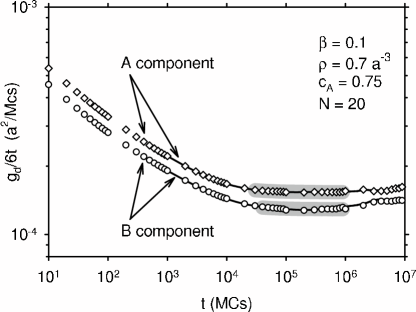
Figure 2: The function $g_{d}/6t$, where $g_{d}$ is the mean squared displacement and $t$ is the time, as a function of time for an A-rich blend with mass fraction $c_{A}=0.75$, monomer density $\rho=0.7a^{-3}$, inverse temperature $\beta=0.1$, and chain length $N=20$. The symbols indicate results for the two components, A (diamonds) and B (circles), obtained with the block algorithm during the simulation. The black lines represent results from the evaluation of the trajectory, which is limited to times larger than the recording interval $t_{r}=10^{3}$ MCs and agrees well with the results from the block algorithm. The gray areas show the ranges of $g_{d}/6t$ data that were used to determine the self-diffusion coefficients of the two components as explained in the text.

The self-diffusion coefficients of the components are determined from the long-time limit of mean-squared displacement $g_{d}$ of the center of mass

$$D=\lim_{t\rightarrow\infty}\frac{g_{d}(t)}{6t}.$$ (18)

In Fig. 2 we present simulation results for $g_{d}/6t$ for both components of an A-rich blend ($c_{A}=0.75$) of chains of length $N=20$ at a monomer density of $\rho=0.7$ and an inverse temperature of $\beta=0.1$. The results in Fig. 2 were calculated by two different methods. During the simulations, a block algorithm adapted from Frenkel and Smit Frenkel and Smit (1996) was used to determine mean squared displacements. The algorithm yields values of the displacement functions at intervals that increase with increasing time and, thus, gives access to a large time range. These values are indicated by open symbols in Fig. 2. We also calculated displacement functions from the trajectories at the time intervals $t_{r}$ for times up to half the total run time. These results are represented by solid lines in Fig. 2. The graphs show that the values for $g_{d}/6t$ obtained by the two methods agree well with each other. The block algorithm is very efficient and was used to determine most of the self-diffusion coefficients presented in this work. The results for $g_{d}/6t$ decrease with time at short times before they level off to a constant value and, finally, become irregular at very long times. The decrease of $g_{d}/6t$ at short times indicates the subdiffusive behavior expected for shorter chains Kreer et al. (2001); Paul (2002). For very long times, the results for the displacement functions are irregular since they represent averages over few configurations so that individual events, like the release of a chain from entanglements, can alter the shape of the functions McCormick et al. (2005). The $g_{d}/6t$ values presented in Fig. 2 for the B component are more noisy than those for the A component since the blend is rich in A and contains fewer chains of type B. Self-diffusion coefficients are determined from the data in the time range where $g_{d}/6t$ is nearly constant; the range starts when $g_{d}/6t$ closely approaches its asymptotic plateau and excludes the largest times, where the results for $g_{d}/6t$ become irregular. In Fig. 2 we show as gray-shaded areas the data ranges that were used to determine self-diffusion coefficients for the blend components. For each component, we calculate the average of the values of $g_{d}/6t$ in this range, and we also fit a function of the form $f(t)=D+\text{const}/6t$ to the data. When the times in the fit range are sufficiently long, the second term in $f(t)$ is very small and the values of the diffusion coefficients obtained by the two methods agree with each other within their statistical uncertainty. In this work, we took care to have simulation runs of sufficient length to allow for a consistent determination of the self-diffusion coefficients.

In order to obtain estimates for the local friction coefficients from our simulations, we combine measurements of the effective bond length with results for the acceptance rates of elementary moves. According to the Rouse model, the segmental mobility $\mu$ is related to the shortest Rouse relaxation time through Doi and Edwards (1986)

$$\mu=\frac{1}{3\pi^{2}}\frac{b^{2}}{\tau_{N}},$$ (19)

where $b$ is the effective bond length and $\tau_{N}$ is the relaxation time of a single segment. Since $\tau_{N}$ is expected to be inversely proportional to the acceptance rate, which measures the probability that a monomer is able to complete an attempted move to a nearest-neighbor site, we set in this work

$$\mu=C_{\mu}b^{2}A_{\text{rate}},$$ (20)

where $A_{\text{rate}}$ is the acceptance rate. $C_{\mu}$ is a constant of proportionality that is determined from the requirement that $D/D_{\mathrm{c}}=1$ for $N/N_{\mathrm{c}}=1$, see Eqs. (5) and (8). The local friction coefficients, finally, are determined from

$$\zeta=k_{\mathrm{B}}T/\mu.$$ (21)

IV Results

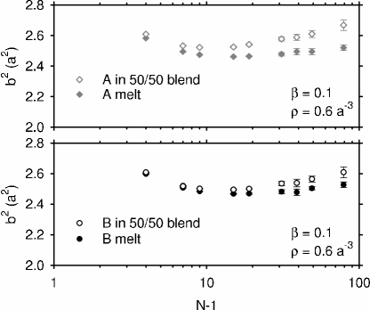
Figure 3: Simulation results for the squared effective bond lengths, $b^{2}=6R_{g}^{2}/(N-1)$, of polymer chains as a function of the number of bonds, $N-1$, for a 50/50 blend and for the A and B melts at the temperature and monomer density indicated in the figure. The upper and lower panels show the results for chains of type A and B, respectively. A comparison of the chain dimensions in the blends (open symbols) with those in the melts (filled symbols) shows that both types of chains are expanded in the blend.

The effective bond length, which is related to the radius of gyration through Eq. (14) depends on the structure as well as the environment of the chains. In Fig. 3 we present simulation results for the squared effective bond length as a function of chain length for A and B chains in the melt and in a blend with mass fraction $c_{A}=0.5$. We note, first of all, that for both melts and blends the bond length approaches a constant value for long chain lengths, as expected for Gaussian chains, see Eq. (14). Furthermore, the effective bond length of both A and B chains is larger in the blend than in the melt. At all densities, the chain expansion increases with increasing dilution, i.e. chains are most expanded when they are surrounded by chains of the other component. This is due to the relatively large attractive interaction energy associated with contacts between unlike monomers; the mixed interaction with energy $\epsilon_{AB}=-2\epsilon$ is twice as attractive as the interaction between A segments, $\epsilon_{AA}=-1\epsilon$, so that A monomers seek out B monomers as neighbors, which stretches the chains.

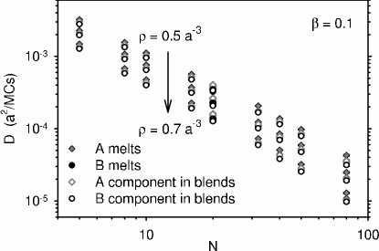
Figure 4: Self diffusion coefficients as a function of chain length for all melts and blends considered in this work. The filled and open symbols represent simulation results for melts and blends, respectively, while diamonds and circles stand for chains of type A and B, respectively. The results represent three different monomer densities, $\rho=0.5a^{-3}$, $\rho=0.6a^{-3}$, and $\rho=0.7a^{-3}$, and show the expected decrease of the self-diffusion coefficients with increasing density. In this graph, results for the B melts are hidden by the symbols for blend results.

Self diffusion coefficients give information about the large scale dynamics of melts and blends. They are determined from Monte Carlo simulations as described in Section III. In Fig. 4 we present results for the self-diffusion coefficients as a function of chain length for all melts and blends considered in this work. As expected, the self-diffusion coefficients decrease with increasing monomer density $\rho$ and chain length $N$. The chain-length dependence of the self-diffusion coefficients in Fig. 4 is intermediate between the scaling laws $D\sim N^{-1}$ and $D\sim N^{-2}$ expected from Rouse and reptation theory, respectively. This is expected since chain-end effects mask the Rouse behavior of short chains in dense systems (see e.g. Refs. Pearson et al., 1987, 1994) while fully entangled behavior is not usually seen for chains of the relatively short lengths simulated here Binder and Paul (1997); Müller et al. (2000); Tanaka et al. (2000); Kreer et al. (2001); Paul and Smith (2004); León et al. (2005). The graph also shows that the self-diffusion coefficients for A melts are typically larger than those for the blends. (The symbols for the B melts are hidden by the symbols for the blends.) The differences between the dynamics of the two components and the composition dependence of the self-diffusion coefficients will be discussed in detail for chains of length $N=20$ below.

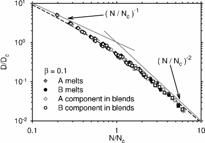
Figure 5: Scaling representation of the self-diffusion coefficients for all melts and blends considered in this work. The symbols, which are the same as in Fig. 4 represent values of the self-diffusion coefficient $D$ divided by $D_{\mathrm{c}}=\mu/N_{\mathrm{c}}$ calculated from Eqs. (5), (20), and (15) as a function of the chain length $N$ divided by the characteristic chain length $N_{\mathrm{c}}$ calculated from Eq. (15). The dashed line represents the crossover function of Hess Hess (1986, 1988), see Eq. (9), while the gray solid lines represent the limiting power laws of the Rouse and reptation models Doi and Edwards (1986), see Eq. (8).

In Fig. 5 we present the self-diffusion coefficient data of Fig. 4 in scaling form, $D/D_{\mathrm{c}}$ as a function of $N/N_{\mathrm{c}}$, where $D_{\mathrm{c}}$ is calculated from Eqs. (5), (20), and (15) and $N_{\mathrm{c}}$ is calculated from Eq. (15). In the graph, both melt and blend data for different chain lengths and densities collapse onto a common line. This suggests that scaling of dynamic properties with the packing length may be applicable to blends as well as melts. It also gives us some confidence in our construction of mobilities from the acceptance rates and the effective bond lengths ($\mu\sim b^{2}A_{\text{rate}}$). A comparison with the gray solid lines indicating the power laws expected from Rouse and reptation theory Doi and Edwards (1986) (Eq. 8) confirms that most of our data are in the crossover region between unentangled and fully entangled behavior. The dashed line in Fig. 5 represents the crossover equation (9) of Hess Hess (1986, 1988), which was used to determine values for the two constants $C_{\mu}$ and $C_{c}$ appearing in Eqs. (20) and (15). There is some uncertainty in the results for the constants since more than one combination of $C_{\mu}$ and $C_{c}$ values leads to a respectable representation of the data in the crossover region. However, a difference in a constant prefactor for the mobilities $\mu$ is of little concern since we are interested in the variation with density and composition rather than the absolute values of the mobilities and the corresponding friction coefficients $\zeta=1/\mu\beta$.

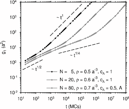
Figure 6: Average mean squared displacement $g_{1}$ of the innermost monomer as a function of time for chains of type A with three different reduced chain lengths $N/N_{\mathrm{c}}$. The symbols connected by thin solid lines represent, from top to bottom, results for chains of length $N=5$ in a melt of density $\rho=0.5a^{-3}$ ($N/N_{\mathrm{c}}=0.19$), chains of length $N=20$ in a melt of density $\rho=0.6a^{-3}$ ($N/N_{\mathrm{c}}=0.96$), and chains of length $N=80$ in a 50/50 blend of density $\rho=0.7a^{-3}$ ($N/N_{\mathrm{c}}=6.2$). The dashed lines indicate the power laws expected for $g_{1}(t)$ from reptation theory Doi and Edwards (1986).

To help interpret our values for the characteristic chain lengths $N_{\mathrm{c}}$ we present in Fig. 6 average mean-squared displacements of the central monomer, $g_{1}(t)$, for three systems corresponding to the smallest, the largest and an intermediate value of $N/N_{\mathrm{c}}$ in Fig. 5. The symbols connected by solid lines represent values calculated from Eq. (17) with the block algorithm. They represent results for an A-melt of chains of length $N=5$ at density $\rho=0.5a^{-3}$ with $N/N_{\mathrm{c}}=0.19$ (top), an A-melt of chains of length $N=20$ at density $\rho=0.6a^{-3}$ with $N/N_{\mathrm{c}}=0.96$ (center), and the A component in a 50/50 blend of chains of length $N=80$ at density $\rho=0.7a^{-3}$ with $N/N_{\mathrm{c}}=6.2$ (bottom). All three examples show the expected diffusive behavior ($g_{1}\sim t$) at long times. The behavior at short times is subdiffusive but not quite Rouse-like ($g_{1}\sim t^{1/2}$), as is generally observed in simulations Kreer et al. (2001); Paul (2002). The largest $g_{1}(t)$ values correspond to the smallest reduced chain length, $N/N_{\mathrm{c}}=0.19$, and illustrate unentangled behavior; the slope of $g_{1}(t)$ in this double logarithmic plot increases monotonically from the subdiffusive region at short times until it reaches a value of unity in the diffusive region, which starts around $10^{3}$ MCs for this system. The smallest $g_{1}(t)$ values correspond to the largest reduced chain length, $N/N_{\mathrm{c}}=6.2$. In this case, a second subdiffusive region at intermediate times is clearly visible. The slope in this region has a value of about 0.37 which is not as small as the value of $1/4$ expected for fully entangled chains from reptation theory Doi and Edwards (1986). This implies that even the longest chains in our simulations are not fully entangled. The line of intermediate $g_{1}(t)$ values in Fig. 6, finally, corresponds to a melt with chains near the characteristic chain length ($N/N_{\mathrm{c}}=0.96$). In this case, the slope of $g_{1}(t)$ decreases only slightly before it rises to the diffusive value of unity. This suggests that the chains are just starting to feel entanglement effects for reduced chain lengths near $N/N_{\mathrm{c}}\simeq 1$.

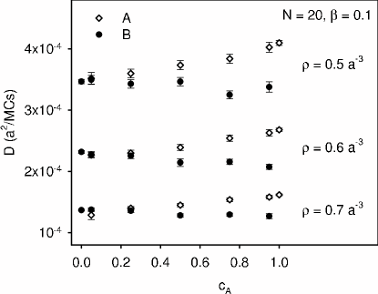
Figure 7: Self-diffusion coefficients of melts and blends as a function of blend composition for chains of length $N=20$ and monomer densities $\rho=0.5A^{-3}$ (top), $\rho=0.6A^{-3}$ (center), and $\rho=0.7A^{-3}$ (bottom). Results for A melts and the A component in blends are represented by open diamonds, while those for B melts and the B component in blends are represented by filled circles; $c_{A}$ denotes the mass fraction of component A.

In order to investigate the composition dependence of the dynamics, we focus in the following on one chain length, $N=20$, and investigate a broad range of compositions ranging from the pure melts ($c_{A}=0$, $c_{A}=1$) to the dilute limits ($c_{A}=0.05$, $c_{A}=0.95$) with three intermediate compositions ($c_{A}=0.25$, $c_{A}=0.5$, and $c_{A}=0.75$), for the three monomer densities, $\rho=0.5a^{-3}$, $\rho=0.6a^{-3}$, and $\rho=0.7a^{-3}$ and reduced inverse temperature $\beta=0.1$. In Fig. 7 we present the simulation results for the self-diffusion coefficients of the $N=20$ melts and blends as a function of composition for the three monomer densities $\rho=0.5a^{-3}$, $\rho=0.6a^{-3}$, and $\rho=0.7a^{-3}$. These results show that, in general, the composition dependence of the self-diffusion coefficients decreases with increasing density and is stronger for the A component than for the B component. The trends for the self-diffusion coefficients are the same at each density; as the mass fraction $c_{A}$ of the A component increases, the self-diffusion coefficients of A chains increase while those of B chains decrease. Hence, for both types of chains, blending tends to reduce the values of the self-diffusion coefficients from the melt values (the self-diffusion coefficients of the B components are largest in B melts and decrease as A component is added, while the $D$ values of A chains are largest in the A melt and decrease as B component is added to the blends). For most blends considered here, the self-diffusion coefficients of the A component are larger than those of the B component. This is true for all blends of the lowest density considered here, $\rho=0.5a^{-3}$. However, for the density $\rho=0.6a^{-3}$, the values of the self-diffusion coefficients of both components are comparable for blends with small A content. For the highest density considered in our simulations, $\rho=0.7a^{-3}$, finally, the self-diffusion coefficient of the A component is even smaller than that of the B component for the smallest blend value of $c_{A}$.

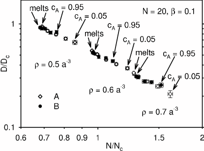
Figure 8: Scaling representation of the self-diffusion coefficients for melts and blends with chain length $N=20$ at the monomer densities $\rho=0.5a^{-3}$, $\rho=0.6a^{-3}$, and $\rho=0.7a^{-3}$. The open diamonds and filled circles correspond to results for the A and B component, respectively. For each density, the results for the pure melts correspond to the lowest reduced chain lengths $N/N_{\mathrm{c}}$ and the largest values of the scaled self-diffusion coefficients $D/D_{\mathrm{c}}$. Conversely, the largest values of $N/N_{\mathrm{c}}$ and the smallest values of $D/D_{\mathrm{c}}$ for each density correspond to the minority component in a dilute blend.

In Fig. 8 we present simulation results of the self-diffusion coefficients in scaled form, $D/D_{\mathrm{c}}$ as a function of $N/N_{\mathrm{c}}$. The data are a subset of those presented in Fig. 5 and belong to the crossover region near $N/N_{\mathrm{c}}=1$. In the double-logarithmic graph of Fig. 8, the reduced self-diffusion coefficient data follow closely a straight line with a slope of about -1.7. The reduced diffusion coefficients of the minority components in dilute blends appear to lie somewhat above this line; however, this may not be significant considering the uncertainty in the data. Hence, the data in Fig. 8 may be approximated by

$$D/D_{\mathrm{c}}\simeq\text{const.}\times(N/N_{\mathrm{c}})^{-\nu}\text{ with }\nu\simeq 1.7,$$ (22)

which implies

$$D\simeq\text{const.}\times\mu N_{\mathrm{c}}^{\nu-1}N^{-\nu},$$ (23)

where $D_{\mathrm{c}}=\mu/N_{\mathrm{c}}$ of Eq. (5) has been used. The results presented in Fig. 8 suggest that the scaling with a characteristic chain length $N_{\mathrm{c}}$ derived from the packing length and a characteristic diffusion coefficient $D_{\mathrm{c}}=\mu/N_{\mathrm{c}}$ constructed with the mobility $\mu\sim b^{2}A_{\text{rate}}$ captures both density and composition dependence of the self diffusion coefficients for these blends.

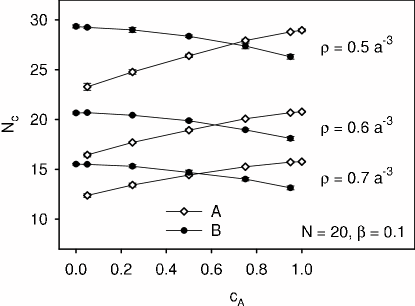
Figure 9: Scaling chain length $N_{\mathrm{c}}$ as a function of blend composition for melts and blends with chain length $N=20$ at the indicated densities. The symbols connected by solid lines represent values calculated from Eq. (15) with Eq. (14) for components A (open diamonds) and B (filled circles).

In order to gain insight into the origin of the variation of the self-diffusion coefficients with density and blend composition, we present in Figs. 9, 10, and 11 results for the characteristic chain lengths, the acceptance rates, and the mobilities of the melts and blends with $N=20$. The results for the scaling chain lengths $N_{\mathrm{c}}$ in Fig. 9 show that $N_{\mathrm{c}}$ increases with increasing density. This suggests a decrease of the entanglement length with increasing density, which is expected since the distance between monomers from different chains decreases with increasing density Milner (2005). The $N_{\mathrm{c}}$ values in Fig. 9 also show that blending decreases the characteristic chain length for the blends considered here; for both types of chain, the values of $N_{\mathrm{c}}$ decrease with increasing concentration of the other component at a given density. This composition dependence of $N_{\mathrm{c}}$ is a result of the variation of the effective bond length $b$ with composition. The results for $b^{2}$ in Fig. 14 show that both A and B chains are expanded in a blend compared to the melt. Since, according to Eq. (15), a larger effective bond length corresponds to a smaller characteristic chain length, the values of $N_{\mathrm{c}}$ decrease upon blending from their melt values.

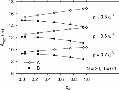
Figure 10: Average acceptance rates for elementary moves as a function of blend composition for melts and blends with chain length $N=20$ at the indicated densities. The open diamonds and filled circles connected by solid lines represent simulation results for components A and B, respectively.

The average acceptance rates for elementary moves of our Monte Carlo simulations presented in Fig. 10 measure the average probability for a monomer to complete an attempted move to a nearest-neighbor site. In the lattice model for polymer blends employed in this work, this probability depends, first of all, on the local bond structure since only three different bond lengths are allowed. It also depends strongly on the local density since the monomer cannot move to a site that is already occupied by another monomer. The composition of the blends affects the acceptance rate through the change in internal energy associated with a move. The internal energy of the system depends on the numbers ($N_{ij}$) and the interaction energies ($\epsilon_{ij}$, $i,j\in\{A,B\}$) of contacts between non-bonded nearest neighbors, see Eq. (10). According to the Metropolis criterion, a move is always accepted when the new configuration has a lower internal energy than the original one. If the new internal energy is higher, the move is accepted only with a probability corresponding to the Boltzmann factor of the energy difference between old and new configurations. This implies that the acceptance rate for moves is small, when the new site has a smaller number of occupied nearest neighbor sites or when the interactions with the new neighbors are less attractive than those with the old. Finally, a small fraction of moves is prohibited because it would lead to the crossing of bonds. The results for the acceptance rates in Fig. (10) show the expected strong dependence on the monomer density. In order to understand the composition dependence, we start by considering blends, where the A component is dilute, i.e. near $c_{A}=0$. In this case, the A chains are surrounded by B chains. Since the interaction energies for AB and BB contacts are identical, $\epsilon_{AB}=\epsilon_{BB}=-2\epsilon$, we expect similar acceptance rates for the A and B component at a given density. This is indeed what the data in Fig. 10 show. For all compositions and densities, the acceptance rates for the A component are higher than those of the B component. Furthermore, for a given density, as A component is added to a blend, the mobility of A monomers increases while that of B monomers decreases. There are two factors, both related to the energetics, that contribute to this. First of all, since A-A contacts are less attractive than A-B contacts ($\epsilon_{AA}=-1\epsilon$ while $\epsilon_{AB}=-2\epsilon$), A monomers become increasingly more mobile as A component is added to a blend. Secondly, the local density near A monomers is somewhat lower than that near B monomers leading to a larger mobility of A monomers. The reason for the local density variation is the difference in the average energy penalty for making a contact with a void instead of another monomer. For B monomers, this penalty is always $2\epsilon$. For A monomers, on the other hand, it varies with composition between $2\epsilon$ near $c_{A}=0$ and $1\epsilon$ near $c_{A}=1$. The effect becomes smaller with increasing monomer density since the number of voids decreases.

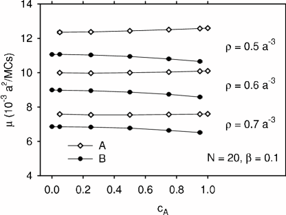
Figure 11: Mobility $\mu$ as a function of blend composition for melts and blends with chain length $N=20$ at the indicated densities. The symbols connected by solid lines represent values calculated from Eq. (20) with Eq. (14) for components A (open diamonds) and B (filled circles).

In Fig. 11 we present results for the composition dependence of the mobilities, calculated from Eq. (20) with Eq. (14), for the melts and blends with chain length $N=20$. The mobilities are proportional to both the acceptance rates and the squared effective bond lengths, $\mu\sim b^{2}A_{\text{rate}}$. It is not surprising that they show some of the characteristics of the acceptance rates discussed above. Just like the acceptance rate, the mobility decreases with increasing density. Furthermore, chains of type A always have a larger mobility than chains of type B, which makes A the faster component in the blend at all compositions. However, the composition dependence of the effective bond length partially compensates that of the acceptance rate and makes the mobilities less dependent on composition than the acceptance rates. As A component is added to a blend, the mobility of A chains increases, while that of B chains decreases only slightly. In the limit where the A component is dilute, the mobilities of the two components remain distinct, while the acceptance rates of the two components converge. Conversely, in the limit of dilute B in A, the relative differences between mobilities of the components are smaller than those of the acceptance rates.

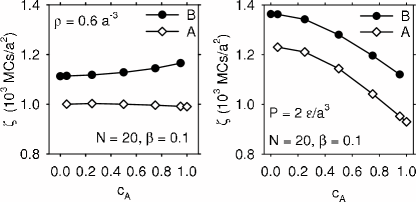
Figure 12: Local friction coefficients as a function of composition for melts and blends with chain length $N=20$. The symbols in the left panel represent values $\zeta=1/\beta\mu$ corresponding to the mobilities $\mu$ at the constant density $\rho=0.6a^{-3}$ in Fig. 11. The symbols in the right panel represent friction coefficient values interpolated from the data in Fig. 13 to a constant pressure of $P=2\epsilon/a^{3}$. The solid lines only connect the symbols.

The local friction coefficients $\zeta$ of the blend components are inversely proportional to the mobilities, $\zeta=1/\beta\mu$ (Eq. (21)). In the left panel of Fig. 12, we present values for the local friction coefficients calculated from the mobility results for melts and blends of density $\rho=0.6a^{-3}$ presented in Fig. 11. Since A is the faster component, its friction coefficients are smaller than those of the B component. As the mass fraction of A chains increases, the friction coefficients of the A component decrease (slightly) while those of the B component increase. Hence, when A component is added to a blend at constant density, A segments speed up (somewhat) while B segments slow down. This is the case for all densities considered here and contrasts with the experimental observation that both components speed up when the fraction of faster component in a blend is increased. The reason for this apparent discrepancy is that we have varied the composition at constant density $\rho$, whereas in experiments the composition is typically varied at constant pressure. In order to arrive at friction coefficient values at constant pressure, we first consider their pressure dependence and then interpolate our data to a given pressure. In this work, we estimate the pressure using a random mixing approximation for the internal energy and the Flory-Huggins expression for the entropic contribution Flory (1953). This is expected to yield at least qualitatively correct results since our simulations are carried out at high density, where the Flory-Huggins theory has been found to give a reasonable representation of the pressure of athermal lattice chains Dickman and Hall (1986); Dickman (1987), and since we work at a constant, high temperature where the random mixing approximation is expected to be adequate. In Fig. 13 we present results for the friction coefficients of melts and blends with $N=20$ as a function of pressure. As expected, the friction coefficients increase with increasing pressure for each composition. In this representation it becomes apparent that the friction coefficients of both components decrease when the mass fraction of A is increased at constant pressure. To illustrate this further, we have estimated values for friction coefficients at the pressure $P=2\epsilon/a^{3}$ by interpolation of the results in Fig. 13. These values are presented as a function of mass fraction in the right panel of Fig. 12. In qualitative agreement with experiment, the results for the friction coefficients show that the dynamics of both components speed up when the fraction of the fast component (A) is increased at constant pressure.

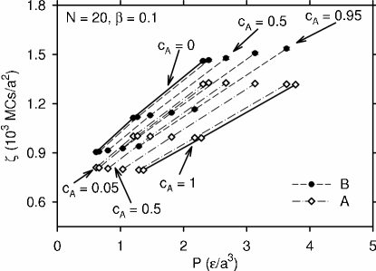
Figure 13: Local friction coefficients as a function of pressure for melts and blends with chain length $N=20$. The symbols represent values of $\zeta=1/\beta\mu$ corresponding to the mobilities $\mu$ in Fig. 11. The pressure has been estimated from Flory-Huggins theory Flory (1953). The dashed and dashed-dotted lines connect values for the B and A components, respectively, in blends of a given composition; melt values are connected by solid lines. The results shown here correspond to mass fractions $c_{A}=0$, 0.05, 0.25, 0.5, 0.75, 0.95, and 1.0. The friction coefficients for the B component in the melt and in the blend with $c_{A}=0.05$ are too close to be distinguished in this representation.

V Discussion

In this work, we have presented Monte Carlo simulation results for polymer melts and blends with a range of densities, compositions and chain lengths. In order to represent the two components of a binary blend, we have generalized Shaffer’s bond fluctuation model for athermal melts Shaffer (1994, 1995); Pan and Shaffer (1996) by introducing attractive interactions between occupied non-bonded nearest neighbor sites on the lattice. The interactions parameters employed in this work are $\epsilon_{AA}=-1\epsilon$ and $\epsilon_{BB}=-2\epsilon$ for like interactions between monomers of type A and B, respectively, and $\epsilon_{AB}=-2\epsilon$ for interactions between unlike monomers. All simulations were carried out a fixed temperature of $T=10\epsilon/k_{\mathrm{B}}$ corresponding to an inverse reduced temperature of $\beta=0.1$. Our results for the effective bond length presented in Fig. 3 show that the chain dimensions of both types of chains increase upon blending. This effect increases with increasing dilution and is due to the large attractive interaction energy associated with contacts between unlike monomers.

Self-diffusion coefficients were determined from the mean square displacement of the center of mass of the chains. The simulation results presented in Fig. 4 show that the chain-length dependence of the self-diffusion coefficients falls between the power laws expected from Rouse and reptation theory Doi and Edwards (1986), which is expected for the range of chain lengths considered in this work Binder and Paul (1997); Müller et al. (2000); Tanaka et al. (2000); Kreer et al. (2001); Paul and Smith (2004); León et al. (2005). In order to investigate the scaling behavior of the self-diffusion coefficients, characteristic chain lengths $N_{\mathrm{c}}$ were calculated from the packing lengths of the chains. Segmental mobilities $\mu$ were determined from the acceptance rates and the effective bond lengths and combined with the values for $N_{\mathrm{c}}$ to yield characteristic self-diffusion coefficients $D_{\mathrm{c}}=\mu/N_{\mathrm{c}}$. The results for the reduced diffusion coefficients $D/D_{\mathrm{c}}$ as a function of the reduced chain length $N/N_{\mathrm{c}}$ presented in Figs. 5 and Figs. 8 show the data for melts and blends with different chain lengths, densities, and compositions to collapse onto a common line. This suggests that the scaling of dynamic properties with the packing length, which has been observed for polymer melts Lin (1987); Kavassalis and Noolandi (1987); Fetters et al. (1999); Everaers et al. (2004); Sukumaran et al. (2005); Milner (2005), may be applicable to blends as well.

The composition dependence of the dynamic properties was studied in detail for chains of length $N=20$ in melts and blends of three different densities. The results for the self diffusion coefficients $D$ presented in Fig. 7 show the expected variation with density. At each density and for both types of chains, blending reduces the self-diffusion coefficient from its melt value. This may be attributed to the composition dependence of the mobility $\mu$ and the characteristic chain length $N_{\mathrm{c}}$, as follows. The scaling representation of Fig. 8 for chains of length $N=20$ shows that the reduced self-diffusion coefficient follow approximately a power law with exponent $\nu=1.7$. This implies that $D$ depends on the mobility $\mu$ and the characteristic chain length $N_{\mathrm{c}}$ approximately as $D=\text{const.}\times\mu N_{\mathrm{c}}^{\nu-1}N^{-\nu}$, see Eq. (23). Since the values of both the mobility and the characteristic chain length decrease upon blending, so do the values of the self-diffusion coefficients.

The variation of the self-diffusion coefficients with composition has another interesting aspect. For the highest density, $\rho=0.7a^{-3}$ the difference between the self-diffusion coefficients of the two components changes sign from $D_{A}-D_{B}<0$ to $D_{A}-D_{B}>0$ at a mass fraction of A of about $c_{A}\simeq 0.2$. This is surprising since it implies that, for $\rho=0.7a^{-3}$, A chains move more slowly than B chains at low A concentrations but faster than B chains at higher A concentrations. Since changes in both mobility and characteristic chain length affect the value of the diffusion coefficient we consider them in turn. Results for the segmental mobility presented in Fig. 11 show that the local mobility of the A chains in a blend is always larger than that of the B chains. This implies that, on the length scale of an effective bond, the A component is always the fast component in the blends considered here. Hence, the segmental mobility cannot be responsible for the sign change of $D_{A}-D_{B}$. Results for the characteristic chain lengths $N_{\mathrm{c}}$ in Fig. 9 show that, for all densities, the differences between the characteristic chain lengths change sign from $N_{cA}-N_{cB}<0$ to $N_{cA}-N_{cB}>0$ at intermediate mass fractions. This, together with the relatively weak composition dependence of the mobility at $\rho=0.7a^{-3}$, gives rise to the sign change of $D_{A}-D_{B}$. In physical terms; for the highest density considered here and at the lowest concentration of A chains, the characteristic chain length for A chains is so much smaller than that of B chains, that entanglement effects lead to A chains diffusing more slowly than B chains even though the segmental mobility of the A chains is larger than that of the B chains.

Values for the local friction coefficients $\zeta$ have been determined from the results for the segmental mobilities $\mu$. The pressure dependence of the friction coefficients is shown in Fig. 13, where the values for the pressure are estimated from the Flory-Huggins theory Flory (1953). The results show the expected increase in the friction coefficients with increasing pressure. The pressure dependence is slightly larger for the slower (B) component than for the faster (A) component, which agrees qualitatively with results from our calculations for polyolefin blends Luettmer-Strathmann (2005). In Fig. 12, we contrast two sets of results for the composition dependence of the local friction coefficients. The results in the left panel, where the composition of the blends is varied at constant density, as is typical for simulations, are qualitatively different from those in the right panel, where the pressure is kept approximately constant, as is typical for experiments. The results for the constant-pressure composition dependence of the friction coefficients agree qualitatively with experimental observations on miscible blends; the friction coefficients of both components decrease with increasing mass fraction of the fast component (A).

In this work, we calculate the local friction coefficients from the mobility $\mu$, which describes the dynamics on the scale of the effective bond length. For polymer melts near the glass transition Inoue and Osaki (1996) and for miscible polyolefin blends Neelakantan et al. (2005), the Kuhn length has been identified as the size of the moving segment relevant to local dynamics. For the blend model considered here, the effective bond length and the Kuhn length are comparable in size, which makes it difficult to distinguish between these choices for the size of the moving segments. However, we hope that a current investigation of the dynamics of athermal melts for a larger set of densities will give us some insight into this question Luettmer-Strathmann and Khatri .

It is encouraging that these first simulation results for our lattice model for polymer blends reproduce trends observed in experimental work on polymer blends. The differences between the friction coefficients of the two melts and between the melts and the blends, however, are fairly small. The reason is that chains of type A and B differ only in the values of the interaction parameters and that the simulations are carried out at high temperature. In real polymer blends, the blend components typically differ in chain stiffness, which is known to have a large effect on the dynamics Fetters et al. (1999); Milner (2005); Müller et al. (2000); Kamath et al. (2003). In order to simulate more realistic systems and to increase the difference between the chains of the blend components, we are currently extending our model to include a differences in chain stiffness.

References

- Doi and Edwards (1986) M. Doi and S. F. Edwards, The Theory of Polymer Dynamics (Clarendon, Oxford, 1986).
- Grosberg and Khokhlov (1994) A. Y. Grosberg and A. R. Khokhlov, Statistical Physics of Macromolecules, AIP Series in Polymers and Complex Materials (American Institute of Physics, Woodbury, NY, 1994).
- de Gennes (1979) P.-G. de Gennes, Scaling Concepts in Polymer Physics (Cornell University, Ithaca, NY, 1979).
- Ferry (1980) J. D. Ferry, Viscoelastic Properties of Polymers (Wiley, New York, 1980), 3rd ed.
- Roland and Ngai (1991) C. M. Roland and K. L. Ngai, Macromolecules 24, 2261 (1991).
- Roland and Ngai (1992) C. M. Roland and K. L. Ngai, Macromolecules 25, 363 (1992), Macromolecules 33, 3184 (2000).
- Chung et al. (1994a) G. C. Chung, J. A. Kornfield, and S. D. Smith, Macromolecules 27, 964 (1994a).
- He et al. (2003) Y. He, T. R. Lutz, and M. D. Ediger, J. Chem. Phys. 119, 9956 (2003).
- Chung et al. (1994b) G. C. Chung, J. A. Kornfield, and S. D. Smith, Macromolecules 27, 5729 (1994b).
- Alégria et al. (1994) A. Alégria, J. Colmenero, K. L. Ngai, and C. M. Roland, Macromolecules 27, 4486 (1994).
- Kim et al. (1995) E. Kim, E. J. Kramer, and J. O. Osby, Macromolecules 28, 1979 (1995).
- Pathak (2001) J. A. Pathak, Ph.D. thesis, The Pennsylvania State University (2001).
- Min et al. (2001) B. Min, X. H. Qiu, M. D. Ediger, M. Pitsikalis, and N. Hadjichristidis, Macromolecules 34, 4466 (2001).
- Haley et al. (2003) J. C. Haley, T. P. Lodge, Y. He, M. D. Ediger, E. D. von Meerwall, and J. Mijovic, Macromolecules 36, 6142 (2003).
- Lutz et al. (2003) T. R. Lutz, Y. He, M. D. Ediger, H. Cao, G. Lin, and A. A. Jones, Macromolecules 36, 1724 (2003).
- Haley and Lodge (2004) J. C. Haley and T. P. Lodge, Colloid Polym. Sci. 282, 793 (2004).
- Lutz et al. (2004) T. R. Lutz, Y. He, M. D. Ediger, M. Pitsikalis, and N. Hadjichristidis, Macromolecules 37, 6440 (2004).
- Alegría et al. (2002) A. Alegría, D. Gómez, and J. Colmenero, Macromolecules 35, 2030 (2002).
- Doxastakis et al. (2000) M. Doxastakis, M. Kitsiou, G. Fytas, D. N. Theodorou, N. Hadjichristis, G. Meier, and B. Frick, J. Chem. Phys. 112, 8687 (2000).
- Genix et al. (2005) A.-C. Genix, A. Arbe, F. Alvarez, J. Colmenero, L. Willner, and D. Richter, Phys. Rev. E 72, 031808 (2005).
- Kopf et al. (1997) A. Kopf, B. Dünweg, and W. Paul, J. Chem. Phys. 107, 6945 (1997).
- Kamath et al. (2003) S. Kamath, R. H. Colby, and S. K. Kumar, Macromolecules 36, 8567 (2003).
- Budzien et al. (2002) J. Budzien, C. Raphael, M. D. Ediger, and J. J. de Pablo, J. Chem. Phys. 116, 8209 (2002).
- Faller (2004) R. Faller, Macromolecules 37, 1095 (2004).
- Neelakantan et al. (2005) A. Neelakantan, A. May, and J. K. Maranas, Macromolecules 38, 6598 (2005).
- Zetsche and Fischer (1994) A. Zetsche and E. W. Fischer, Acta Polymerica 45, 168 (1994).
- Katana et al. (1995) G. Katana, E. W. Fischer, T. Hack, V. Abetz, and F. Kremer, Macromolecules 28, 2714 (1995).
- Kumar et al. (1996) S. K. Kumar, R. H. Colby, S. H. Anastasiadis, and G. Fytas, J. Chem. Phys. 105, 3777 (1996).
- Kamath et al. (1999) S. Kamath, R. H. Colby, S. K. Kumar, K. Karatasos, G. Floudas, G. Fytas, and J. E. L. Roovers, J. Chem. Phys. 111, 6121 (1999).
- Lodge and McLeish (2000) T. P. Lodge and T. C. B. McLeish, Macromolecules 33, 5278 (2000).
- Leroy et al. (2003) E. Leroy, A. Alegría, and J. Colmenero, Macromolecules 36, 7280 (2003).
- Kant et al. (2003) R. Kant, S. K. Kumar, and R. H. Colby, Macromolecules 36, 10087 (2003).
- Ngai and Roland (2004) K. L. Ngai and C. M. Roland, Rubber Chem. Technol. 77, 579 (2004).
- Luettmer-Strathmann (2005) J. Luettmer-Strathmann, J. Chem. Phys. 123, 014910 (2005).
- Graessley and Edwards (1981) W. W. Graessley and S. F. Edwards, Polymer 22, 1329 (1981).
- Lin (1987) Y.-H. Lin, Macromolecules 20, 3080 (1987).
- Kavassalis and Noolandi (1987) T. A. Kavassalis and J. Noolandi, Phys. Rev. Lett. 59, 2674 (1987).
- Fetters et al. (1999) L. J. Fetters, D. J. Lohse, S. T. Milner, and W. W. Graessley, Macromolecules 32, 6847 (1999).
- Everaers et al. (2004) R. Everaers, S. K. Sukumaran, G. S. Grest, C. Svaneborg, A. Sivasubramanian, and K. Kremer, Science 303, 823 (2004).
- Sukumaran et al. (2005) S. K. Sukumaran, G. S. Grest, K. Kremer, and R. Everaers, J. Polym. Sci. Part B: Polym. Phys. 43, 917 (2005).
- Milner (2005) S. T. Milner, Macromolecules 38, 4929 (2005).
- Binder and Paul (1997) K. Binder and W. Paul, J. Polym. Sci. B: Polym. Phys. 35, 1 (1997).
- Müller et al. (2000) M. Müller, J. P. Wittmer, and J.-L. Barrat, Europhys. Lett. 52, 406 (2000).
- Tanaka et al. (2000) M. Tanaka, K. Iwata, and N. Kuzuu, Comput. Theor. Polym. Sci. 10, 299 (2000).
- Kreer et al. (2001) T. Kreer, J. Baschnagel, M. Müller, and K. Binder, Macromolecules 34, 1105 (2001).
- Paul and Smith (2004) W. Paul and G. D. Smith, Rep. Prog. Phys. 67, 1117 (2004).
- León et al. (2005) S. León, N. van der Vegt, L. Delle Site, and K. Kremer, Macromolecules 38, 8078 (2005).
- Hess (1986) W. Hess, Macromolecules 19, 1395 (1986).
- Hess (1988) W. Hess, Macromolecules 21, 2620 (1988).
- Paul et al. (1991) W. Paul, K. Binder, D. W. Heermann, and K. Kremer, J. Phys. II 1, 37 (1991).
- Shaffer (1994) J. S. Shaffer, J. Chem. Phys. 101, 4205 (1994).
- Shaffer (1995) J. S. Shaffer, J. Chem. Phys. 103, 761 (1995).
- Pan and Shaffer (1996) X. Pan and J. S. Shaffer, Macromolecules 29, 4453 (1996).
- Newman and Barkema (1999) M. E. J. Newman and G. T. Barkema, Monte Carlo methods in statistical physics (Clarendon Press, Oxford, UK, 1999).
- Frenkel and Smit (1996) D. Frenkel and B. Smit, Understanding Molecular Simulations - From Algorithms to Applications (Academic Press, San Diego, CA, 1996).
- Paul (2002) W. Paul, Chemical Physics 284, 59 (2002).
- McCormick et al. (2005) J. A. McCormick, C. K. Hall, and S. A. Khan, J. Chem. Phys. 122, 114902 (2005).
- Pearson et al. (1987) D. S. Pearson, G. Ver Strate, E. von Meerwall, and F. C. Schilling, Macromolecules 20, 1133 (1987).
- Pearson et al. (1994) D. S. Pearson, L. J. Fetters, W. W. Graessley, G. Ver Strate, and E. von Meerwall, Macromolecules 27, 711 (1994).
- Flory (1953) P. J. Flory, Principles of Polymer Chemistry (Cornell University, Ithaca, NY, 1953).
- Dickman and Hall (1986) R. Dickman and C. K. Hall, J. Chem. Phys. 85, 3023 (1986).
- Dickman (1987) R. Dickman, J. Chem. Phys. 87, 2246 (1987).
- Inoue and Osaki (1996) T. Inoue and K. Osaki, Macromolecules 29, 1595 (1996).
- (64) J. Luettmer-Strathmann and R. Khatri, in preparation.