Interacting electrons on a quantum ring: exact and variational approach

Abstract

We study a system of interacting electrons on a one-dimensional quantum ring using exact diagonalization and the variational quantum Monte Carlo method. We examine the accuracy of the Slater-Jastrow -type many-body wave function and compare energies and pair distribution functions obtained from the two approaches. Our results show that this wave function captures most correlation effects. We then study the smooth transition to a regime where the electrons localize in the rotating frame, which for the ultrathin quantum ring system happens at quite high electron density.

1 Introduction

Various low-dimensional electron systems have been the subject of considerable scientific interest for more than two decades. Examples of these structures can be formed in a two-dimensional electron gas by applying appropriate confinement, thus restricting the motion of electrons to a small area on the boundary between two semiconducting materials. These systems are in many ways similar to atoms, however, their properties can be controlled by adjusting their geometry, the external confinement, and applied magnetic field. Nanostructures are a source of discoveries of novel quantum phenomena which do not appear in atoms. They are important both in connection with potential device applications and can function as convenient samples to probe the properties of many-electron systems in reduced dimensions.

In quantum rings, electrons are confined to move on a circular region in space. They have many interesting and actively explored properties: Under the influence of a magnetic field, an equilibrium current flows along the ring. Furthermore, the energy spectrum is periodic in the magnetic flux with a period of the flux quantum $\Phi_{0}=h/e$ in case of an even number of noninteracting electrons, but $\Phi_{0}/2$ for an odd number. Recently, the existence of a fractional periodicity has been discovered both in experiments [1] as well as in theoretical and computational studies [2, 3, 4, 5, 6, 7, 8]. This is often referred to as the fractional Aharonov-Bohm effect.

In this paper we study the accuracy of a variational quantum Monte Carlo (VMC) approach, using the Jastrow-Slater wave function, to quantum ring systems. This approach has been found to be extremely accurate in the case of quantum dots [9]. The main advantages of quantum Monte Carlo (QMC) methods are their applicability to large electron systems and their accuracy in capturing electron-electron correlation effects. To date, very few QMC studies of the electronic properties of nanoscale semiconductor quantum rings have been done. Emperador et alinvestigated the fractional Aharonov-Bohm effect in few-electron quantum rings using multi-configurational diffusion Monte Carlo [7] and Borrmann and Harting used path integral Monte Carlo to study the transition between spin ordered and disordered Wigner crystal rings [10]. We are not aware of VMC calculations for the quantum rings, and due to this, even the accuracy of the Jastrow-Slater wave function is an interesting open question. On the other hand, the good performance of VMC on two-dimensional quantum dots makes it an appealing technique to study also systems that are closer to being one dimensional [11, 12]. As an ultimate test for VMC in this direction, we consider here the limit of a purely one-dimensional system.

We calculate using VMC the total energy and pair distribution function of the quantum ring, in zero magnetic field, containing up to six interacting electrons. The interaction is taken to be Coulombic. To test the accuracy of our approach we perform exact diagonalization (ED) calculations and compare the results. We will show that VMC gives a very accurate estimate of the ground state energy for all the cases studied here. In addition, the charge part of electron correlations is recovered in very satisfactory fashion. The only weak point of VMC is that the antiferromagnetic nature of the system seen in the exact treatment is not present in the VMC results. This shows that even though the simple VMC wave function is adequate for the charge part, the spin structure of the Jastrow-Slater wave function is not correct. On the other hand, the spin part has only a minor role in, e.g., the total energy.

Already at a moderate strength of interaction, the few-electron quantum ring shows a separation of spin and charge degrees of freedom. The spin Hamiltonian is well described by the antiferromagnetic Heisenberg model with exchange coupling $J$ [13], which is very small compared to the energy of orbital motion. We compare our results to the relations for $J$ derived by Fogler and Pivovarov [14] and show that they are in good agreement. We discuss the localization of electrons in relative coordinates and find a smooth transition starting already at $1<r_{s}<2$.

This paper is divided as follows. In section II we discuss our model of the quantum ring system and go in considerable detail through the two methods used to calculate its ground state properties, ED and VMC. Then the results are presented in Section III. Our conclusions follow in Section IV.

2 Model and methods

2.1 Model

We model the semiconductor quantum rings in the effective mass approximation by a many-body Hamiltonian

$$\mathcal{H}=-\frac{\hbar^{2}}{2m^{*}}\sum_{i=1}^{N}\frac{\partial^{2}}{\partial\theta_{i}^{2}}+\sum_{i<j}^{N}V(\theta_{ij})\ ,$$ (1)

where $\theta_{i}$ is the angular coordinate of the $i$th electron and $V(\theta_{ij})$ is the interaction potential between each pair of electrons. We assume that the ring is extremely narrow so that the electrons can only move at a certain radius, leading to a purely one-dimensional ring. The Coulomb interaction for a ring system is written as

$$V(\theta_{ij})=\frac{V_{C}}{R\sqrt{4\sin^{2}\left(\theta_{ij}/2\right)+\mu^{2}}}\ ,$$ (2)

where $R$ is the radius of the ring, $V_{C}$ controls the strength of the interaction, and $\mu$ is a small parameter that eliminates the singularity at $\theta_{ij}=0$. As the interaction between particles at the same position on the ring is $V_{C}/\mu R$, one can think the regularization of the potential to give the ring a width of $\mu R$.

The single-particle eigenstates of the noninteracting case are plane waves

$$\psi_{l}(\theta)=\exp(-\mathrm{i}l\theta)/\sqrt{2\pi R}\ ,$$ (3)

with energies

$$\varepsilon_{l}=\frac{\hbar^{2}}{2m^{*}R^{2}}l^{2}\ ,$$ (4)

where $l=0,\pm 1,\pm 2,\dots$ is the angular momentum quantum number. We scale the units so that the energy is measured in units of $E_{0}=h^{2}/(2m^{*}\pi^{2}R^{2})$ and length in units of $R$. The only parameter which is tuned is the interaction strength, and for the Coulomb interaction this can be translated into a change of the ring radius by the formula

$$V_{C}=\frac{R}{2a_{B}^{*}}\ ,$$ (5)

where $a_{B}^{*}$ is the effective Bohr radius. The results presented in this paper are for interaction strength in the range of 1 to 10, which corresponds to a radius of 21 nm to 209 nm assuming GaAs material parameters. For comparison, the quantum ring system studied by Keyser et al[1, 15] had a radius of around 150 nm, which corresponds to an interaction strength of $V_{C}=7.2$ in our units. The width of their ring can be estimated to be around 20 nm, which is in reasonable agreement with the value of $\mu=0.1$ used in this work.

In the following, we will occasionally use the one-dimensional $r_{s}$-parameter, which is the average distance between electrons. In our model, it is directly proportional to the radius of the ring and thus also to $V_{C}$

$$\frac{r_{s}}{a_{B}^{*}}=\frac{2\pi V_{C}}{N}\ .$$ (6)

2.2 Exact diagonalization

The exact diagonalization method (ED), originally called configuration interaction, is a systematic scheme to expand the many-particle wave function using the noninteracting states as a basis. This method traces back to the early days of quantum mechanics, to the work of Hylleraas [16]. The calculation of matrix elements for the many-body case was originally derived by Slater and Condon [17, 18, 19], and developed further by Löwdin [20]. The use of the term ED for this can be seen as an attempt to replace the term configuration interaction with a normal mathematical term [21]. This term might in some cases be misleading, as truly exact results are obtained only in the limit of an infinite basis.

As a simple example to start from, consider a single-particle Hamiltonian split into two parts $\mathcal{H}=\mathcal{H}_{0}+\mathcal{H}_{I}$, where the Schrödinger equation of the first part is solvable:

$$\mathcal{H}_{0}\phi_{i}(\mathbf{r})=\varepsilon_{i}\phi_{i}(\mathbf{r})\ ,$$ (7)

and the wave functions $\phi_{i}(\mathbf{r})$ form a orthonormal basis. The solution of the full Schrödinger equation can be expanded in this basis as $\psi(\mathbf{r})=\sum_{i}\alpha_{i}\phi_{i}(\mathbf{r})$. Inserting this into the Schrödinger equation

$$\mathcal{H}\psi(\mathbf{r})=E\psi(\mathbf{r})\ ,$$ (8)

results in

$$(\mathcal{H}_{0}+\mathcal{H}_{I})\sum_{i}\alpha_{i}\phi_{i}(\mathbf{r})=E\sum_{i}\alpha_{i}\phi_{i}(\mathbf{r})\ .$$ (9)

Using (7), multiplying with $\phi_{j}^{*}$ and integrating gives

$$\sum_{i}\alpha_{i}\varepsilon_{i}\delta_{ij}+\sum_{i}\alpha_{i}\int\phi_{j}^{*}(\mathbf{r})\mathcal{H}_{I}\phi_{i}(\mathbf{r})\rmd\mathbf{r}=E\sum_{i}\alpha_{i}\delta_{ij}$$ (10)

for every $j$. This can be written as a matrix equation

$$(H_{0}+H_{I})\mbox{\boldmath$\alpha$}=E\mbox{\boldmath$\alpha$}\ ,$$ (11)

where $H_{0}$ is a diagonal matrix whose $i$th element is $\varepsilon_{i}$, and the $ji$th element of $H_{I}$ is $\int\phi_{j}^{*}(\mathbf{r})\mathcal{H}_{I}\phi_{i}(\mathbf{r})\rmd\mathbf{r}$. The vector $\alpha$ contains the values $\alpha_{i}$. In this way, the Schrödinger equation can be mapped to a matrix form. In principle, the basis $\{\phi_{i}\}$ is infinite, but the calculations are done in a finite basis. The main computational task is to calculate the matrix elements of $H_{I}$ and to diagonalize the matrices. The convergence of the expansion depends on the actual values of the matrix elements, and in the case where $\mathcal{H}_{I}$ is only a small perturbation to $\mathcal{H}_{0}$ it is fastest.

In a similar fashion, one can split the many-particle Hamiltonian into two parts, typically a noninteracting and an interacting one. The solution to the noninteracting many-Fermion problem is a Slater determinant formed from the $N$ lowest energy eigenstates of the single-particle Hamiltonian. The basis typically chosen for the interacting problem is a Slater determinant basis constructed from $M$ single-particle states. For an $N$-particle problem, $M\choose N$ different many-particle configurations can be constructed by occupying any $N$ of the $M$ available states. Each of these determinants is labeled by the $N$ indices of the occupied single-particle states. Due to interactions, other configurations than the one of the noninteracting ground state have a finite weight in the expansion of the many-particle wave function.

The Schrödinger equation maps to matrix form in a similar way as in the preliminary example above. The calculation of the matrix elements of the Hamiltonian are simpler using second quantization and the occupation number representation. We will only state the results here.

The noninteracting Hamiltonian matrix $H_{0}$ in the determinant basis is diagonal with the $i$th element equal to $E_{i}=\sum_{j=1}^{N}\varepsilon_{i_{j}}$, where $i_{j}$ labels the occupied single-particle state. The elements of the interaction Hamiltonian matrix can be found by a straight-forward calculation using the anti-commutation rules of the creation and annihilation operators. The only non-zero matrix elements are between configurations that differ at most by two single-particle occupations. If both of the two configurations have two single-particle states occupied that are unoccupied in the other one, the interaction matrix element is

$$\pm(V_{pqrs}-V_{pqsr})\ ,$$ (12)

where $p$ and $q$ are single-particle states occupied in the left configuration and unoccupied in the right one, and similarly for $s$ and $r$ with right and left interchanged. The sign of the matrix element depends on the total number of occupations between $p$ and $r$ and between $q$ and $s$ due to anti-commutation of the creation and annihilation operators. If this number is odd, the sign is minus, otherwise plus. For the Coulomb interaction

$$V_{ijkl}=\delta_{s_{i},s_{k}}\delta_{s_{j},s_{l}}\int\phi_{i}^{*}(\mathbf{r}_{1})\phi_{j}^{*}(\mathbf{r}_{2})\frac{1}{r_{12}}\phi_{k}(\mathbf{r}_{1})\phi_{l}(\mathbf{r}_{2})\rmd\mathbf{r}_{1}\rmd\mathbf{r}_{2}\ ,$$ (13)

and the delta functions result from the spin part summation. In the case of a one-dimensional quantum ring this matrix element has a closed form

$$V_{ijkl}=\pi^{-1}Q_{i-k-\frac{1}{2}}\left(\mu^{2}/2+1\right)\ ,$$ (14)

where $Q(x)$ is the Legendre function which can be written in terms of Gauss’s hypergeometric function.

If the two configurations have a difference of only one occupation, the final result for the interaction matrix elements is

$$\pm\sum_{i}(V_{qiri}-V_{qiir})\ ,$$ (15)

where $q$ is occupied in the left configuration and unoccupied in the right one, and for $r$ the other way around. The sum over $i$ is over orbitals that are occupied in both configurations. Again the sign of the matrix element depends on number of occupations between the differing orbitals. It is easy to see that the matrix elements in (15) vanish for a rotationally symmetric system, as a change in only one occupation cannot conserve the total angular momentum.

The diagonal elements of the interaction Hamiltonian matrix are simply

$$\sum_{i<j}^{N}(V_{ijij}-V_{ijji})\ .$$ (16)

To summarize, the noninteracting part results in a Hamiltonian matrix which is diagonal, and the interaction Hamiltonian couples configurations that differ by at most two occupations. Now that we know the Hamiltonian matrix elements, we can sketch the basic ED procedure as follows: First solve for $M$ eigenstates of the single-particle Hamiltonian $\mathcal{H}_{0}$. After those have been found, calculate the two-particle matrix elements $V_{ijkl}$ of (13). Construct the $M\choose N$ $N$-particle configurations from $M$ single-particle states. Here configurations with wrong symmetry can be rejected. For example, one can pick only configurations with certain $z$-component of the total spin or some other good quantum number, like the angular momentum in our case. To construct the Hamiltonian matrix, calculate the interaction matrix elements of the Hamiltonian $\mathcal{H}_{I}$ between the configurations. Construct the diagonal noninteracting Hamiltonian matrix elements from the single-particle eigenvalues. Finally, diagonalize the Hamiltonian matrix. The main problem of the ED method is the exponential computational scaling of the method as a function of the number of particles. An other problem is the convergence rate as a function of basis size.

To compare the ED and VMC methods for the ring, we study the total energy and the pair distribution function of the electrons in the ring. The pair distribution function of the system is defined by

$$n_{\sigma}({\bf r})n_{\sigma^{\prime}}({\bf r}^{\prime})g_{\sigma\sigma^{\prime}}({\bf r},{\bf r}^{\prime})=\left<\psi\right|\Psi_{\sigma}^{\dagger}({\bf r})\Psi_{\sigma^{\prime}}^{\dagger}({\bf r}^{\prime})\Psi_{\sigma^{\prime}}({\bf r}^{\prime})\Psi_{\sigma}({\bf r})\left|\psi\right>\ ,$$ (17)

where $n_{\sigma}({\bf r})$ is the spin $\sigma$ particle density and $\Psi_{\sigma}^{\dagger}({\bf r})$ and $\Psi_{\sigma}({\bf r})$ are the field operators. It describes the probability that, given an electron of spin $\sigma$ at ${\bf r}$, an electron of spin $\sigma^{\prime}$ is found at ${\bf r}^{\prime}$. It therefore gives an idea of the strength of correlation between electrons. The pair distribution function can be derived in a similar way as the Coulomb matrix elements using the anti-commutation rules of the creation and annihilation operators.

2.3 Variational Monte Carlo method

The QMC methods are among the most accurate ones for tackling a problem of interacting quantum particles [22]. Often the simplest QMC method, namely, the variational QMC (VMC), is able to reveal the most important correlation effects. In many quantum systems, further accuracy in, e.g., the energy is needed, and in these cases methods such as the diffusion QMC allow one to obtain more accurate estimates for various observables.

The VMC strategy of solving the ground state of an interacting system of $N$ particles (defined by the Hamiltonian operator $\mathcal{H}$ and the particle statistics) starts by constructing the variational many-body wave function $\Psi$. Then, all the observables of the system can be computed from it. For example, the energy $E$, which is higher than the ground state energy $E_{0}$, can be obtained from the high-dimensional integrals

$$E_{0}\leq E=\frac{\int\Psi^{*}(\mathbf{R})\mathcal{H}\Psi(\mathbf{R})\rmd\mathbf{R}}{\int|\Psi(\mathbf{R})|^{2}\rmd\mathbf{R}}\ ,$$ (18)

where $\mathbf{R}$ is a vector containing all the coordinates of the $N$ particles. If the particles have $d$ degrees of freedom, the integrals here are $N\times d$ dimensional. As one would like to have $N$ reasonable large, the integrals are typically so high-dimensional that these are most efficiently calculated using a Monte Carlo strategy. This is based on the limit

$$\lim_{N_{R}\to\infty}\frac{1}{N_{R}}\sum_{i=1}^{N_{R}}f(\mathbf{R}_{i})=\frac{1}{V}\int_{V}f(\mathbf{R})\rmd\mathbf{R}\ ,$$ (19)

where the points $\mathbf{R}_{i}$ are uniformly distributed throughout the volume $V$. The error in the evaluation of the integral decays as $\propto\sigma_{f}/\sqrt{N_{R}}$, where $\sigma_{f}$ is the standard deviation of the function $f$. A typical trick to reduce the error is to make $\sigma_{f}$ smaller by dividing the function $f$ by a similar function $g$ (that we assume to integrate to one). Then, one can rewrite the sum as

$$\frac{1}{N_{R}}\sum_{i=1}^{N_{R}}f(\mathbf{R}_{i})=\frac{1}{N_{R}}\sum_{i=1}^{N_{R}}g(\mathbf{R}_{i})\frac{f(\mathbf{R}_{i})}{g(\mathbf{R}_{i})}=\frac{1}{N_{R}}\sum_{i=1}^{N_{R}}\frac{f(\mathbf{R}_{i}^{g})}{g(\mathbf{R}_{i}^{g})}\ ,$$ (20)

where now the points $\mathbf{R}_{i}^{g}$ are distributed as $g$. The error in this approach is now smaller, as the function $g$ was chosen such that the standard deviation of $f/g$ is smaller than that of $f$.

Now in VMC, one typically generates the random set of $N_{R}$ coordinates $\{\mathbf{R}_{i}\}_{i=1}^{N_{R}}$ so that they are distributed according to $|\Psi|^{2}$, and one obtains for the energy

$$E=\frac{1}{N_{R}}\sum_{i=1}^{N_{R}}\frac{\mathcal{H}\Psi(\mathbf{R}_{i})}{\Psi(\mathbf{R}_{i})}=\frac{1}{N_{R}}\sum_{i=1}^{N_{R}}E_{L}\ ,$$ (21)

where we have defined the local energy $E_{L}$ to be

$$E_{L}=\frac{\mathcal{H}\Psi(\mathbf{R}_{i})}{\Psi(\mathbf{R}_{i})}\ .$$ (22)

One should note that $E_{L}$ is a function of the coordinates, and it defines the energy at this point in space. If the wave function $\Psi$ solves the Schrödinger equation, $E_{L}$ equals the true energy of the system. From the Monte Carlo point of view, the error in determining the energy is related to the standard deviation of the local energy, and for this reason the statistical error in the VMC energy decreases as the wave function becomes more accurate.

The sampling of the random points $\mathbf{R}_{i}$ can be done by, e.g., using the basic Metropolis algorithm. In that, the ratio of the sampling function at the $i$th and the previous step: $|\Psi(\mathbf{R}_{i})|^{2}/|\Psi(\mathbf{R}_{i-1})|^{2}$, needs to be calculated and the trial step is accepted if the ratio is larger than a uniformly distributed random number between zero and one.

A typical, and also the most commonly used VMC trial many-body wave function, is the one of a Slater-Jastrow type:

$$\Psi=D_{\uparrow}D_{\downarrow}\rme^{\Omega}\ ,$$ (23)

where the two first factors are Slater determinants for the two spin types, and

$$\Omega=\sum_{i<j}j(\theta_{ij})\ ,$$ (24)

where $j(\theta_{ij})$ is a Jastrow two-body correlation factor. The determinants contain $N$ single-particle orbitals, where the ones in different spin determinants can be the same. These determinants solve in some cases a noninteracting or a mean-field Schrödinger equation, but in general, one can choose these orbitals rather freely. This form of a wave function has proved to be very accurate in many cases [22]. In quantum dots, the Jastrow-Slater wave function captures most correlation effects very accurately [9]. The only possible exceptions are found in the fractional quantum Hall effect regime, where only some of the states can be well approximated by the Jastrow correlation. Interesting examples of successful cases are the Laughlin states [23].

One can generalize the Jastrow-Slater wave function to contain more than one determinant per spin type. This leads to an increased computational complexity, and for this reason it is often avoided. Another generalization can be to replace the single-particle coordinates in the determinants by a set of collective coordinates, e.g., $\mathbf{r}_{i}\to\mathbf{r}_{i}-F(\{\mathbf{r_{j}}\}_{j=1}^{N})$. This also leads to complications, this time in the calculation of the ratio of the wave functions in the Metropolis algorithm.

The determinants in our VMC trial wave function are constructed from the noninteracting single-particle states, and for the two-body Jastrow factor we use here a simple form of

$$j(\theta)=\sum_{i=0}^{10}\alpha_{i}\cos(\theta)^{i}\ ,$$ (25)

where $\alpha$’s are variational parameters, different for electron pairs of same and opposite spin type.

An important ingredient in VMC is the optimization of the variational parameters of the wave function [9]. For an efficient optimization of the variational parameters, we need the derivative of the energy with respect to these parameters. Our wave function is complex-valued, so we need to generalize the result for the real case [24] to read:

$$\frac{\partial E}{\partial\alpha_{k}} = \frac{\partial}{\partial\alpha_{k}}\frac{\int\Psi^{*}\mathcal{H}\Psi\rmd\Theta}{\int|\Psi|^{2}\rmd\Theta}$$ (26)

$$= \frac{1}{\int|\Psi|^{2}\rmd\Theta}\int\left[\Psi^{*^{\prime}}\mathcal{H}\Psi+\left(\Psi^{*^{\prime}}\mathcal{H}\Psi\right)^{\!\!*}\right]\rmd\Theta$$

$$-\frac{1}{(\int|\Psi|^{2}\rmd\Theta)^{2}}\int\Psi^{*}\mathcal{H}\Psi\rmd\Theta\int\left[\Psi^{*}\Psi^{{}^{\prime}}+\left(\Psi^{*}\Psi^{{}^{\prime}}\right)^{\!\!*}\right]\rmd\Theta$$

$$= \frac{2}{\int|\Psi|^{2}\rmd\Theta}\Re\int|\Psi|^{2}\left(\frac{\Psi^{{}^{\prime}}}{\Psi}\right)^{\!\!\!*}\frac{\mathcal{H}\Psi}{\Psi}\rmd\Theta$$

$$-\frac{2}{(\int|\Psi|^{2}\rmd\Theta)^{2}}\Re\int|\Psi|^{2}\frac{\Psi^{{}^{\prime}}}{\Psi}\rmd\Theta\int|\Psi|^{2}\frac{\mathcal{H}\Psi}{\Psi}\rmd\Theta$$

$$= 2\Re\left\langle\left(\frac{\Psi^{{}^{\prime}}}{\Psi}\right)^{\!\!\!*}E_{L}\right\rangle-2\Re\left\langle\frac{\Psi^{{}^{\prime}}}{\Psi}\right\rangle\Big{\langle}E_{L}\Big{\rangle}\ ,$$

where $\Psi^{{}^{\prime}}\equiv\partial\Psi/\partial\alpha_{k}$ and $\rmd\Theta\equiv\rmd\theta_{1},\ldots,\rmd\theta_{N}$. In the second line of the equation we have used the fact that the Hamiltonian $\mathcal{H}$ is Hermitian and real. The angle brackets denote an average over the probability distribution $|\Psi|^{2}$. This notation is also used in the following. In our wave function, the parameters $\alpha_{i}$ are inside an exponential, real-valued Jastrow factor:

$$\Psi=D_{\uparrow}D_{\downarrow}\rme^{\Omega(\Theta,\bm{\alpha})}\ ,\qquad\Omega\in\mathbb{R}\ ,$$ (27)

where $\Theta\equiv(\theta_{1},\ldots,\theta_{N})$, $\bm{\alpha}\equiv(\alpha_{1},\ldots,\alpha_{M})$. As a result we have:

$$\frac{\Psi^{{}^{\prime}}}{\Psi}=\Omega^{{}^{\prime}}\ ,\qquad\Omega^{{}^{\prime}}\equiv\frac{\partial\Omega}{\partial\alpha_{k}}\ .$$ (28)

Using (28) we can rewrite (26) as

$$\frac{\partial E}{\partial\alpha_{k}}=2\Re\left[\left\langle\Omega^{{}^{\prime}}E_{L}\right\rangle-\left\langle\Omega^{{}^{\prime}}\right\rangle\Big{\langle}E_{L}\Big{\rangle}\right]\ .$$ (29)

3 Results

3.1 Convergence and configurations

Before presenting the actual results we first present an analysis of the accuracy of the ED method used. The only approximation done in our ED calculations is that we have a finite number of determinants in our expansion of the many-electron wave function. The actual number used is finally limited by the available computer resources. To give an idea of the accuracy of ED, we show in figure 1 the convergence of the $N=6$, $S=0$ ground state energy with increasing basis size $M$. The interaction strength is $V_{C}=10$ making this the worst-case scenario for the convergence. We have increased $M$ in steps of four, because the energy is lowered most when a new pair of $\pm l$ angular momentum values are included for both spin types. In this case, the maximum number of basis functions we have used is $M=46$. For these values of $M$ and $N$, ${M\choose N}=9\ 366\ 819$. However, many configurations can be rejected from symmetry requirements, as we can force $S_{z}$ and $L$ to have certain fixed values. This use of symmetry leads to a final size of the Hamiltonian matrix of around $79\ 000\times 79\ 000$. The difference in energy between $M=42$ and $M=46$ is $4.2\cdot 10^{-4}$ (in units of $E_{0}$) which is about 0.00034% of the total energy. We can therefore be confident that our ED calculations have sufficient accuracy to be used to test the quality of the VMC approach.

When the electrons interact weakly, the many body state has one major configuration, that of the equivalent noninteracting system. In this limit, the single-determinant Hartree-Fock (HF) method gives reasonable results. The electrons arrange so as to minimize the total kinetic energy and the single-particle states are occupied as compactly as possible around the $l=0$ state. The resulting configurations are shown in the upper part of figure 2. Each box in this figure represents one single-particle state, having angular momentum from $l=0$ at the bottom, up through $l=\pm 1,\pm 2,\dots$, with increasing energy. For four electrons, the second shell formed by the angular momentum $l=\pm 1$ states is half-filled, and the exchange energy favours spin-polarization of the two electrons in that shell. When the interaction strength grows, the relative importance of the kinetic energy decreases with respect to the interaction energy. The most important configuration of the many-body wavefunction of strongly interacting electrons has closed shells, and thus zero angular momentum, for each spin type. The configurations are then either a half-filled shell of one spin type or a closed shell. The resulting configurations are shown in the lower half of figure 2. For $N=4$ and $6$ electrons, the state is already a closed-shell at weak interaction and it remains the major configuration in the limit of strong interaction. The odd $N$ cases have open-shells at weak interaction and make a transition

• 

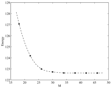
Figure 1: Convergence of the ground state energy as a function of the number of single-particle states $M$, for the case of $N=6$ electrons and a strong interaction $V_{C}=10$. The dashed line is to guide the eye.

• 

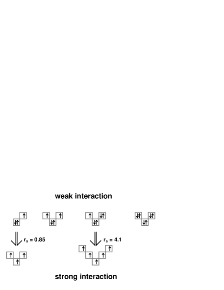
Figure 2: Single-particle states occupied in the VMC wave function. These are also the most important configurations in the ED expansion.

to closed-shell configuration at some point. For a three-electron ring, ED calculations show this transition to occur at an interaction strength of about $V_{C}\approx 0.41$, corresponding to $r_{s}\approx 0.85\,a_{B}^{*}$. For five electrons the transition takes place at $V_{C}\approx 3.3$ ($r_{s}\approx 4.1\,a_{B}^{*}$). The determinant part of the VMC wavefunction is chosen to be the relevant configuration shown in figure 2. These are the main configurations of the many-body state found by ED and have, at all except the strongest interaction, by far the largest weight in the determinant expansion.

• 

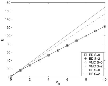
Figure 3: Total energy as a function of interaction strength for an $N=6$ electron ring of spin $S=0$ and $S=2$ and angular momentum $L=0$. Results from ED, VMC and HF are shown.

• 

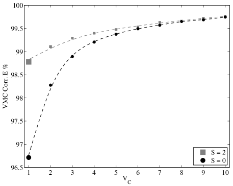
Figure 4: Percentage of correlation energy captured by VMC [see (30) for definition] for $N=6$ electrons, with $L=0$. The error in the the first two points is given by the marker size, and is smaller than that for the remaining points.

• 

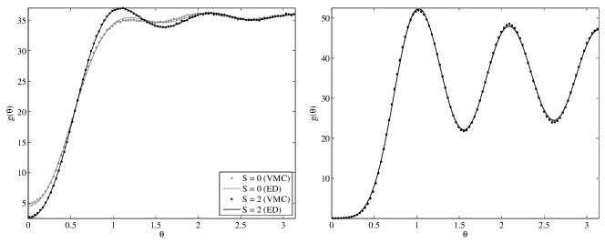
Figure 5: Pair distribution function from ED and VMC for $N=6$ electrons and $L=0$ with $S=0$ in gray and $S=2$ in black. On the left $V_{C}=1$ and on the right $V_{C}=10$. The dots show the VMC data while solid lines are the ED results. For strong interaction, the curves are nearly identical.

3.2 VMC accuracy

The total energy of six electrons on the ring is shown in figure 3. We have done the calculations for the $L=0$ state, and a total spin $S=0$ (groundstate) and $S=2$, and show the results obtained from ED, VMC and HF as a function of the strength of interaction (proportional to the ring radius). Over the whole range, ED and VMC results agree very well, although the agreement improves slightly with increasing $V_{C}$. The Hartree-Fock results are reasonably accurate only at the lowest interaction strength and already at $V_{C}=2$ (corresponding to $R=4\,a_{B}^{*}$ and $r_{s}=2.1\,a_{B}^{*}$) shows considerable deviation from the ED results.

To compare in more detail the results of ED and VMC, a convenient measure of the quality of the trial wave function is the percentage of correlation energy captured by VMC, defined as

$$E_{C}=\frac{E_{\rm HF}-E_{\rm VMC}}{E_{\rm HF}-E_{\rm ED}}\ ,$$ (30)

where $E_{\rm HF}$ is the Hartree-Fock energy. In figure 4 we show the results for the $L=0$ state of six electrons. At all interaction strengths, VMC captures most of the correlation energy. It is more accurate for the $S=2$ state than the $S=0$ state, although the difference decreases with increasing strength of interaction. One would expect VMC to become less accurate for strong interactions, because the construction of the VMC wave function starts from a single configuration which is later multiplied by a Jastrow factor, whereas the many-body wavefunction contains multiple determinants and their weights get more evenly distributed with increasing $V_{C}$. This is not the case, and at the highest $V_{C}$ the deviation in the VMC groundstate energy lacks such a single-configuration limitation. For other particle numbers the results are shown in table 1 for low and high interaction strength, $V_{C}=1$ and $V_{C}=10$. The VMC results are very accurate for the particle numbers we have considered. In the worst case, VMC captures 96% of the correlation energy and the total energy is roughly 0.7% higher than that found by ED. The accuracy improves with increasing interaction strength and is better for lower particle numbers. This trend is broken by cases where the major configuration has an open shell, which is always the case for odd particle numbers at weak interaction. This is demonstrated by five electrons, where VMC captures slightly less of the correlation energy than for six electrons.

Table 1: Percentages of correlation energy captured by VMC. The error in the last digit is given in parentheses.

• $V_{C}$	$N=4$	$N=5$	$N=6$
  1	0.9968(2)	0.9612(4)	0.9671(5)
  10	0.99909(5)	0.99917(6)	0.99746(7)

• 

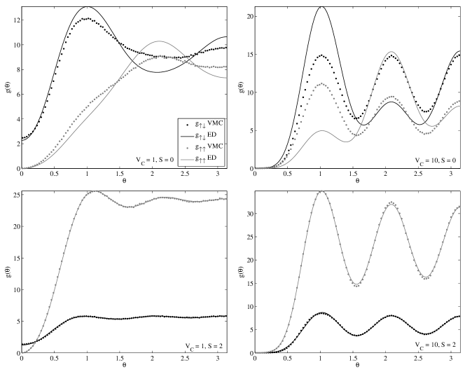
Figure 6: Spin channels in the pair distribution function from ED and VMC for $N=6$ electrons and $L=0$. The upper panel shows the results for the $S=0$ state and interaction strengths $V_{C}=1$ (left) and $V_{C}=10$ (right). The lower panel shows results for the $S=2$ state $V_{C}=1$ (left) and $V_{C}=10$ (right). The markers show the VMC data while solid lines are the ED results.

In figure 5, the total pair distribution function of an $N=6$ electron ring is shown at weak and strong interaction. As in the case of the groundstate energy, the agreement between VMC and ED is good. The left panel shows clearly how the total pair distribution functions of different spin states become identical when the electrons interact strongly. This is one indication of spin-charge separation, when the spin and charge of a one-dimensional system decouple.

The spin channels in the pair distribution function are shown in figure 6. For the $S=2$ state, VMC results are almost identical to those from ED. In the case of $S=0$, however, the internal structure is inaccurate at weak interaction and completely wrong at strong interaction. This is further shown in figure 7 where we have plotted

$$\Delta g=\frac{g_{\uparrow\uparrow}}{N_{\uparrow}-1}-\frac{g_{\uparrow\downarrow}}{N_{\downarrow}}\,,$$ (31)

which for an antiferromagnetic alignment of spins should give equidistant peaks (up spins) and troughs (down spins). This is indeed the case, and we furthermore see a decay in spin correlations with increasing interelectron distance. The VMC results show no antiferromagnetic structure. We believe the reason for VMC not being able to handle antiferromagnetic spin coupling is due to three-particle correlation which is missing in the VMC wavefunction. Despite VMC’s shortcomings in accurately describing the spin correlations for an antiferromagnetic spin structure, the total pair distribution function and the groundstate energy are correctly described.

• 

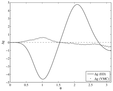
Figure 7: Pair distribution function difference, $\Delta g=g_{\uparrow\uparrow}/(N_{\uparrow}-1)-g_{\uparrow\downarrow}/N_{\downarrow}$, for six electrons in the state $L=0$, $S=0$. The ED results clearly indicate an antiferromagnetic structure.

3.3 Spin and charge in the Wigner crystal regime

Like the pair distribution function, the total energy of the $S=0$ and $S=2$ states becomes identical in the limit of strong interaction. In figure 8 we show the energy difference of these states for six electrons, as a function of $V_{C}$ found by ED, VMC and HF. The inset shows the energy difference found by ED on a logarithmic scale. As expected, HF fails seriously already at low values of $V_{C}$ and predicts a groundstate of nonzero spin-polarization at $V_{C}$ just below 1 ($r_{s}\approx 1$). VMC follows the ED results more closely, but at $V_{C}=4$ predicts a change in spin. ED results indicate, however, that the groundstate spin remains $S=0$ over the whole range of $V_{C}$ although the energy difference approaches zero. Interestingly, the difference between the ED and VMC results remains approximately constant for $V_{C}=4\dots 10$.

Figure 8 shows that in the strong interaction regime, the energy scale of spin dynamics becomes very small when compared to the energy scale of the orbital motion. This is one indication of a strong spin-charge separation in the system. It is further manifested in the pair distribution function, as shown in figure 5, which is the same for both spin states, $S=0$ and $S=2$, at stronger interaction. The spin part can be described by the antiferromagnetic Heisenberg model [13] with spin interaction

$$H_{\sigma}=J\sum_{i,j}{\bf S}_{i}\cdot{\bf S}_{j}$$ (32)

with a nearest-neighbour coupling constant $J$. In a recent paper, Fogler and Pivovarov [14] derived a relation between the coupling constant of thin quantum rings and the pair distribution function of a spin-polarized 1D system $g_{0}(x)$

$$J=\frac{\rme^{2}a_{B}^{2}}{2\ln(a_{B}/R^{*})\epsilon}\,g_{0}^{\prime\prime}(0)\,,$$ (33)

where $R^{*}$ is the thickness of the ring, in our case $\mu R$. For ultrathin wires exhibiting strong spin-charge separation, this relation holds even at moderate electron densities, $r_{s}\sim 1$. They furthermore derive an expression for the pair distribution function, which leads to

$$J=\frac{\kappa}{(2r_{s})^{5/4}}\frac{\pi}{\ln(a_{B}/R^{*})}\frac{\rme^{2}}{\epsilon a_{B}}\exp(-\eta\sqrt{2r_{s}})\ ,$$ (34)

where $\kappa$ and $\eta$ are constants.

• 

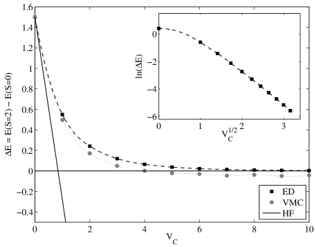
Figure 8: Difference in energy of the $S=0$ and $S=2$ states of six electrons with angular momentum $L=0$, as found by ED, VMC and HF. In the inset the logarithm of the energy difference is plotted against $\sqrt{V_{C}}$.

• 

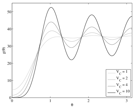
Figure 9: Pair distribution function of six electrons in the $L=0$, $S=0$ state for several values of the strength of interaction $V_{C}$.

• 

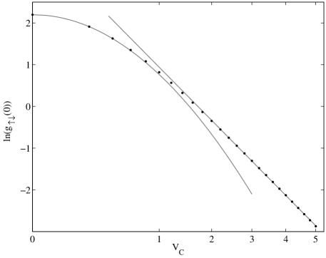
Figure 10: Logarithm of the contact probability $g_{\uparrow\downarrow}(0)$ of opposite spin electrons as a function of the strength of interaction $V_{C}$ on a square root scale. The parabolic curve is a guide to the eye only and indicates an exponential falloff with $V_{C}$. The straight line is a linear fit and indicates a $\exp(-\zeta\sqrt{V_{C}})$ behaviour.

The coupling constant $J$ is proportional to the difference in energy of the $S=0$ and $S=2$ states, $\Delta E$. In our model, $r_{s}=2\pi V_{C}/N$ so we can write

$$\Delta E\propto\exp(-\eta\sqrt{4\pi/N}\sqrt{V_{C}})\ .$$ (35)

In the inset of figure 8 we have plotted the logarithm of $\Delta E$ as a function of $\sqrt{V_{C}}$. Our results agree very well with the results of Fogler et al., as the curve becomes linear even at low values of $V_{C}$, $V_{C}\approx 1.7$ ($r_{s}\approx 1.8$). From our data we can estimate the slope, and find that $\eta\approx 2.5$ which is reasonably close to the value 2.7979 found by Fogler and Pivarov. However, it must be noted that our results are for a fixed value of $\mu=0.1$, so that the thickness of the ring scales linearly with increasing interaction strength as $R^{*}/a_{B}^{*}=0.1R=0.2\,V_{C}$.

The pair distribution function of six electrons of zero total angular momentum and spin is shown in figure 9 for several values of $V_{C}$. At $V_{C}=1$ the distribution is rather flat, but already at $V_{C}=2$ there is a clear peak structure indicating partial localization in relative coordinates. As the system is finite, a phase transition to a Wigner crystal does not take place. However, there is a smooth transition to a regime where a Wigner-crystal-like behaviour is found. The system is translationally invariant and the electron density remains uniform, the localization occurs in the relative frame. In two-dimensional quantum dots, the electrons are found to be localized at [25] $r_{s}=4$, and the transition is preceded by a change in the groundstate spin [26]. A QMC study of the three-dimensional electron gas showed an abrupt change in the evolution of the correlation energy with density [27]. We do not see such a change in our system. One should also note that the three-dimensional QMC work has different wave functions for the liquid and solid phase, whereas we use the same wave function in both cases.

Further insight is obtained from the value of the pair distribution function at $\theta=0$, which is the contact probability. At low values of the strength of interaction $V_{C}$ it has a nonzero value, as electrons of opposite spin are not restricted by the Pauli exclusion principle. As $V_{C}$ grows, the strong Coulomb repulsion reduces $g_{\uparrow\downarrow}(0)$ to the point where the electrons become localized between their neighbors on either side. A closer look at the contact probability reveals an indication that the quantum ring system undergoes a smooth transition at densities between $1<r_{s}<2$. In figure 10 the logarithm of the contact probability is shown as a function of the interaction strength on a square root scale. For $V_{C}\geq 2$, the linear fit indicates that $g_{\uparrow\downarrow}(0)$ falls off as $\exp(-\zeta\sqrt{V_{C}})$, where $\zeta$ is a constant. At low interaction strength, the behaviour is closer to $\exp(-\zeta^{\prime}V_{C})$, the parabolic curve shown. A related behaviour has been found for a different quantity in quantum dots [25].

4 Conclusions

We have studied interacting electrons in a one-dimensional quantum ring. We compared the results obtained from variational Monte Carlo with those of exact diagonalization. The variational wave function was taken to be of a simple Slater-Jastrow form: a single determinant, the ground state of the noninteracting system, multiplied by a two-body correlation factor. The results obtained indicate that this simple wave function is able to capture the important correlation effects, and in most cases even with a high accuracy.

The major source of error in VMC is the spin energy scale and spin correlation. The spin energy scale, however, becomes very small already at rather weak interaction and the error in the groundstate energy is correspondingly small and decreases with increasing $V_{C}$. For an antiferromagnetic spin correlation, VMC does not capture the internal spin structure, but the total pair distribution function is accurate. From this, one can conclude that the Jastrow factor is very efficient in capturing the total energy and essential correlation effects induced by the interaction between electrons. One might question the importance of the determinant part of the VMC wave function. We believe that having a good choice for this is crucial for the success of the VMC simulation. Even if the weight of this single configuration is not large in the exact expansion when the interaction is strong, it specifies the symmetry of the VMC many-body state. One should note that this is also the case for quantum dots, where the noninteracting single-particle states can be used in the determinant part of the VMC wave function, and they are even the optimal ones in the case of a closed-shell configuration [9]. The reason, both in quantum rings and dots, is the high symmetry of the problem: In a parabolic dot, the centre-of-mass and relative motion decouple, also in the many-body wave function. Thus if one starts from a noninteracting state that is a ground state of the centre-of-mass motion, the interactions only change the relative motion part of the many-body wave function. This means that if a Slater-Jastrow wave function is used, the Slater determinant part is not changed by the interaction between electrons. The case of a quantum ring is similar in the sense that the centre-of-mass and relative motion also decouple, but now because of the translational invariance of the system.

For a moderate strength of interaction, the spin correlation is well described by an antiferromagnetic Heisenberg model with coupling constant $J$. We showed that our results agree well with the expression for $J$ derived by Fogler and Pivovarov [14] at $r_{s}\gtrapprox 2$. Their result is applicable already at $r_{s}\sim 1$ if a strong spin-charge separation is present in the system. This indicates that for an ultrathin quantum ring this separation does take place at a quite high electron density. The contact probability also shows that there is a change in the properties of the system starting at $1<r_{s}<2$.

In conclusion, a simple variational wave function, combined with Monte Carlo techniques to calculate the optimal wave function and observables of the system, results in an efficient computational strategy for interacting electrons in purely one-dimensional quantum rings. Since a similar conclusion can be drawn for two-dimensional quantum dots [9], we expect this to hold also for quantum rings of a finite width.

References

- [1] Keyser U F, Fühner C, Borck S, Haug R J, Bichler M, Abstreiter G and Wegscheider W 2003 Phys. Rev. Lett. 90 196601
- [2] Kusmartsev F V 1991 J. Phys.: Condens. Matter 3 3199–3204
- [3] Jagla E A and Balseiro C A 1993 Phys. Rev. Lett. 70 639
- [4] Kusmartsev F V, Weisz J F, Kishore R and Takahashi M 1994 Phys. Rev. B 49 16234
- [5] Niemelä K, Pietiläinen P, Hyvönen P and Chakraborty T 1996 Europhys. Lett. 36 533
- [6] Deo P S, Koskinen P, Koskinen M and Manninen M 2003 Europhys. Lett 63 846
- [7] Emperador A, Pederiva F and Lipparini E 2003 Phys. Rev. B 68 115312
- [8] Hallberg K, Aligia A A, Kampf A P and Normand B 2004 Phys. Rev. Lett. 93 067203
- [9] Harju A 2005 J. Low. Temp. Phys. 140 181
- [10] Borrmann P and Harting J 2001 Phys. Rev. Lett. 86 3120
- [11] Räsänen E, Saarikoski H, Stavrou V N, Harju A, Puska M J and Nieminen R M 2003 Phys. Rev. B 67 235307
- [12] Harju A, Räsänen E, Saarikoski H, Puska M J, Nieminen R M and Niemelä K 2004 Phys. Rev. B 69 153101
- [13] Koskinen M, Manninen M, Mottelson B and Reimann S M 2001 Phys. Rev. B 63 205323
- [14] Fogler M M and Pivovarov E 2005 Phys. Rev. B 72 195344
- [15] Keyser U F 2002 Nanolithography with an atomic force microscope: quantum point contacts, quantum dots, and quantum rings Ph.D. thesis University of Hannover
- [16] Hylleraas E 1928 Z. Physik 48 469
- [17] Slater J C 1929 Phys. Rev. 34 1293
- [18] Condon E U 1930 Phys. Rev. 36 1121
- [19] Slater J C 1931 Phys. Rev. 38 1109
- [20] Löwdin P O 1955 Phys. Rev. 97 1474
- [21] Oitmaa J 2005 private discussion
- [22] Foulkes W M C, Mitas L, Needs R J and Rajagopal G 2001 Rev. Mod. Phys. 73 33
- [23] Laughlin R B 1987 in R E Prange and S M Girvin, eds, The Quantum Hall Effect (New York: Springer-Verlag) pp 233–301
- [24] Lin X, Zhang H and Rappe A M 2000 J. Chem. Phys. 112 2650–2654
- [25] Egger R, Häusler W, Mak C H and Grabert H 1999 Phys. Rev. Lett. 82 3320
- [26] Harju A, Siljamäki S and Nieminen R M 2002 Phys. Rev. B 65 075309
- [27] Drummond N D, Radnai Z, Trail J R, Towler M D and Needs R J 2004 Phys. Rev. B 69 085116