Delocalization transition of the selective interface model:
distribution of pseudo-critical temperatures

Abstract

According to recent progress in the finite size scaling theory of critical disordered systems, the nature of the phase transition is reflected in the distribution of pseudo-critical temperatures $T_{c}(i,L)$ over the ensemble of samples $(i)$ of size $L$. In this paper, we apply this analysis to the delocalization transition of an heteropolymeric chain at a selective fluid-fluid interface. The width $\Delta T_{c}(L)$ and the shift $[T_{c}(\infty)-T_{c}^{av}(L)]$ are found to decay with the same exponent $L^{-1/\nu_{R}}$, where $1/\nu_{R}\sim 0.26$. The distribution of pseudo-critical temperatures $T_{c}(i,L)$ is clearly asymmetric, and is well fitted by a generalized Gumbel distribution of parameter $m\sim 3$. We also consider the free energy distribution, which can also be fitted by a generalized Gumbel distribution with a temperature dependent parameter, of order $m\sim 0.7$ in the critical region. Finally, the disorder averaged number of contacts with the interface scales at $T_{c}$ like $L^{\rho}$ with $\rho\sim 0.26\sim 1/\nu_{R}$.

I Introduction

Heteropolymers containing both hydrophobic and hydrophilic components are of particular interest in biology review1 . In a polar solvent, these heteropolymers prefer conformations where the hydrophilic components are in contact with the polar solvent, whereas hydrophobic components avoid contacts with the solvent. The behavior of such heteropolymers in the presence of an interface separating two selective solvents, one favorable to the hydrophobic components and the other to the hydrophilic components, is less obvious, and has been much studied recently Fleer ; protein1 . In the initial work of ref. garel , a model was proposed and studied via Imry-Ma arguments, an analysis of the replica Hamiltonian and numerics : it was found that a chain with a symmetric distribution of hydrophobic/hydrophilic components is always localized around the interface at any temperature (in the thermodynamic limit), whereas a chain with a dissymmetric distribution of hydrophobic/hydrophilic components presents a phase transition separating a localized phase at low temperature from a delocalized phase into the most favorable solvent at high temperature. Experimentally, the presence of copolymers was found to stabilize the interface between the two immiscible solvents experiments , since the localization of the heteropolymers at the interface reduces the surface tension. By now, the predictions of ref. garel have been confirmed in the physics community by various approaches including molecular dynamics simulations yeung , Monte Carlo studies sommer ; Chen , variational methods for the replica Hamiltonian stepanow maritanreplica , exact bounds for the free-energy maritanbounds , and dynamical approach Gan_Bre . A real space renormalization group study, based on rare events, was proposed in CM2000 . Mathematicians have also been interested in this model. The localization at all temperatures for the symmetric case was proven in ref. sinai ; albeverio . In the dissymmetric case, the existence of a transition line in temperature vs dissymmetry plane was proven in ref. bolthausen ; biskup . Recently, important progresses were made in various aspects of the phase transition GT1 ; GT2 ; GT3 ; GT4 .

We study here the same model using the Wiseman-Domany approach to finite size scaling in disordered systems domany95 ; AH ; Paz1 ; domany ; AHW ; Paz2 . The main outcome of this approach can be summarized as follows. To each disordered sample $(i)$ of size $L$, one should first associate a pseudo-critical temperature $T_{c}(i,L)$, defined for instance in magnetic systems as the temperature where the susceptibility is maximum domany95 ; Paz1 ; domany ; Paz2 . The disorder averaged pseudo-critical temperature $T_{c}^{av}(L)\equiv\overline{T_{c}(i,L)}$ satisfies

$$T_{c}^{av}(L)-T_{c}(\infty)\sim L^{-1/\nu_{R}}$$ (1)

where $\nu_{R}$ is the correlation length exponent. Eq. (1) generalizes the analogous relation for pure systems

$$T_{c}^{pure}(L)-T_{c}(\infty)\sim L^{-1/\nu_{P}}$$ (2)

The nature of the disordered critical point then depends on the width

$$\Delta T_{c}(L)\equiv\sqrt{Var[T_{c}(i,L)]}=\sqrt{\overline{T_{c}^{2}(i,L)}-\left(\overline{T_{c}(i,L)}\right)^{2}}$$ (3)

of the distribution of pseudo-critical temperatures. When the disorder is irrelevant, the fluctuations of these pseudo-critical temperatures obey the scaling of a central limit theorem as in the Harris argument :

$$\Delta T_{c}(L)\sim L^{-d/2}\ \ \hbox{ for irrelevant disorder }$$ (4)

This behavior was first believed to hold in general domany95 ; Paz1 , but was later shown to be wrong in the case of random fixed points : in AH ; domany , it was argued that at a random critical point, one has instead

$$\Delta T_{c}(L)\sim L^{-1/\nu_{R}}\ \ \hbox{ for random critical points }$$ (5)

i.e. the scaling is the same as the $L$-dependent shift of the averaged pseudo-critical temperature (1). The fact that these two temperature scales remain the same is then an essential property of random fixed points that leads to the lack of self-averaging for observables at criticality AH ; domany .

In this paper, we apply this finite size scaling analysis to the case of the polymer chain at an interface between two selective fluids. The paper is organized as follows. The model is defined in Section II. The definition of pseudo-critical temperatures, and their distribution is presented in Section III. The distribution of the free energy difference between delocalized and localized phases is studied in Section IV. Finally, in Section V, we consider the averaged number of contacts with the interface. The numerical implementation through the Fixman-Freire procedure is postponed to the Appendix.

II Model and notations

II.1 Definition of the model

The model we consider is defined by the partition function

$$Z(L)=\sum_{\{z_{\alpha}\}}exp\left(\beta\sum_{\alpha}q_{\alpha}{\rm sgn}z_{\alpha}\right)$$ (6)

with inverse temperature $\beta=1/T$. The sum in (6) is over all random walks $\{z_{\alpha}\}$ of $L$ steps, with increments $z_{{\alpha}+1}-z_{\alpha}=\pm 1$ and (bound-bound) boundary conditions $z_{1}=0=z_{L}$. In eq. (6), the $\{q_{\alpha}\}$ represent quenched random charges, and with our convention, monomers with positive charges prefer to be in the upper fluid (${\rm sgn}z>0$). Furthermore, we have taken $q_{2{\alpha}+1}=0$ for all $(\alpha)$, so that there is no frustration at zero temperature (each monomer $z_{2{\alpha}}$ being in its preferred solvent). Even charges $q_{2{\alpha}}$ are random and drawn from the Gaussian distribution with mean value $q_{0}$ ($q_{0}>0$)

$$P(q_{2{\alpha}})=\frac{1}{\sqrt{2\pi\Delta^{2}}}e^{-\frac{(q_{2{\alpha}}-q_{0})^{2}}{2\Delta^{2}}}$$ (7)

From previous work, model (6) is expected to undergo a phase transition at a critical temperature $T_{c}\simeq O(\Delta^{2}/q_{0})$ between a localized phase and a delocalized phase in the upper fluid.

II.2 Recursion relations for the partition function

Let $Z(\alpha)$ be the partition function of the partial chain ($1,2,...\alpha$), with monomer ($\alpha$) sitting at the interface ($z_{\alpha}=0$). Since the last loop before monomer $(\alpha$) can be in the upper ($+$) or in the lower ($-$) fluid, we may write

$$Z(\alpha)=Z^{+}(\alpha)+Z^{-}(\alpha)$$ (8)

The partition functions $Z^{\pm}(\alpha)$ satisfy the recursions

$$Z^{\pm}(\alpha)=\sum_{\alpha^{\prime}=1,3,..}^{\alpha-2}exp\left(\pm\beta\sum_{i=\alpha^{\prime}+1}^{\alpha-1}q_{i}\right)\ {\cal N}(\alpha^{\prime},\alpha)\left[Z^{+}(\alpha^{\prime})+Z^{-}(\alpha^{\prime})\right]$$ (9)

where ${\cal N}(\alpha^{\prime},\alpha)$ represents the number of random walks of $(\alpha-\alpha^{\prime})$ steps going from $z_{\alpha^{\prime}}=0$ to $z_{\alpha}=0$, without touching the interface at $z=0$ in between. For the critical properties of the delocalization transition, the only important property of ${\cal N}(\alpha^{\prime},\alpha)$ is its behavior at large separation

$${\cal N}(\alpha^{\prime},\alpha)\mathop{\simeq}_{\alpha-\alpha^{\prime}\gg 1}\sigma\frac{2^{\alpha-\alpha^{\prime}}}{(\alpha-\alpha^{\prime})^{3/2}}$$ (10)

where $\sigma$ is a constant of order $1$. In our numerical study, we have chosen to take the following form

$${\cal N}(\alpha^{\prime},\alpha)=\sigma\frac{2^{\alpha-\alpha^{\prime}}}{(\alpha-\alpha^{\prime}-1)^{3/2}}$$ (11)

for all $(\alpha-\alpha^{\prime})$. If one forgets the boundary conditions at $(1,\alpha)$, the partition function characterizing the delocalized phase in the $(+)$ solvent ($q_{0}>0$) would simply be for each sequence of charges

$$Z^{deloc}(\alpha)=2^{\alpha-1}e^{\beta V(\alpha)}\ \ \ {\rm with}\ \ \ V(\alpha)\equiv\sum_{\alpha^{\prime}=2}^{\alpha}q_{i}$$ (12)

It is convenient to introduce the ratio

$${\tilde{Z}}(\alpha)\equiv\frac{Z(\alpha)}{Z^{deloc}(\alpha)}={\tilde{Z}}^{+}(\alpha)+{\tilde{Z}}^{-}(\alpha)$$ (13)

where ${\tilde{Z}}^{\pm}(\alpha)\equiv Z^{\pm}(\alpha)/Z^{deloc}(\alpha)$ satisfy the recursion relations (Eq. 9)

$${\tilde{Z}}^{+}(\alpha) =\sum_{\alpha^{\prime}=1,3,..}^{\alpha-2}\frac{\sigma}{(\alpha-\alpha^{\prime}-1)^{3/2}}\left[{\tilde{Z}}^{+}(\alpha^{\prime})+{\tilde{Z}}^{-}(\alpha^{\prime})\right]$$

$${\tilde{Z}}^{-}(\alpha) =\sum_{\alpha^{\prime}=1,3,..}^{\alpha-2}e^{-2\beta\left(V(\alpha-1)-V(\alpha^{\prime})\right)}\frac{\sigma}{(\alpha-\alpha^{\prime}-1)^{3/2}}\left[{\tilde{Z}}^{+}(\alpha^{\prime})+{\tilde{Z}}^{-}(\alpha^{\prime})\right]$$ (14)

The numerical iteration of Eqs (14) takes a CPU time of order $O(L^{2})$ for a chain of length $L$, but it is possible to obtain a CPU time of order $O(L)$ via a Fixman-Freire scheme Fix_Fre . Originally proposed in the context of the Poland-Scheraga model of DNA denaturation, this scheme can be adapted to the interface model, as explained in the Appendix.

II.3 Numerical parameters

We have taken $q_{0}=1$ and $\Delta=10$ in the Gaussian distibution of eq (7). The data we present correspond to various sizes $L$ with corresponding numbers $n_{s}(L)$ of independent samples. Unless otherwise stated, we have considered the following sizes going from $L=2\cdot 10^{3}$ to $L=2048\cdot 10^{3}$, with respectively $n_{s}(L=16\cdot 10^{3})=480\cdot 10^{3}$ to $n_{s}(L=2048\cdot 10^{3})=15\cdot 10^{3}$. More precisely, we consider

$$\frac{L}{1000} =16,32,64,128,256,512,1024,2048$$ (15)

$$\frac{n_{s}(L)}{1000} =480,240,120,60,30,15,30,15$$ (16)

III Distribution of Pseudo critical temperatures

In a previous paper PSdisorder , we have discussed two possible definitions for the pseudo-critical temperatures for Poland-Scheraga models. Here we use the definition based on the free energy, as we now explain.

III.1 Definition of a sample dependent $T_{c}(i,L)$

For each sample $(i)$ of length $L$, we may define a pseudo-critical temperature $T_{c}(i,L)$ as the temperature where the free energy $F^{(i)}(L,T)\equiv-T\ln Z^{(i)}(L,T)$ reaches the delocalized value $F_{deloc}^{(i)}(L,T)=-T(L-1)\ln 2-V(L)$ (Eq. 12), i.e. $T_{c}(i,L)$ is the solution of the equation

$$F^{(i)}(L,T)+T(L-1)\ln 2+V(L)=0$$ (17)

As explained in details in our previous study PSdisorder , this definition of pseudo-critical critical temperatures, together with bound-bound boundary conditions, introduces logarithmic correction in the convergence towards $T_{c}(\infty)$. Eq. (1) is accordingly replaced by

$$T_{c}^{av}(L)-T_{c}(\infty)\sim\left(\frac{\ln L}{L}\right)^{1/\nu_{R}}$$ (18)

III.2 Scaling form of the probability distribution

Our data for the distribution of pseudo-critical temperatures (see Figure 1) follow the scaling form

$$P_{L}(T_{c}(i,L))\simeq\frac{1}{\Delta T_{c}(L)}\ g\left(x=\frac{T_{c}(i,L)-T_{c}^{av}(L)}{\Delta T_{c}(L)}\right)$$ (19)

where the scaling distribution $g(x)$ (normalized with $<x>=0$ and $<x^{2}>=1$) is well fitted by the one parameter generalized Gumbel distribution $G_{m}(-x)$

$$g(x)=G_{m}(-x)\equiv\frac{m^{m}}{\Gamma(m)}\left(e^{-x-e^{-x}}\right)^{m}$$ (20)

with parameter $m\sim 3$. On Fig. 1(b), we show the fit of our data with $G_{3}(-x)$, and plot for comparison the usual Gumbel ($m=1$) and Gaussian ($m\to\infty$) distributions.

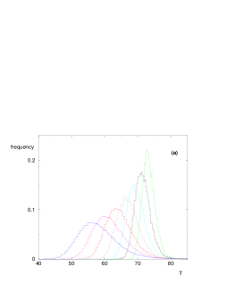
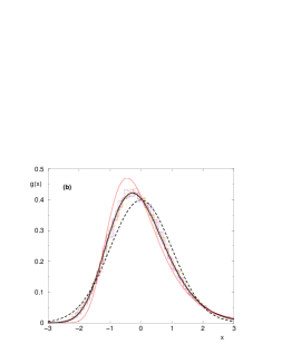
Figure 1: (a) Distribution of critical temperatures for ($L/10^{3}=32,64,128,256,512,1024,2048$) (b) Same data after the rescaling of eq. (19): fit with the generalized Gumbel distribution $G_{3}(-x)$ (thick line). For comparison, we also show the usual Gumbel $m=1$ (thin line) and Gaussian $m=\infty$ (dashed line) distributions.

III.3 Scaling properties of the shift and of the width

We now consider the behavior of the width $\Delta T_{c}(L)$ and of the average $T_{c}^{av}(L)$ of the distribution (19), as $L$ varies. For the width $\Delta T_{c}(L)$, we have fitted our data with the following power law (see Fig 2(a))

$$\Delta T_{c}(L)\simeq 86\left(\frac{1}{L}\right)^{0.26}$$ (21)

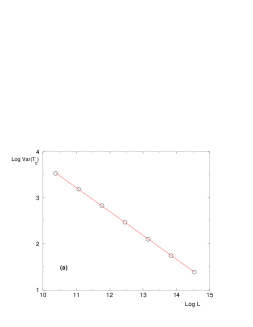
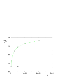
Figure 2: (a) Log-Log plot of the variance ${Var[T_{c}(i,L)]}=(\Delta T_{c}(L))^{2}$ for $L/10^{3}=32,64,128,256,512,1024,2048$ ($\bigcirc$) with the fit of equation (21) (b) The average $T_{c}^{av}(L)$ for the same sizes, with the fit of equation (22) .

For the average $T_{c}^{av}(L)$ (see Fig 2(b)), our data are well fitted by the generalized form of eq. (18)

$$T_{c}^{av}(L)\simeq 83.8-246\left(\frac{\ln(L/289)}{L}\right)^{0.26}$$ (22)

The value $T_{c}(\infty)\simeq 83.8=0.838\frac{\Delta^{2}}{q_{0}}$ is in agreement with the numerical estimate of ref GT3 . The result for the exponent in eqs (21) and (22) indicate that the transition can be described as a random critical point with a single correlation exponent

$$\frac{1}{\nu_{R}}\simeq 0.26$$ (23)

A similar value has been observed in numerical simulations by the authors of ref. GT3 (private commnunication ).

Our data rule out the possibility of an infinite order transition based on rare negatively charged sequences CM2000 . The present results suggest that the excursions in the unfavorable fluid that are important for the transition, are of finite length.

IV Free energy distribution

Since the distribution of pseudo critical temperature is clearly linked to the statistical properties of the free energy, we have studied the probability distribution of the free energy difference $\tilde{F}^{(i)}(L,T)$ defined by (see eq. 17)

$$\tilde{F}^{(i)}(L,T)\equiv F^{(i)}(L,T)-F_{deloc}^{(i)}(L,T)=F^{(i)}(L,T)+T(L-1)\ln 2+V(L)$$ (24)

Defining the average $\tilde{F}^{(av)}(L,T)$ and the width $\Delta\tilde{F}(L,T)$, we write the scaled probability distribution as

$$P(\tilde{F}^{(i)}(L,T))\simeq\frac{1}{\Delta\tilde{F}(L,T)}\ h_{T}\left(x=\frac{\tilde{F}^{(i)}(L,T)-\tilde{F}^{(av)}(L,T)}{\Delta\tilde{F}(L,T)}\right)$$ (25)

where the function $h_{T}(x)$ is independent of $L$, but depends on the temperature $T$. We show in Figure 3 the function $h_{T}(x)$ for $T=40$ (deep in the localized phase), $T=82$ (critical region) and $T=130$ (deep in the delocalized phase).

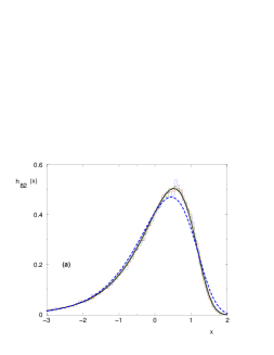
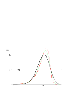
Figure 3: (a) Fit of the rescaled free energy distribution $h_{T}(x)$ (eq.(25)) at $T=82$ for $L/10^{3}=32,64,128,256,512$ by the generalized Gumbel distribution $G_{m}(x)$ with $m=0.66$ (thick line). The usual Gumbel distribution ($m=1$) is also shown for comparison (dashed line) (b) The function $h_{T}(x)$ for $L/10^{3}=32$ at $T=40$ (thick solid line), $T=82\sim T_{c}$ (dashed line) and $T=130$ (thin solid line). Fitting with the generalized Gumbel distribution $G_{m}(x)$ leads to a non monotonous variation of $m$ w.r.t the temperature $T$. The minimal value of $m$ is obtained in the critical region.

It turns out that a good one parameter fit is again obtained with the generalized Gumbel distribution

$$h_{T}(x)=G_{m}(x)\equiv\frac{m^{m}}{\Gamma(m)}\left(e^{x-e^{x}}\right)^{m}$$ (26)

where the effective parameter $m$ depends on the temperature $T$. We now characterize the behaviour at low and high temperatures, as well as in the critical region.

IV.1 The localized phase

At $T\ll T_{c}$, the sample dependent free energy $\tilde{F}^{(i)}(L,T)$ can be fitted by

$$\tilde{F}_{i}(L,T)=Lf_{\infty}(T)+\sigma_{T}\sqrt{L}\ u_{i}+O(1)$$ (27)

where $u_{i}$ is a Gaussian random variable (which corresponds to the Gumbel parameter $m\to\infty$). Eq. (27) is indeed expected from the existence of an extensive number of contacts with the interface: fluctuations are then of order $\sqrt{L}$ and Gaussian distributed.

IV.2 The delocalized phase

At $T\gg T_{c}$ the sample dependent free energy $\tilde{F}_{i}(L,T)$ can be fitted by

$$\tilde{F}_{i}(L,T)=\frac{3}{2}T\ {\rm Ln}\frac{L}{l_{0}}+v_{i}$$ (28)

where $l_{0}$ is a constant, and $v_{i}$ is a random variable distributed with $G_{m}(x)$ and $m\sim 1.3$ (see eq. (26). The first term on the r.h.s of eq.(28) comes from the bound-bound boundary conditions, while the random term of order $O(1)$ reflects rare contacts with the interface.

IV.3 In the critical region

In the critical region, the average free energy $\tilde{F}^{(av)}(L,T)$ behaves as

$$\tilde{F}^{(av)}(L,T)=Lf_{\infty}(T)+f_{1}(T)\ {\rm Ln}\frac{L}{l_{0}}$$ (29)

where $f_{1}$ is a coefficient which weakly depends on temperature in the critical region. The thermodynamic free energy density $f_{\infty}(T)$ is then found to go to zero between $T=82$ and $T=83$, in good agreement with the value $T_{c}\simeq 83.8$ obtained above. Concerning the rescaled distribution $h_{T}(x)$, we observe that the parameter $m$ remains at a minimum value of order $0.7$ in a large temperature range $75<T<85$. This large crossover region is clearly linked to the small value of $1/\nu_{R}\sim 0.26$.

V Contacts

We have also considered the disorder averaged number of contacts $N_{0}$ with the interface in the critical region, and we numerically obtain

$$N_{0}(T_{c},L)=\sum_{\alpha=1}^{L}\overline{<\delta(z_{\alpha},0)>_{T_{c}}}\sim L^{\rho}\ ,\ \rho\sim 0.26$$ (30)

It is interesting to compare this result with the behavior of the internal energy difference $E_{0}(T,L)$ between the localized and delocalized phases. A simple scaling argument based on the hyperscaling relation $\alpha=2-\nu_{R}$ yields the following behavior for the energy $E_{0}(T_{c},L)\sim L^{1/\nu_{R}}$ at criticality. The fact that the exponent $\rho$ is close to the exponent $1/\nu_{R}$ points towards the same scaling for the energy and number of excursions in the unfavorable fluid : this means that, at criticality, the excursions in the lower unfavorable fluid are of finite length.

Finally, our data on the number of contacts $N_{0}(T,L)$ yield an estimate of the critical temperature $82.5<T_{c}<83$, which is again compatible with the above mentionned values.

VI Conclusion

We have studied the probability distribution finctions (PDF) of the pseudo-critical temperatures $T_{c}(i,L)$ and of the free energy $\tilde{F}_{i}(L,T)$ for the localization transition of an heteropolymer at a selective fluid-fluid interface. We have obtained an estimate of the critical temperature $T_{c}\sim 0.83\frac{\Delta^{2}}{q_{0}}$, in agreement with GT3 . Both the width $\Delta T_{c}(L)$ and the shift $[T_{c}(\infty)-T_{c}^{av}(L)]$ are found to decay with the same exponent $L^{-1/\nu_{R}}$ where $1/\nu_{R}\sim 0.26$. These results show that the transition is not due to rare events, such as large excursions in the unfavorable fluid CM2000 .

Concerning the form of the PDF’s, we find here asymmetric distributions, which can fitted with generalized Gumbel distributions $G_{m}(x)$. This is in contrast with the wetting and Poland-Scheraga transitions PSdisorder , where these PDF’s were found to be Gaussian. Generalized Gumbel distributions have been recently used in various contexts Bramwell ; BBW ; Palassini ; Rosso ; Bertin . As discussed in ref. Bramwell , it is empirically known that PDF’s with the same first four moments approximately coincide over the range of a few standard deviation which is precisely the range of numerical -or experimental- data. So generalized Gumbel PDF’s, with arbitrary $m$, should probably not be considered more than a a convenient one parameter fit (for instance, Tracy-Widom distributions defined in terms of Airy functions prae , can be also fitted very well by generalized Gumbel distributions in the range of interest).

Appendix A Fixman-Freire scheme for the interface model

The Fixman-Freire scheme Fix_Fre , invented in the context of DNA denaturation, allows one to compute melting curves of DNA sequences in a CPU time of order $O(L)$ instead of $O(L^{2})$. Here we briefly explain how to adapt the Fixman-Freire method to the interface model.

The first step consists in replacing the factor $1/(\alpha-\alpha^{\prime}-1)^{3/2}$ appearing in the recursion relations (Eq. 14) by

$$\frac{1}{(\alpha-\alpha^{\prime}-1)^{3/2}}\simeq\sum_{i=1}^{I}a_{i}\ e^{-b_{i}(\alpha-\alpha^{\prime}-1)}$$ (31)

where the number ${I}$ of couples $(a_{i},b_{i})$ depends on the desired accuracy. The parameters $(a_{i},b_{i})$ are determined by a set of non-linear equations. This procedure has been tested on DNA chains of length up to $L=10^{6}$ base pairs Meltsim ; Yer , and the choice ${I}=15$ gives an accuracy better than $0.3\%$ and we have adopted this value. The table of parameters $(a_{i},b_{i})$ we have used can be found in our previous work on the wetting transition wetting2005 .

Let us now introduce the following notations

$$R^{\pm}(\alpha) \equiv\frac{{\tilde{Z}}^{\pm}(\alpha)}{{\tilde{Z}}(\alpha)}$$ (32)

$$\frac{1}{S(\alpha)} \equiv\frac{{\tilde{Z}}(\alpha)}{{\tilde{Z}}(\alpha)}=R^{+}(\alpha)+R^{-}(\alpha)$$ (33)

as well as the coefficients $\mu_{j}^{\pm}(\alpha)$ defined in terms of the Fixman-Freire coefficients $(b_{j})$ (Eq. 31) where $j=1,2,...I=15$

$$\mu^{+}_{j}(\alpha-2) =e^{-b_{j}(\alpha-4)}\sum_{\alpha^{\prime}=1,3,..}^{\alpha-4}e^{b_{j}\alpha^{\prime}}S(\alpha-2)S(\alpha-4)...S(\alpha^{\prime}+2)$$ (34)

$$\mu_{j}^{-}(\alpha-2) =e^{-b_{j}(\alpha-4)-2\beta V(\alpha-4)}\sum_{\alpha^{\prime}=1,3,..}^{\alpha-4}e^{b_{j}\alpha^{\prime}+2\beta V(\alpha^{\prime})}S(\alpha-2)S(\alpha-4)...S(\alpha^{\prime}+2)$$ (35)

It is then easy to obtain that for any $j$, these coefficients satisfy the simple recursions

$$\mu^{+}_{j}(\alpha) =S(\alpha)\left[1+e^{-2b_{j}}\mu^{+}_{j}(\alpha-2)\right]$$ (36)

$$\mu_{j}^{-}(\alpha) =S(\alpha)\left[1+e^{-2b_{j}-2\beta q_{\alpha-3}}\mu^{-}_{j}(\alpha-2)\right]$$ (37)

In terms of these coefficients, the recursions (Eq. 14) become for the ratios $R^{\pm}(\alpha)$ (Eq. 33)

$$R^{+}(\alpha) =\sigma\left[1+\sum_{j=1}^{I}a_{j}e^{-3b_{j}}\mu^{+}_{j}(\alpha-2)\right]$$

$$R^{-}(\alpha) =\sigma e^{-2\beta q_{\alpha-1}}\left[1+e^{-2\beta q_{\alpha-3}}\sum_{j=1}^{I}a_{j}e^{-3b_{j}}\mu^{-}_{j}(\alpha-2)\right]$$ (38)

The recursions (37,38) can now be iterated in a CPU time of order $O(L)$.

References

- (1) T. Garel, H. Orland and E. Pitard, “Protein folding and heteropolymers”, in Spin Glasses and Random Fields, A.P. Young (ed.), World Scientific, Singapore (1997) p. 387-443.
- (2) G.J. Fleer, M.A. Cohen-Stuart, J.M.H.M. Scheutjens, T. Cosgrove and B. Vincent, Polymers at interfaces, Chapman and Hall (1994).
- (3) Proteins at liquid interfaces, D. Möbius and R. Miller Eds, Studies in Interface Science vol. 7, Elsevier (1998).
- (4) T. Garel, D.A. Huse, L. Leibler and H. Orland, Europhys. Lett. 8, 9 (1989).
- (5) H.R. Brown, V.R. Deline and P.F. Green, Nature 341 , 221 (1989); C.A. Dai, B.J. Dair, K.H. Dai, C.K. Ober, E.J. Kramer, C.Y. Hui and L.W. Jelinsky, Phys. Rev. Lett. 73 , 2472 (1994).
- (6) C. Yeung, A.C. Balazs and D. Jasnow, Macromolecules, 25 , 1357 (1992).
- (7) J.U. Sommer, G. Peng and A. Blumen, Phys. Rev. E 53 5509 (1996); J. Phys. II France 6 1061 (1996); J. Chem. Phys. 105 8376 (1996).
- (8) S. Stepanow, J.U. Sommer, and I.Y. Erukhimovich, Phys. Rev. Lett. 81 4412 (1998).
- (9) A. Trovato and A. Maritan, Europhys. Lett. 46, 301 (1999)
- (10) A. Maritan, M.P. Riva and A. Trovato, J.Phys. A, 32, L275 (1999).
- (11) V. Ganesan and H. Brenner, Europhys. Lett., 46, 43 (1999).
- (12) Z. Y. Chen, J. Chem. Phys., 111, 5603 (1999); ibid., 112, 8665 (2000); ibid. 113, 10377 (2000).
- (13) C. Monthus, Eur.Phys. J, 13, 111 (2000).
- (14) Y.G. Sinai, Theor. Prob. Appl. 38 , 382 (1993).
- (15) S. Albeverio and X.Y. Zhou, J. Stat. Phys. 53 , 573 (1996).
- (16) E. Bolthausen and F. den Hollander, Ann. Prob. 25 , 1334 (1997).
- (17) M. Biskup and F. den Hollander, Ann. Appl. Prob., 9, 668 (1999).
- (18) T. Bodineau and G. Giacomin, J. Stat. Phys. 117, 801 (2004).
- (19) G. Giacomin and F.L. Toninelli, math.PR/0502394, Probab. Theor. Rel. Fields (Online, 2005).
- (20) F. Caravenna, G. Giacomin and M. Gubinelli, preprint, to appear in J. Stat. Phys.
- (21) G. Giacomin and F.L. Toninelli, math.PR/0510047
- (22) S. Wiseman and E. Domany, Phys Rev E 52, 3469 (1995).
- (23) A. Aharony, A.B. Harris, Phys Rev Lett 77, 3700 (1996).
- (24) F. Pázmándi, R.T. Scalettar and G.T. Zimányi, Phys. Rev. Lett. 79, 5130 (1997).
- (25) S. Wiseman and E. Domany, Phys. Rev. Lett. 81, 22 (1998) ; Phys Rev E 58, 2938 (1998).
- (26) A. Aharony, A.B. Harris and S. Wiseman, Phys. Rev. Lett. 81, 252 (1998).
- (27) K. Bernardet, F. Pázmándi and G.G. Batrouni, Phys. Rev. Lett. 80, 4477 (2000).
- (28) M. Fixman and J.J. Freire, Biopolymers, 16, 2693 (1977)
- (29) C. Monthus and T. Garel, cond-mat/0509479.
- (30) T. Garel and C. Monthus, Eur. Phys. J. B, 46, 117 (2005).
- (31) S.T. Bramwell et al., Phys. Rev. Lett., 84, 3744 (2000); Phys. Rev. E, 63, 041106 (2001).
- (32) B.A. Berg, A. Billoire and W. Janke, Phys. Rev. E, 65, 045102 (2002).
- (33) M. Palassini, cond-mat/0307713 and references therein.
- (34) C.J. Bolech and A. Rosso, Phys. Rev. Lett., 93, 125701 (2004).
- (35) E. Bertin, Phys. Rev. Lett., 95, 170601 (2005) and references therein.
- (36) M. Prähoher and H. Spohn, http://www-m5.ma.tum.de/KPZ/.
- (37) R.D. Blake, J.W. Bizarro, J.D. Blake, G.R. Day, S.G. Delcourt, J. Knowles, K.A. Marx and J. SantaLucia Jr., Bioinformatics, 15, 370-375 (1999); see also J. Santalucia Jr., Proc. Natl. Acad. Sci. USA, 95, 1460 (1998).
- (38) E. Yeramian, Genes, 255, 139, 151 (2000).