Impact of boundaries on velocity profiles in bubble rafts

Abstract

Under conditions of sufficiently slow flow, foams, colloids, granular matter, and various pastes have been observed to exhibit shear localization, i.e. regions of flow coexisting with regions of solid-like behavior. The details of such shear localization can vary depending on the system being studied. A number of the systems of interest are confined so as to be quasi-two dimensional, and an important issue in these systems is the role of the confining boundaries. For foams, three basic systems have been studied with very different boundary conditions: Hele-Shaw cells (bubbles confined between two solid plates); bubble rafts (a single layer of bubbles freely floating on a surface of water); and confined bubble rafts (bubbles confined between the surface of water below and a glass plate on top). Often, it is assumed that the impact of the boundaries is not significant in the “quasi-static limit”, i.e. when externally imposed rates of strain are sufficiently smaller than internal kinematic relaxation times. In this paper, we directly test this assumption for rates of strain ranging from $10^{-3}$ to $10^{-2}\ {\rm s^{-1}}$. This corresponds to the quoted rate of strain that had been used in a number of previous experiments. It is found that the top plate dramatically alters both the velocity profile and the distribution of nonlinear rearrangements, even at these slow rates of strain. When a top is present, the flow is localized to a narrow band near the wall, and without a top, there is flow throughout the system.

I Introduction

When systems are driven sufficiently far from equilibrium, they often exhibit a series of transitions due to instabilities. This is particularly common in the flow of fluids, where instabilities occur at high flow rates. In contrast to this behavior, for sufficiently slow driving, complex fluids have been observed to undergo a transition from a purely flowing state to a coexistence between a flowing and a solid-like state, i.e. shear localization Howell et al. (1999); Mueth et al. (2000); Losert et al. (2000); Debrégeas et al. (2001); Coussot et al. (2002); Lauridsen et al. (2004); Huang et al. (2005); Salmon et al. (2003a, b). In this context, we focus on complex fluids that are comprised of dense “droplets” (or particles) of one phase or material within a different continuous phase, such as foams, emulsions, granular matter, and colloids. We are interested in the case where the droplets are sufficiently dense that there exists a critical value of applied stress, the yield stress, below which the material does not flow at all. In this situation, it has been observed that under conditions of non-uniform stress the material segregates into a region that flows (above the yield stress) and a region that does not flow (below the yield stress) BOO . However, because most of these materials are optically opaque, it is only recently that the spatial dependence of the average velocity of the “droplets” in these materials has been measured quantitatively. For three dimensional systems, a key development for such studies has been the development of magnetic-resonance-imaging Coussot et al. (2002) techniques that allow for spatially resolved velocity profiles. Equally useful has been the use of quasi-two dimensional systems in which all the droplets can be imaged Debrégeas et al. (2001); Lauridsen et al. (2004). Coupled with the experimental advances, there have been a number of simulations that explicitly look at the possibility of shear localization within the context of various models of granular matter and foams Varnik et al. (2003); Kabla and Debrégeas (2003); Xu et al. (2005a, b).

A striking feature of the experimental studies of shear localization in complex fluids is the division of the velocity profiles into two basic categories. The first situation corresponds to cases where the rate of strain is continuous across the system Howell et al. (1999); Mueth et al. (2000); Losert et al. (2000); Debrégeas et al. (2001). In this case, the spatial dependence of the velocity is often exponential. This appears to be the standard case for granular systems Howell et al. (1999); Mueth et al. (2000); Losert et al. (2000) and bubbles confined between two plates Debrégeas et al. (2001). In contrast, a discontinuity in the rate of strain at the transition between the flowing state and the jammed state is observed in emulsions and colloids Coussot et al. (2002), wet granular systems Huang et al. (2005), worm-like micelles Salmon et al. (2003a, b), three dimensional foams Rodts et al. (2005), and bubble rafts Lauridsen et al. (2004).

In comparing the systems mentioned above, it is useful to note that the systems were all sheared between two concentric cylinders. In this geometry, there is a non-uniform stress across the system. This might suggest that the localization is due to the “simple” picture that part of the system is above the yield stress and part of the system is below the yield stress. Surprisingly, there are a number of ways in which the experiments suggest that this explanation is not sufficient. For example, some of the systems (especially dry granular systems Losert et al. (2000)) clearly exhibit density variations that impact the flow behavior. An understanding of these variations is necessary for understanding the flow localization in these cases. In other studies, such as with wet granular matter, there are strong indications that the shear localization is the result of a viscosity bifurcation Huang et al. (2005).

In contrast to the experiments, simulations have focused on parallel shear. In this case, a linear velocity transverse to the shear is expected, and a nonlinear velocity profile is an indication of some type of shear localization. As with the experiments, simulations exhibit different behaviors depending on the details of the model. For example, shear localization is observed below a critical rate of strain Varnik et al. (2003); Kabla and Debrégeas (2003) and under different conditions, above a critical rate of strain Xu et al. (2005a).

For foam the situation is particularly interesting. For three-dimensional foam, both localized flow Rodts et al. (2005) and flow throughout the system Gopal and Durian (1999); Rouyer et al. (2003) have been observed. For quasi-two dimensional experiments, dramatically different types of flow localization has been observed depending on whether or not the bubbles were confined between two plates Debrégeas et al. (2001) or a bubble raft was used Lauridsen et al. (2004). These last two experiments highlight the need for a systematic study of the impact of the confining plates when studying quasi-two dimensional systems. In these systems, there is always a lower boundary supporting and confining the system, and depending on the experiment, there is often an upper boundary. Typically, the external shear is generated by motion of the sides, with the upper and lower boundaries held fixed. Because the focus is understanding the behavior under conditions of small applied rates of strain, the systems are often described as being in a quasi-static limit. If true, the expectation is that the interaction with the confining boundaries is irrelevant. However, the previous experiments Debrégeas et al. (2001); Lauridsen et al. (2004) indicate that the boundaries play a critical role, and suggest that one is not truly in a quasi-static regime, even though the behavior is rate independent QUA .

The flow behavior reported on in Refs. Debrégeas et al. (2001); Lauridsen et al. (2004) used a Couette geometry, i.e. flow between concentric cylinders. For bubbles confined between two plates, the shear localization corresponds to an exponentially decaying velocity as a function of the distance from the inner cylinder Debrégeas et al. (2001). For the case of a bubble raft (a single layer of bubbles floating on the surface of water Bragg and Lomer (1949); Argon and Kuo (1979); Mazuyer et al. (1989)), the velocity as a function of distance from the inner cylinder exhibited a discontinuity in the rate of strain Lauridsen et al. (2004). For the case of the confined bubbles, simulations suggest that nonlinear rearrangements of bubbles (known as T1 events) provided a focusing of the stress field that produced the shear localization Kabla and Debrégeas (2003). A T1 event corresponds to a neighbor switching where two neighboring bubbles separate, and two bubbles that were not neighbors become neighbors (see Fig. 1). For the bubble raft, the distribution of T1 events were studied and no localization was observed Dennin (2004).

As discussed, the most striking difference between the two experiments is the boundary conditions on the “top” and “bottom” of the bubbles. The experiments in the confined geometry have a glass plate in contact with the bubbles both on the top and the bottom. For the bubble raft, the top surface is free, as the bubble float on a water surface. There is a third geometry that has commonly been used to study quasi-two dimensional foam: a bubble raft with a top plate in contact with the bubbles. For example, this has been used to study quasi-static strains Kader and Earnshaw (1999) and the flow around obstacles Dollet et al. (2005). In this paper, we report on experimental studies aimed at determining the impact of the various boundary conditions. For the purposes of this comparison, we have focused on relatively monodisperse systems subjected to parallel shear. Monodisperse bubbles were used because these systems were the most reproducible between the two geometries. To allow for minimal variation between the systems while varying the boundary conditions, we focused on the two bubble raft systems: with and without a top. For comparison with past experiments, we consider a range of rate of strain that was consistent with the rates of strain used in Ref. Kabla and Debrégeas (2003); Lauridsen et al. (2004).

The remainder of the paper is organized as follows. Section II describes the apparatus and methods for producing the bubble rafts in detail. Section III describes the method for analyzing the bubble dynamics, especially the identification of T1 events. Finally, Sec. IV presents the results and the discussion of the results.

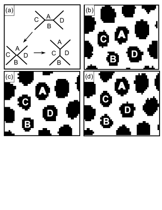
Figure 1: (a) Schematic representation of a T1 event illustrating two neighboring bubbles (A and B) switching to next nearest neighbor, and two next nearest neighbors (C and D) becoming neighbors. (b),(c),(d) A sequence of images that have been thresholded to bubbles are black taken from a bubble raft illustrating illustrating a T1 event.

II Experimental Details

The experimental setup contains three parts: the trough, the driving system and the imaging system. A schematic of the trough is given in Fig. 2. The trough consists of a rectangular Delarin dish (indicated by (A) in the Fig. 2) that is $300\ {\rm mm}\times 400\ {\rm mm}\times 75\ {\rm mm}$. This serves as the main reservoir for the aqueous solution. Inside this dish is a Teflon frame (indicated by (B)) that is used to establish a symmetric boundary and can support a glass top (not shown in Fig. 2). The frame is held by four poles and controlled by four micrometers outside of the trough (not shown). The size of the frame is $180\ {\rm mm}\times 300\ {\rm mm}\times 10\ {\rm mm}$. The frame can move in three dimensions, with adjustments in the plane used to maintain symmetric lateral boundaries. The vertical adjustment of the frame controls the height of the glass top relative to the bubbles.

The bubbles are driven by two counter-rotating belts (indicated by (C) in Fig. 2) using a stepper motor. As indicated in Fig. 2, we define the direction parallel to the belts to be the x-direction and the direction perpendicular to the belts as the y-direction. The stepper motor is a Mdrive 23 motor from Intelligent Motion System, Inc, model number MDMF2222, with microstepping capability. For driving the foam, the motor is set to 51200 microstep/rotation. The shafts, gears and belts are from W.M. Berg Inc. The driving bands are $210\ {\rm mm}$ long and spaced $57\ {\rm mm}$ apart. All the shafts are mounted at the bottom of the trough. The shafts are arranged such that the bands may be driven from outside the trough (through the connection indicated as (D) in Fig. 2). This allows for both placement of the glass top and imaging the system from above the glass plate.

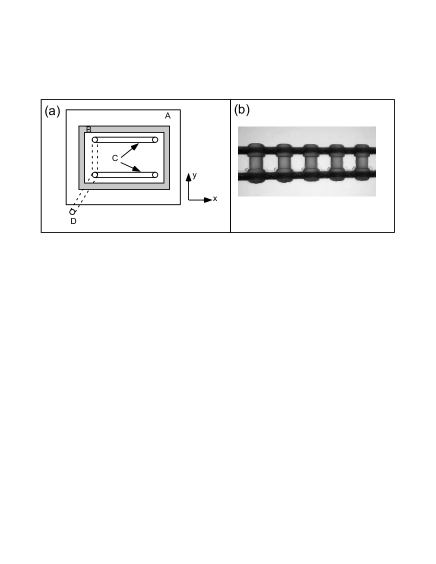
Figure 2: (a) A schematic of the apparatus as viewed from the top. The details are described in the text. Highlighted in the figure are the driving bands (C) that are used to generate flow. A close up photograph of a driving band is given in (b). The spacing for the bands is $4\ {\rm mm}$.

The bands that are used to drive the flow act as parallel walls moving at a constant speed. They are configured to move in opposite directions, ensuring a location (or region) of zero velocity in the flowing bubbles. To achieve a no-slip boundary conditions, belts with a groove spacing on the order of the average bubble size were used. The top of the belts are set at a height such that a single row of bubbles fits into the grooves on the belt.

For imaging the system, a standard CCD camera with a telephoto lens is used. The lens has a focal length of $6\ {\rm mm}$. The focus and the aperture are manually adjusted to optimize image quality by minimizing distortion and balancing the field of view with magnification of the bubbles. Images from the camera are directly digitized to the computer using a National Instruments frame grabber at a maximum frame rate of 30 frames/s. The actual frame rate was chosen based on the rate of strain to ensure the ability to track bubble motions. Selecting a frame rate that corresponded to a total applied strain of 0.001 between images was found to be adequate to track bubbles without an excessive overload on the number of images required to analyze sufficiently long total strains. This requirement combined with the rate of strain determined the frame rate for any given set of images.

The manufacture of the bubble rafts without a top is discussed in detail in Ref. Lauridsen et al. (2002). Essentially, a solution of $80\%$ of DI water, $15\%$ of glycerin and $5\%$ of a commercially available bubble solution (“Miracle bubbles” from Imperial Toy Corporation) by volume is used. Compressed nitrogen gas is flowed through the solution, with the flow rate and needle diameter controlling the size of the bubbles. By fixing the flow rate, we were able to generate essentially monodisperse systems. Without a top, the average diameter of the bubbles was $2.69\ {\rm mm}$, with a standard deviation of $0.09\ {\rm mm}$ based on fitting the bubble size distribution to a Gaussian. The bubble raft is stable for about two hours without significant popping. For producing the system with a top, the following procedure was used. A top plate, made from a 2 mm thick glass, is cleaned with a soap/water solution. Then, the glass is rinsed thoroughly with the same solution that constitutes the bubble raft in order to minimize the influence of any transient wetting or pinning dynamics. The top glass is placed on the Teflon frame, completely sealing the system. When making the bubbles, the top plate is moved to one end of the frame, creating a small opening on the other end. Bubbles are formed at the closed end, driving the bubbles towards the opening. When the bubbles fill the entire frame, the glass top is moved back into position to seal the system. Again, we used a monodisperse system. With a top, the average diameter of the bubbles was $2.43\ {\rm mm}$, with a standard deviation of $0.08\ {\rm mm}$ based on fitting the bubble size distribution to a Gaussian.

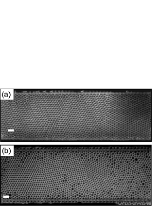
Figure 3: (a) Image of a typical set of bubbles in the case with no top on the system. The scale bar represents $7\ {\rm mm}$. (b) Image of a typical set of bubbles for the case of a top on the system. The scale bar represents $7\ {\rm mm}$.

Figure 3 shows a typical arrangement of the bubbles with and without the top. Both images include the bands used to drive the bubbles. One can see that the region outside the bands is filled with bubbles as well. One other difference between the two systems is the nature of bubbles well outside the bands. For the case of a top, because the system is effectively sealed, the bubbles fill the entire region within the supporting frame. For the case without a top, the flow outside the bands does show some unavoidable multilayer formation. This occurs in the corners of the Teflon frames. The loss of bubbles to these multilayers results in the formation of voids on the inner perimeter of the Teflon barriers. The density of bubbles between the bands, in the region of interest, is not noticeably affected by this. While the multilayers and void formation may have consequences for the pressure or stress fields globally, we find our velocity profiles and T1 rates/densities do not depend on the occurrence or growth of the multilayers or voids. We have checked for variation along the x-direction in many of the system properties due to the influence of the bubbles outside the flowing region. We observe a small entrance effect that decays rapidly. Therefore, we focus on the central area of the driven region.

III Analysis Methods

The primary dynamical features of the system we extract are the velocities of the individual bubbles and local topological rearrangements. The main topological event of concern for this paper are the T1 events, where neighbor rearrangements occur (see Fig. 1).

The raw data from the experiments consists of an image series capturing the time evolution of the bubbles at different rates of strain. The analysis of these images may be classified in two sections (1) A reduction of each image to a set of bubble centers, edges and vertices and (2) The evolution of these reduced measures between successive images to extract velocity profiles and T1 events.

The images are initially cropped to a desired region of interest and Fourier filtered to eliminate noise associated with the CCD camera and optical non-uniformities. The grayscale images are then reduced to binary images by thresholding them at an appropriate value to demarcate the interior regions of bubbles/cells from the bubble edges. The positions of the centers of each bubble are computed as the centers of mass of the interior regions of the cells in such a binary representation. This procedure reliably identifies over 99% of the bubbles in each image.

The center positions in consecutive images that show the least displacement are identified as being associated with the same bubbles. To reliably make such identification requires the displacement of the bubbles between successive images be less than their radii. This was one criteria used in selecting the frame rate. The velocity of the bubbles is computed using the displacement of the bubbles between two images and the time taken for the displacement and averaging over many bubbles and frames.

For the purposes of this paper, the velocity profiles represent an average over a total applied strain of 5 and a spatial average in the x-direction. The velocity profile is essentially independent of the x-position in most of the central region of the trough. There is a small entrance length at each end in which the velocity profile varies. Therefore, to be conservative, only the central 1/3 of the trough (in the x-direction) is used for computing average velocities. To confirm whether or not slip exists at the driving bands, we computed velocities for the entire width of the trough (in the y-direction). The y-direction is divided into evenly spaced bins, and all bubbles in a given y-bin, independent of their x position, are used to compute the average velocity at that point.

In our experiments, the the bubbles form densely packed two dimensional structures. We build a space filling tessellation from the positions of the cell centers using a Voronoi construction. The edges and vertices thus extracted are seen to accurately reproduce the network formed by the edges of individual cells in the bulk of the system. At the boundaries of the network, the Voronoi construction is not representative of the cell edges and therefore in any further analysis we expunge cells that have vertices at the boundaries.

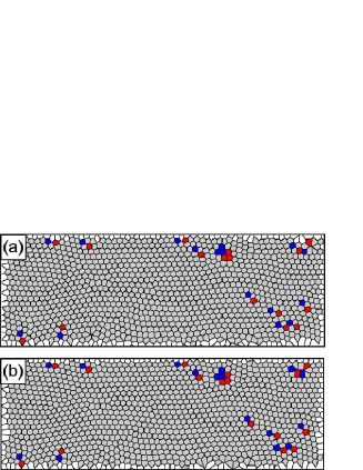
Figure 4: (color online) Illustration of identifying T1 events using the Voronoi construction. Image (a) and image (b) are the Voronoi reconstruction for two sequential images. Bubbles involved in T1 events are colored.

Knowing the vertices shared between cells makes it possible to identify cells that are neighbors of each other. In order to identify T1 events occurring in the system, we identify cells for which the next-nearest neighbors become nearest neighbors. This scheme identifies two of the cells that participate in a T1-event. The other two cells correspond to those in which nearest neighbors become next-nearest neighbors. While this methodology of identifies pairs of cells participating in T1 events, a number of such pairs often occur in proximity forming clusters that may be associated with slip zones. The size of these clusters seen depends on the framerate of image capture. However, assuming one had a sufficiently fast camera, all individual T1 events might be observed. The positions of the T1 events may be computed as the center of mass of the cells in each cluster. An example of the Voronoi reconstruction and detection of T1 events is given in Fig. 4. The two images illustrate the system before and after T1 events occur. Bubbles involved in the T1 events are shaded for easy identification.

The T1 events correspond to regions where slips between cells occur resulting in neighbor switching. These events are the primary mechanisms through which flows in foam systems are known to occur. The T1 events reflect a variation in the connectivity between neighboring cells from as a metric independent measure, while the velocity profiles of the bubbles are based on a eucledian metric. The relationship between the externally imposed shear inducing local T1 events and velocity profiles are explored in the next section.

IV Results

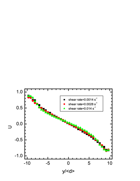
Figure 5: (color online) The scaled velocity profile ($U\equiv{\rm(bubble\ velocity)/(belt\ velocity)}$) as a function of scaled position ($y/<d>$) across the trough for three different rates of strain for a system without a top, where $<d>$ is the average bubble diameter. The scale of the position axis is set so that it extends from the edge of one belt to the other belt.

The main result of the paper is a comparison of Fig. 5 and Fig. 6. In both figures, three different scaled velocity profiles are plotted as a function of the displacement from the center of the trough in the y-direction (scaled by the average bubble diameter). (The velocity is scaled by the driving belt velocity, $U\equiv{\rm(bubble\ velocity)/(belt\ velocity)}$.) A few common features of the velocity profiles are worth highlighting. If there is no slip at the boundary, the scaled velocity should be one by definition. Second, the velocities scale for both boundary conditions and the three rates of strain reported on here. This indicates that we are in a rate independent regime QUA . Finally, because the bands are moving in opposite directions, the velocity goes through zero, and it is expected to be zero in the center of the trough. Both profiles are consistent with this expectation.

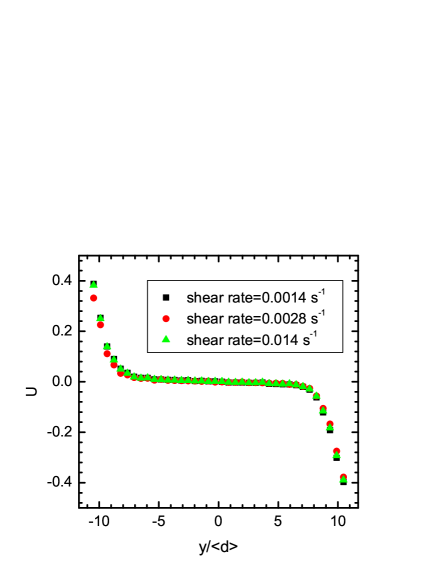
Figure 6: (color online) The scaled velocity profile ($U\equiv{\rm(bubble\ velocity)/(belt\ velocity)}$) as a function of scaled position ($y/<d>$) across the trough for three different rates of strain for a system with a top, where $<d>$ is the average bubble diameter. The scale of the position axis is set so that it extends from the edge of one belt to the other belt.

The most striking feature is the extreme localization of the flow when there is a top (Fig. 6) and the corresponding essentially linear profile without a top (Fig. 5). This provides strong evidence for the importance of accounting for the confining boundary conditions, even in a case where one expects the rate of strain to be sufficiently slow. For comparison with earlier work, the data with a top is plotted semi-log in Fig. 7. One can see that the behavior near each boundary is consistent with an exponential decay over a few bubble diameters. The deviations from the exponential behavior in the center may be in part due to the experimental resolution of our velocity measurements. Also, it should be noted that the profile in the case with no top (Fig. 5) is not perfectly linear, as would be expected for a “simple” fluid. One candidate for the deviations from linearity is the monodispersity of the bubble raft. This is certainly an interesting question, and will be the subject of future more detailed work. However, for the purposes of establishing the impact of the boundaries, the difference between the profiles in Fig. 5 and Fig. 6 are more important than the variations from linear velocity in the case of not having a top.

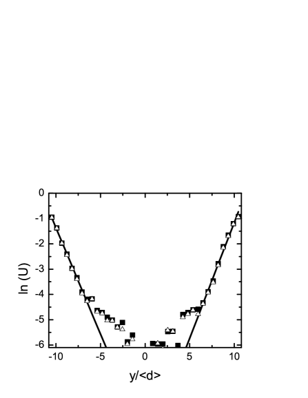
Figure 7: The natural log of the scaled velocity profile ($\ln(U)$) as a function of scaled position ($y/<d>$) across the trough for two rates of strain in the system with a top (solid squares are a rate of strain of $0.014\ {\rm s^{-1}}$ and open triangles are $0.0014\ {\rm s^{-1}}$.) The lines represent linear fits to the $0.014\ {\rm s^{-1}}$ data, indicating an exponential decay of the velocity in that regime.

The other feature of the flow that is apparent is the behavior at the driving band. In the case of no top, we achieved a no-slip boundary condition by containing the bubbles in the spaces in the bands. We tested this by varying the position of the band relative to the bubbles. If the height of the band was such that the bubbles sat at the edge of a band but not in one of the gaps, we observed complete slip at the boundary. In this case, no flow was observed anywhere in the system. For the case with the top, we observed some slip at the boundary. However, the “slip” was not complete in the sense that the bands were still able to drive flow, just with a reduced average speed relative to the speed of the bands. The introduction of slip in the case of the top is most likely the result of the drag from the top acting on the bubbles. An interesting feature of the slip is that the degree of slip was independent of the rate of strain. This suggests that both the force between the bubbles and the driving band and the drag of the plate on the bubbles are independent of rate of strain. One could test the impact of the plate in the future by selecting driving bands with varying degrees of interaction between the band and the bubbles. For a sufficiently strong interaction, one would expect no slip, despite the drag due to the plate.

Figure 8: Positions of T1 events in the central portion of the system (a fraction of the $x$ direction) without a confining top. Both the $x$ and $y$ position is scaled by the average bubble diameter $<d>$.

To further explore the impact of the confining top boundary, Fig. 8 and 9 compare the spatial distribution of T1 events. For these plots, only a total applied strain of 0.5 is used. (The smaller interval of strain is used to avoid overcrowding the plot.) To ensure that the steady state statistics are being viewed, the last 0.5 of strain out of a total strain of 5 is selected. Because we are interested in the differences of the boundary conditions at the slowest possible rate of strain, only the case for $\dot{\gamma}=1.4\times 10^{-3}\ {\rm s^{-1}}$ is shown. Each circle represents the spatial location of a T1 event.

Figure 9: Positions of T1 events in the central portion of the system (a fraction of the $x$ direction) without a confining top. Both the $x$ and $y$ position is scaled by the average bubble diameter $<d>$.

The most dramatic feature is the absence of T1 events from the center region when a top is placed on the system. This is highlighted in Fig. 10 where the probability of a T1 event occurring at a particular $y/<d>$ position in the range $-22\leq x/<d>\ \leq 22$. The histogram illustrates the dramatic difference between the number of T1 events in the central portion of the system for the two cases. This indicates the strong connection between the occurrence of T1 events and the existence of non-zero velocity. Also of interest, is the slight increase of T1 events near the boundaries that results in a peak in the probability for both cases. The peak is close to the boundary, and more pronounced for the case with the top. The nature of the peaks reinforces the relative boundary slip for the two cases, as the probability of T1 events right at the boundary drops to zero for the case without a top, confirming a lack of slip. In contrast, with the top, some percentage of T1 events occur even very close to the boundary, as must happen if slip occurs.

A noteworthy feature of the distribution of T1 events is the intermittent occurrence of coherent events along lines throughout the system. These structures appear as lines in Fig. 8 and correspond to relaxation through a number of neighbor rearrangements resulting in large scale slip zones within the bubble raft. (Various views of a three-dimensional space-time plot of the occurrence of T1 events is available on EPAPS T1C that illustrates the temporal correlations between events.) Preliminary results with a high-speed camera suggests that the chains of T1 events align with the crystallographic axes of the bubble lattice, but more systematic work is necessary to confirm this correlation. Also, it is interesting to speculate on the correlation between these apparent “slip planes” in which the majority of T1 events occur and the observed systematic variation in the velocity profile from linear (see Fig. 5). Clearly, future work is needed to both clarify the impact of monodispersity on the degree of linearity of the velocity profile and to explore more quantitatively the connection between T1 events and velocity profiles.

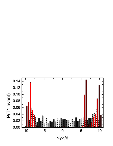
Figure 10: (Color online) Histogram of the probability of a T1 event (P(T1 event)) as a function of $y/<d>$ computed using in the range $-22\leq x/<d>\ \leq 22$ for both the case with a top (solid red bars) and without a top (hashed open bars). The histogram shows the absence of T1 events from the center of the system with a top present, and the relative flatness of the distribution in the center for flow without a top.

In summary, our results demonstrate that for otherwise identical systems under conditions of small applied rates of strain, the existence of a confining solid plate can have a dramatic impact on the flow behavior of the system by suppressing flow in most of the system. The suppression of flow is paralleled by a suppression of T1 events, confirming the expected strong connection between the two processes. This strongly suggests that even when there is evidence of rate independence (for example, the scaling of velocity profiles as seen in this paper), one has to be very careful in interpreting the measurements from a system with a top in place.

In trying to understand the role of the top plate, the results point to three primary sources of damping for the bubble rafts considered. These correspond to viscous drag between (a) bubbles, (b) bubbles and the water subphase and (c) bubbles and the glass top plate (Fig. 6) or air (Fig. 5). The bubble-bubble interaction can be considered to be the “intrinsic” dissipation that provides the effective viscosity for the system under flow. Previous experiments indicate that the bubble-bubble interactions are significantly stronger than any bubble-subphase interaction Lauridsen et al. (2004). The velocity profiles indicate the relative strength between (a) and (c). With a top, the exponential decay of velocity at the boundaries (Fig 7) suggests that the viscous damping between the bubbles and the top glass plate dominates relative to the bubble-bubble interactions, resulting in an exponential profile. Under the current conditions, without a top, the bubble-bubble interactions produce a velocity profile that is consistent with a model that treats the foam as a viscous fluid, even if the viscosity is non-Newtonian. What remains to be seen is under what, if any, conditions the velocity profile in the linear case exhibits significant departures from linear. For example, at sufficiently slow rates of strain or for larger system sizes, new behavior may be observed. Finally, it should be noted that recent work on a system of only two bubbles connects these differences to whether or not a system is modelled as a dry foam (confining plates) or a wet foam (bubble raft without a top) Vaz and Cox (2005), which can also be connected with the different mechanisms of dissipation. This is an interesting connection that requires further exploration in the large system.