Complex-temperature phase diagram
of Potts and RSOS models

Abstract

We study the phase diagram of $Q$-state Potts models, for $Q=4\cos^{2}(\pi/p)$ a Beraha number ($p>2$ integer), in the complex-temperature plane. The models are defined on $L\times N$ strips of the square or triangular lattice, with boundary conditions on the Potts spins that are periodic in the longitudinal ($N$) direction and free or fixed in the transverse ($L$) direction. The relevant partition functions can then be computed as sums over partition functions of an $A_{p-1}$ type RSOS model, thus making contact with the theory of quantum groups. We compute the accumulation sets, as $N\to\infty$, of partition function zeros for $p=4,5,6,\infty$ and $L=2,3,4$ and study selected features for $p>6$ and/or $L>4$. This information enables us to formulate several conjectures about the thermodynamic limit, $L\to\infty$, of these accumulation sets. The resulting phase diagrams are quite different from those of the generic case (irrational $p$). For free transverse boundary conditions, the partition function zeros are found to be dense in large parts of the complex plane, even for the Ising model ($p=4$). We show how this feature is modified by taking fixed transverse boundary conditions.

Key Words: Potts model, RSOS model, Beraha number, limiting curve, quantum groups

1 Introduction

The $Q$-state Potts model [1, 2] can be defined for general $Q$ by using the Fortuin–Kasteleyn (FK) representation [3, 4]. The partition function $Z_{G}(Q;v)$ is a polynomial in the variables $Q$ and $v$. This latter variable is related to the Potts model coupling constant $J$ as

$$v\;=\;e^{J}-1.$$ (1.1)

It turns out useful to define the temperature parameter $x$ as

$$x\;=\;\frac{v}{\sqrt{Q}}$$ (1.2)

and to parameterize the interval $Q\in(0,4]$ as

$$Q\;=\;4\cos^{2}\left(\frac{\pi}{p}\right)\,,\qquad p\in(2,\infty].$$ (1.3)

For generic values of $Q$, the main features of the phase diagram of the Potts model in the real $(Q,x)$-plane have been known for many years [2, 5]. It contains in particular a curve $x_{\rm FM}(Q)>0$ of ferromagnetic phase transitions which are second-order in the range $0<Q\leq 4$, the thermal operator being relevant. The analytic continuation of the curve $x_{\rm FM}(Q)$ into the antiferromagnetic regime yields a second critical curve $x_{\rm BK}(Q)<0$ with $0<Q<4$ along which the thermal operator is irrelevant. Therefore, for a fixed value of $Q$, the critical point $x_{\rm BK}(Q)$ acts as the renormalization group (RG) attractor of a finite range of $x$ values: this is the Berker-Kadanoff (BK) phase [6, 7].

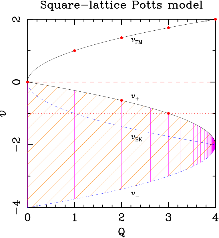
Figure 1: Generic phase diagram for the two-dimensional Potts model in the $(Q,v)$-plane. The solid black curve in the ferromagnetic ($v>0$) region shows the standard ferromagnetic phase transition curve $v_{\rm FM}(Q)$, and the blue dashed curve is its analytic continuation $v_{\rm BK}(Q)$ into the antiferromagnetic region. This latter curve acts as an RG attractor for the Berker-Kadanoff phase (the orange hatched region). This is separated from the limit of infinite temperature (red dashed curve) by the antiferromagnetic phase-transition curve $v_{+}(Q)$ (solid black curve in the $v<0$ region), and from the $v\to-\infty$ limit by its counterpart $v_{-}(Q)$ (dot-dashed blue curve). The red horizontal dotted curve represents the zero-temperature antiferromagnet ($v=-1$). The pink vertical lines show the Beraha numbers $Q=4\cos^{2}(\pi/p)$ ($p=2,3,\ldots$): the phase diagram on these lines is different from the generic one shown here and forms the object of the present article. Note that the exact functional forms of the curves $v_{\rm FM}(Q)$, $v_{\rm BK}(Q)$, and $v_{\pm}(Q)$ are lattice-dependent; the figure shows their explicit forms for the square-lattice model.

The generic phase diagram is shown in Fig. 1. Since the infinite-temperature limit ($x=0$) and the zero-temperature ferromagnet ($|x|=\infty$) are of course RG attractive, consistency of the phase diagram requires that the BK phase be separated from these by a pair of RG repulsive curves $x_{\pm}(Q)<0$. The curve $x_{+}(Q)$ is expected to correspond to the antiferromagnetic (AF) phase transition of the model [8].

The above scenario thus essentially relies on the RG attractive nature of the curve $x_{\rm BK}(Q)$, and since this can be derived [5] from very general Coulomb gas considerations, the whole picture should hold for any two-dimensional lattice. But it remains of course of great interest to compute the exact functional forms of the curves $x_{\rm FM}(Q)$, $x_{\rm BK}(Q)$, and $x_{\pm}(Q)$—and the corresponding free energies—for specific lattices.

The square-lattice Potts model is the best understood case. Here, Baxter [2, 9] has found the exact free energy along several curves $x=x_{\rm c}(Q)$:

$$x_{\rm c}(Q)\;=\;\begin{cases}+1&\qquad\text{(FM)}\\ -\frac{2}{\sqrt{Q}}+\sqrt{\frac{4-Q}{Q}}&\qquad\text{(AF)}\\ -1&\qquad\text{(BK)}\\ -\frac{2}{\sqrt{Q}}-\sqrt{\frac{4-Q}{Q}}&\qquad\text{(AF)}\end{cases}$$ (1.4)

where $x_{\rm c}=1$ and $x_{\rm c}=-1$ can be identified respectively with $x_{\rm FM}(Q)$ and $x_{\rm BK}(Q)$. The curves $x_{\pm}=-2/\sqrt{Q}\pm\sqrt{(4-Q)/Q}$ are mutually dual (and hence equivalent) curves of AF phase transitions, which are again second-order in the range $0<Q\leq 4$. These curves also form the boundaries of the $x$-values controlled by the BK fixed point [7], as outlined above. Note that the four points $x_{\rm c}(q)$ in Eq. (1.4) correspond to the points where the circles

$$|x|&=1\\ \left|x+\frac{2}{\sqrt{Q}}\right|=\sqrt{\frac{4-Q}{Q}}$$ (1.5)

cross the real $x$-axis. These two circles intersect at the points

$$x\;=\;-e^{\pm i\,\pi/p}$$ (1.6)

which will be shown below to play a particular role in the phase diagram (see Conjecture 4.1.1).

In the case of a triangular lattice, Baxter and collaborators [10, 11, 12] have found the free energy of the Potts model along the curves

$$\sqrt{Q}x^{3}+3x^{2}&=1\,,\\ x=-\frac{1}{\sqrt{Q}}\,.$$ (1.7)

The upper branch of Eq. (1.7a) is identified with the ferromagnetic critical curve $x_{\text{FM}}(Q)$. We have numerical evidence that the middle and lower branches correspond respectively to $x_{\text{BK}}(Q)$ and $x_{-}(Q)$, the lower boundary of the BK phase. The position of $x_{+}(Q)$, the upper branch of the BK phase, is at present unknown [13] (but see Ref. [14] for the $Q\to 0$ limit). Along the line (1.7b) the Potts model reduces to a coloring problem, and the partition function is here known as the chromatic polynomial. The line (1.7b) belongs to the RG basin of the BK phase for $0<Q<2+\sqrt{3}$ [15].

The critical properties—still with $Q$ taking generic values—for these two lattices are to a large extent universal. This is not so surprising, since the critical exponents can largely be obtained by Coulomb gas techniques (although the antiferromagnetic transition still reserves some challenges [8]). Thus, there is numerical evidence that the exponents along the curves $x_{\text{FM}}(Q)$, $x_{\text{BK}}(Q)$ and $x_{-}(Q)$ coincide, whereas the evidence for the curve $x_{+}(Q)$ is non-conclusive [14]. On the other hand, on the less-studied triangular lattice we cannot yet exclude the possible existence of other curves of second-order phase transitions that have no counterpart on the square lattice.

But in general we can only expect universality to hold when the Boltzmann weights in the FK representation are non-negative (i.e., for $Q\geq 0$, $v\geq 0$), or when the parameter $p$ takes generic (i.e., irrational) values. The present paper aims at studying the situation when $p$ takes non-generic values; for simplicity we limit ourselves to the case of integer $p>2$. The number of spin states is then equal to a so-called Beraha number $B_{p}$

$$Q\;=\;B_{p}\;=\;4\cos^{2}\left(\frac{\pi}{p}\right)\,,\qquad p=3,4,5,\ldots.$$ (1.8)

The special physics at rational values of $p$ is intimately linked to the representation theory of the quantum group $U_{q}(SU(2))$, the commutant of the Temperley-Lieb algebra, when the deformation parameter $q$ is a root of unity. As we shall review in Section 2 below, the quantum group symmetry of the Potts model at rational $p$ implies that many eigenvalues of the transfer matrix in the FK representation have zero amplitude or cancel in pairs because of opposite amplitudes; these eigenvalues therefore become spurious and do not contribute to the partition function [6, 7].

Remarkably, for $p$ integer and $x$ inside the BK phase, even the leading eigenvalue acquires zero amplitude. Moreover, all the eigenvalues which scale like the leading one in the thermodynamic limit vanish from the partition function, and so, even the bulk free energy $f(p;x)$ is modified [8]. In other words, $f(p;x)$ experiences a singularity whenever $p$ passes through an integer value. This means in particular that for $p$ integer the critical behavior can either disappear, or be modified, or new critical points (and other non-critical fixed points) can emerge.

For the sake of clarity, we discuss the simplest example of this phenomenon. Consider, on the square lattice, on one hand the $Q\to 2$ state model (i.e., with $Q$ tending to 2 through irrational values of $p$) and on the other the $Q=2$ Ising model (i.e., with fixed integer $p=4$). For the former case, the generic phase diagram and the associated RG flows are shown in the top part of Fig. 2. The three critical points $x_{\rm FM}$ and $x_{\pm}$ have central charge $c=1/2$, while the fourth one $x_{\rm BK}$ has $c=-25/2$. For the latter case, new non-critical fixed points appear (by applying the duality and $Z_{2}$ gauge symmetries to the one at $x=0$), and the RG flows become as shown in the bottom part of Fig. 2. One now has $c=1/2$ for all four critical fixed points. (We shall treat the Ising model in more detail in Section 7.1 below.)

By contrast to the universality brought out for generic $Q$, the phase diagram and critical behavior for integer $p$ is likely to have lattice dependent features. Let us give a couple of examples of this non-universality. The zero-temperature triangular-lattice Ising antiferromagnet, $(Q,v)=(2,-1)$, is critical and becomes in the scaling limit a free Gaussian field with central charge $c=1$ [16, 17, 18], whereas the corresponding square-lattice model is non-critical, its partition function being trivially $Z=2$. While this observation does not in itself imply non-universality, since the critical temperature is expected to be lattice dependent (as is the value of $x_{\rm FM}(Q)$), the point to be noticed is that for no value of $v$ does the $Q=2$ square-lattice model exhibit $c=1$ critical behavior. In the same vein, the square-lattice Potts model with $(Q,v)=(3,-1)$ is equivalent to a critical six-vertex model (at $\Delta=1/2$) [19, 20], with again $c=1$ in the scaling limit, whereas now the corresponding triangular-lattice model is trivial ($Z=3$). Now, the triangular-lattice model does in fact exhibit $c=1$ behavior elsewhere (for $x=x_{-}$), but the compactification radius is different from that of the square-lattice theory and accordingly the critical exponents differ. Finally, $(Q,v)=(4,-1)$ is a critical $c=2$ theory on the triangular lattice [21, 22], but is non-critical on the square lattice [23].

Because of the eigenvalue cancellation scenario sketched above, the FK representation is not well suited for studying the Potts model at integer $p$. Fortunately, for $Q=B_{p}$ there exists another representation of the Potts model, in terms of an RSOS model of the $A_{p-1}$ type [24], in which the cancellation phenomenon is explicitly built-in, in the sense that for generic values of $x$ all the RSOS eigenvalues contribute to the partition function. On the square lattice, the RSOS model has been studied in great detail [25, 26, 24, 27] at the point $x=x_{\rm FM}=1$, where the model happens to be homogeneous. Only very recently has the case of general real $x\neq 1$ (where the RSOS model is staggered, i.e., its Boltzmann weights are sublattice dependent) attracted some attention [8], and no previous investigation of other lattices (such as the triangular lattice included in the present study) appears to exist.

The very existence of the RSOS representation has profound links [27, 28] to the representation theory of the quantum group $U_{q}(SU(2))$ where the deformation parameter $q$ defined by

$$Q=\left(q+q^{-1}\right)^{2}=B_{p}\,,\qquad q=\exp(i\pi/p)\,,$$ (1.9)

is a root of unity. To ensure the quantum group invariance one needs to impose periodic boundary conditions along the transfer direction. Further, to ensure the exact equivalence between Potts and RSOS model partition functions the transverse boundary conditions must be non-periodic. For definiteness we shall therefore study square- or triangular-lattice strips of size $L\times N$ spins, with periodic boundary conditions in the $N$-direction. The boundary conditions in the $L$-direction are initially taken as free, but we shall later consider fixed transverse boundary conditions as well. For simplicity we shall henceforth refer to these boundary conditions as free cyclic and fixed cyclic.

Using the RSOS representation we here study the phase diagram of the Potts model at $Q=B_{p}$ through the loci of partition function zeros in the complex $x$-plane. According to the Beraha-Kahane-Weiss theorem [30], when $N\to\infty$, the accumulation points of these zeros form either isolated limiting points (when the amplitude of the dominant eigenvalue vanishes) or continuous limiting curves $\mathcal{B}_{L}$ (when two or more dominant eigenvalues become equimodular); we refer to Ref. [32] for further details. In the RSOS representation only the latter scenario is possible, since all amplitudes are strictly positive. As usual in such studies, branches of $\mathcal{B}_{L}$ that traverse the real $x$-axis for finite $L$, or “pinch” it asymptotically in the thermodynamic limit $L\to\infty$, signal the existence of a phase transition. Moreover, the finite-size effects and the impact angles [33] give information about the nature of the transition.

The limiting curves $\mathcal{B}_{L}$ constitute the boundaries between the different phases of the model. Moreover, in the present set-up, each phase can be characterized topologically by the value of the conserved quantum group spin $S_{z}$, whose precise definition will be recalled in Section 2 below. (A similar characterization of phases of the chromatic polynomial was recently exploited in Ref. [34], but in the FK representation). One may think of $S_{z}$ as a kind of “quantum” order parameter. A naive entropic reasoning would seem to imply that for any real $x$ the ground state (free energy) has $S_{z}=0$, since the corresponding sector of the transfer matrix has the largest dimension. It is a most remarkable fact that large portions of the phase diagram turn out have $S_{z}\neq 0$.

We have computed the limiting curves $\mathcal{B}_{L}$ in the complex $x$-plane completely for $p=4,5,6,\infty$ and $L=2,3,4$ for both lattices. Moreover, we have studied selected features thereof for $p>6$ and/or $L>4$. This enables us to formulate several conjectures about the topology of $\mathcal{B}_{L}$ which are presumably valid for any $L$, and therefore, provides information about the thermodynamic limit $L\to\infty$. The resulting knowledge is a starting point for gaining a better understanding of the fixed point structure and renormalization group flows in these Potts models.

Our work has been motivated in particular by the following open issues:

1. As outlined above, the eigenvalue cancellation phenomenon arising from the quantum group symmetry at integer $p$ modifies the bulk free energy in the Berker-Kadanoff phase. For the Ising model we have seen that this changes the RG nature (from attractive to repulsive) of the point $x_{\rm BK}$ as well as its critical exponents (from $c=-25/2$ to $c=1/2$). But for general integer $p$ it is not clear whether $x_{\rm BK}$ will remain a phase transition point, and assuming this to be the case what would be its properties.

2. The chromatic line $x=-1/\sqrt{Q}$ does not appear to play any particular role in the generic phase diagram of the square-lattice model. By contrast, it is an integrable line [11, 12] for the generic triangular-lattice model. Qua its role as the zero-temperature antiferromagnet one could however expect the chromatic line to lead to particular (and possibly critical) behavior in the RSOS model. Even when critical behavior exists in the generic case (e.g., on the triangular lattice) the nature of the transition may change when going to the case of integer $p$ (e.g., from $c=-25/2$ for the $Q\to 2$ model to $c=1$ for the zero-temperature Ising antiferromagnet).

3. Some features in the antiferromagnetic region might possibly exhibit an extreme dependence on the boundary conditions, in line with what is known, e.g., for the six-vertex model. It is thus of interest to study both free and fixed boundary conditions. To give but one example of what may be expected, we have discovered—rather surprisingly—that with free cyclic boundary conditions the partition function zeros are actually dense in substantial parts of the complex plane: this is true even for the simplest case of the square-lattice Ising model.

4. A recent numerical study [8] of the effective central charge of the RSOS model with periodic boundary conditions, as a function of $x$, has revealed the presence of new critical points inside the BK phase. In particular, strong evidence was given for a physical realization of the integrable flow [35] from parafermion to minimal models. The question arises what would be the location of these new points in the phase diagram.

5. In the generic case, the spin $S_{z}$ of the ground state may be driven to arbitrary large values upon approching the point $(Q,x)=(4,-1)$ from within the BK phase [7, 34]. Is a similar mechanism at play for integer $p$?

The paper is organized as follows. In Section 2 we introduce the RSOS models and describe their precise relationship to the Potts model, largely following Refs. [24, 27, 28]. We then present, in Section 3, the limiting curves found for the square-lattice model with free cyclic boundary conditions, leading to the formulation of several conjectures in Section 4. Sections 5–6 repeat this programme for the triangular-lattice model. In Section 7 we discuss the results for free cyclic boundary conditions, with special emphasis on the thermodynamic limit, and motivate the need to study also fixed cyclic boundary conditions. This is then done in Sections 8–9. Finally, Section 10 is devoted to our conclusions. An appendix gives some technical details on the dimensions of the transfer matrices used.

2 RSOS representation of the Potts model

The partition function of the two-dimensional Potts model can be written in several equivalent ways, though sometimes with different domains of validity of the relevant parameters (notably $Q$). The interplay between these different representations is at the heart of the phenomena we wish to study.

The spin representation for $Q$ integer is well-known. Its low-temperature expansion gives the FK representation [3, 4] discussed in the Introduction, where $Q$ is now an arbitrary complex number. The (interior and exterior) boundaries of the FK clusters, which live on the medial lattice, yield the equivalent loop representation with weight $Q^{1/2}$ per loop.

An oriented loop representation is obtained by independently assigning an orientation to each loop, with weight $q$ (resp. $q^{-1}$) for counterclockwise (resp. clockwise) loops, cf. Eq. (1.9). In this representation one can define the spin $S_{z}$ along the transfer direction (with parallel/antiparallel loops contributing $\pm 1/2$) which acts as a conserved quantum number. Note that $S_{z}=j$ means that there are at least $j$ non-contractible loops, i.e., loops that wind around the periodic ($N$) direction of the lattice. The weights $q^{\pm 1}$ can be further redistributed locally, as a factor of $q^{\alpha/2\pi}$ for a counterclockwise turn through an angle $\alpha$ [2]. While this redistribution correctly weights contractible loops, the non-contractible loops are given weight $2$, but this can be corrected by twisting the model, i.e., by inserting the operator $q^{S_{z}}$ into the trace that defines the partition function.

A partial resummation over the oriented-loop splittings at vertices which are compatible with a given orientation of the edges incident to that vertex now gives a six-vertex model representation [36]. Each edge of the medial lattice then carries an arrow, and these arrows are conserved at the vertices: the net arrow flux defines $S_{z}$ as before. The six-vertex model again needs twisting by the operator $q^{S_{z}}$ to ensure the correct weighing in the $S_{z}\neq 0$ sectors. The Hamiltonian of the corresponding spin chain can be extracted by taking the anisotropic limit, and is useful for studying the model with the Bethe Ansatz technique [2]. The fact that this Hamiltonian commutes with the generators of the quantum group $U_{q}(SU(2))$ links up with the nice results of Saleur and coworkers [27, 28, 6, 7].

Finally, the RSOS representation [24, 27, 28] emerges from a certain simplification of the above representations when $q=\exp(i\pi/p)$ is a root of unity (see below).

All these formulations of the Potts model can be conveniently studied through the corresponding transfer matrix spectra: these give access to the limiting curves $\mathcal{B}_{L}$, correlation functions, critical exponents, etc.

In the FK representation the transfer matrix ${\mathsf{T}}_{\text{FK}}^{(2)}(L)$ is written in a basis of connectivities (set partitions) between two time slices of the lattice (see Ref. [34] for details), and the transfer matrix propagates just one of the time slices. Each independent connection between the two slices is called a bridge; the number of bridges $j$ is a semi-conserved quantum number in the sense that it cannot increase upon action of the transfer matrix. The bridges serve to correctly weight the clusters that are non-contractible with respect to the cyclic boundary conditions. This is accomplished by writing the partition function as

$$Z_{\text{FK}}=\langle f|{\mathsf{T}}_{\text{FK}}^{(2)}(L)^{N}|i\rangle=\sum_{i\geq 1}\alpha_{i}\,\lambda^{N}_{i}$$ (2.1)

for suitable initial and final vectors $|i\rangle$ and $\langle f|$. The vector $|i\rangle$ identifies the two time slices, while $\langle f|$ imposes the periodic boundary conditions (it “reglues” the time slices) and weighs the resulting non-contractible clusters. Note that these vectors conspire to multiply the contribution of each eigenvalue $\lambda_{i}$ by an amplitude $\alpha_{i}=\alpha_{i}(Q)$: this amplitude may vanish for certain values of $Q$.

On the other hand, in the six-vertex representation the transfer matrix is written in the purely local basis of arrows, whence the partition function can be obtained as a trace (which however has to be twisted by inserting $q^{S_{z}}$ as described above). But even without the twist the eigenvalues are still associated with non-trivial amplitudes, as we now review.

Let us consider first a generic value of $q$, i.e., an irrational value of $p$. The $U_{q}(SU(2))$ symmetry of the spin chain Hamiltonian implies that one can classify eigenvalues according to their value $j$ of $S_{z}$, and consider only highest weights of spin $j$. Define now $K_{1,2j+1}(p,L;x)$ as the generating function of the highest weights of spin $j$, for given values of $p$, $L$ and $x$. The partition function of the untwisted six-vertex model with the spin $S$ (not $S_{z}$) fixed to $j$ is therefore $(2j+1)\,K_{1,2j+1}(p,L;x)$. Imposing the twist, the corresponding contribution to the partition function of the Potts model becomes $S_{j}(p)\,K_{1,2j+1}(p,L;x)$, where the $q$-deformed number $S_{j}(p)\equiv(2j+1)_{q}$ is defined as follows

$$S_{j}(p)\;=\;\frac{\sin(\pi(2j+1)/p)}{\sin(\pi/p)}\,.$$ (2.2)

$S$ has a simple interpretation in the FK representation as the number of bridges, whereas it is $S_{z}$ which has a simple interpretation in the six-vertex model representation as the conserved current.

Different representations correspond to choosing different basis states: a given cluster state is an eigenvector of $S$, but not $S_{z}$, and a given vertex state is an eigenvector of $S_{z}$, but not $S$. The eigenvectors of the Hamiltonian are eigenvectors of both $S$ and $S_{z}$, and are thus combinations of vertex states (or of cluster states if one works in the FK representation). But note that the dimensions of the transfer matrix are not exactly the same in the vertex and the FK representations, as the $2j+1$ possible values of $S_{z}$ for a given $S=j$ are not taken into account in the same way: in the vertex representation, it corresponds to a degeneracy of the eigenvalues, whereas in the FK representation it appears because of the initial and final vectors which sandwich the transfer matrix in Eq. (2.1).

The total partition function of the $Q$-state Potts model on a strip of size $L_{\text{F}}\times N_{\text{P}}$ can therefore be exactly written as [24, 27, 28]

$$Z_{L_{\text{F}}\times N_{\text{P}}}(Q;v)\;=\;Q^{LN/2}\sum_{j=0}^{L}S_{j}(p)\,K_{1,2j+1}(p,L;x)$$ (2.3)

Note that the summation is for $0\leq j\leq L$, as the maximum number of bridges is equal to the strip width $L$.

For $p$ rational, Eq. (2.3) is still correct, but can be considerably simplified. In the context of this paper we only consider the simplest case of $p$ integer. Indeed, note that using Eq. (2.2), we obtain that, for any integer $n$,

$$S_{(n+1)p-1-j}(p)&=-S_{j}(p)\\ S_{np+j}(p)=S_{j}(p)\,.$$ (2.4)

Therefore, after factorization, Eq. (2.3) can be rewritten as

$$Z_{L_{\text{F}}\times N_{\text{P}}}(Q;v)\;=\;Q^{LN/2}\sum_{j=0}^{\lfloor(p-2)/2\rfloor}S_{j}(p)\,\chi_{1,2j+1}(p,L;x)\,,$$ (2.5)

where

$$\chi_{1,2j+1}(p,L;x)\;=\;\sum_{n\geq 0}\left[K_{1,2(np+j)+1}(p,L;x)-K_{1,2((n+1)p-1-j)+1}(p,L;x)\right]\,.$$ (2.6)

For convenience in writing Eq. (2.6) we have defined $K_{1,2j+1}(p,L;x)\equiv 0$ for $j>L$. Note that the summation in Eq. (2.5) is now for $0\leq j\leq\lfloor(p-2)/2\rfloor$. Furthermore, $\chi_{1,2j+1}(p,L;x)$ is a lot simpler that it seems. Indeed, when $p$ is integer, the representations of $U_{q}(SU(2))$ mix different values of $j$ related precisely by the transformations $j\to j+np$ and $j\to(n+1)p-1-j$ [cf. Eq. (2.4)]. Therefore, a lot of eigenvalues cancel each other in Eq. (2.6). This is exactly why the transfer matrix in the FK representation contains spurious eigenvalues, and is not adapted to the case of $p$ integer.

The representation adapted to the case of $p$ integer is the so-called RSOS representation. It can be proved that $\chi_{1,2j+1}$ is the partition function of an RSOS model of the $A_{p-1}$ type [24] with given boundary conditions [27] (see below). In this model, heights $h_{i}=1,2,\ldots,p-1$ are defined on the union of vertices and dual vertices of the original Potts spin lattice. Neighboring heights are restricted to differ by $\pm 1$ (whence the name RSOS = restricted solid-on-solid). The boundary conditions on the heights are still periodic in the longitudinal direction, but fixed in the transverse direction. More precisely, the cyclic strip $L_{\rm F}\times N_{\rm P}$ has precisely two exterior dual vertices, whose heights are fixed to $1$ and $2j+1$ respectively. It is convenient to draw the lattice of heights as in Figures 3–4 (showing respectively a square and a triangular-lattice strip of width $L=2$), i.e., with $N$ exterior vertices above the upper rim, and $N$ exterior vertices below the lower rim of the strip: all these exterior vertices close to a given rim are then meant to be identified.

For a given lattice of spins, the weights of the RSOS model are most easily defined by building up the height lattice face by face, using a transfer matrix. The transfer matrix adding one face at position $i$ is denoted $H_{i}=xI_{i}+e_{i}$ (resp. $V_{i}=I_{i}+xe_{i}$) if it propagates a height $h_{i}\to h^{\prime}_{i}$ standing on a direct (resp. a dual) vertex, where $I_{i}=\delta(h_{i},h^{\prime}_{i})$ is the identity operator, and $e_{i}$ is the Temperley-Lieb generator in the RSOS representation [24]:

$$e_{i}=\delta(h_{i-1},h_{i+1})\frac{\left[\sin(\pi h_{j}/p)\sin(\pi h^{\prime}_{j}/p)\right]^{1/2}}{\sin(\pi h_{j-1}/p)}\,.$$ (2.7)

Note that all the amplitudes $S_{j}(p)$ entering in Eq. (2.5) are strictly positive. Therefore, for a generic value of the temperature $x$, all the eigenvalues associated with $\chi_{1,2j+1}(p,L;x)$ for $0<2j+1<p$ contribute to the partition function. This is the very reason why we use the RSOS representation. Recall that there are analogous results in conformal field theory [37]. In fact, for $x$ equal to $x_{\rm FM}(Q)$ and in the continuum limit, $K_{1,2j+1}$ corresponds to the generating function of a generic representation of the conformal symmetry with Kac-table indices $r=1$ and $s=2j+1$, whereas $\chi_{1,2j+1}$ corresponds to the generating function (character) of a minimal model. Thus, Eq. (2.6) corresponds to the Rocha-Caridi equation [38], which consists of taking into account the null states. One could say that the FK representation does not identify all the states differing by null states, whereas the RSOS representation does. Therefore, the dimension of the transfer matrix is smaller in the RSOS representation than in the FK representation.

The computation of the partition functions $\chi_{1,2j+1}(p,L;x)$ can be done in terms of transfer matrices ${\mathsf{T}}_{1,2j+1}$, denoted in the following simply by ${\mathsf{T}}_{2j+1}$. In particular, for a strip of size $L\times N$, we have that

$$\chi_{1,2j+1}(p,L;x)\;=\;\mathop{\rm tr}\nolimits{\mathsf{T}}_{2j+1}(p,L;x)^{N}$$ (2.8)

Note that this is a completely standard untwisted trace. The transfer matrix ${\mathsf{T}}_{2j+1}(L;x)$ acts on the space spanned by the vectors $|h_{0},h_{1},\ldots,h_{2L}\rangle$, where the boundary heights $h_{0}=1$ and $h_{2L}=2j+1$ are fixed. The dimensionality of this space is discussed in Appendix A. For any fixed $h_{0}$ and $h_{2L}$, this dimensionality grows asymptotically like $\sim Q^{L}$.

Remarks. 1) Our numerical work is based on an automatized construction of ${\mathsf{T}}_{2j+1}$. To validate our computer algorithm, we have verified that Eq. (2.5) is indeed satisfied. More precisely, given $Q=B_{p}$, and for fixed $L$ and $N$, we have verified that

$$Z_{L_{\text{F}}\times N_{\text{P}}}(Q;v)\;=\;Q^{LN/2}\sum\limits_{0<2j+1<p}S_{j}(p)\,\chi_{1,2j+1}(p,L;x)\;=\;Z_{N_{\text{P}}\times L_{\text{F}}}(Q;v)$$ (2.9)

where $Z_{N_{\text{P}}\times L_{\text{F}}}(Q;v)$ is the partition function of the $Q$-state Potts model on a strip of size $N_{\text{P}}\times L_{\text{F}}$ with cylindrical boundary conditions, as computed in Refs. [39, 40]. We have made this check for $p=4,5,6$ and for several values of $L$ and $N$.

2) For $p=3$ the RSOS model trivializes. Only the $\chi_{1,1}$ sector exists, and ${\mathsf{T}}_{1}$ is one-dimensional for all $L$. Eq. (2.5) gives simply

$$Z_{L_{\text{F}}\times N_{\text{P}}}(Q=1;x)=(1+x)^{E}\;,$$ (2.10)

where $E$ is the number of lattice edges (faces on the height lattice). It is not possible to treat the bond percolation problem in the RSOS context, since this necessitates taking $Q\to 1$ as a limit, and not to sit directly at $Q=1$. Hence, the right representation for studying bond percolation is the FK representation.

3 Square-lattice Potts model with free cyclic boundary conditions

3.1 Ising model ($\bm{p=4}$)

The partition function for a strip of size $L_{\text{F}}\times N_{\text{P}}$ is given in the RSOS representation as

$$Z_{L_{\text{F}}\times N_{\text{P}}}(Q=2;x)\;=\;2^{NL/2}\left[\chi_{1,1}(x)+\chi_{1,3}(x)\right]$$ (3.1)

where $\chi_{1,2j+1}(x)=\mathop{\rm tr}\nolimits{\mathsf{T}}_{2j+1}(p=4,L;x)^{N}$. The dimensionality of the transfer matrices can be obtained from the general formulae derived in Appendix A:

$$\dim{\mathsf{T}}_{k}(p=4,L)\;=\;2^{L-1}\,,\qquad k=1,3$$ (3.2)

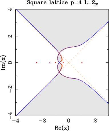
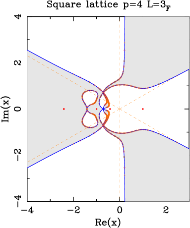
(((a)(a)	(((a)(b)
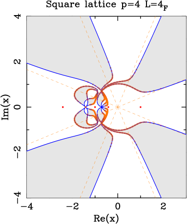
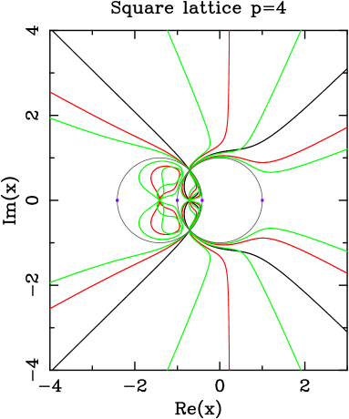
(((a)(c)	(((a)(d)

Figure 5: Limiting curves for the square-lattice RSOS model with $p=4$ and several widths: $L=2$ (a), $L=3$ (b), and $L=4$ (c). For each width $L$, we also show the partition-function zeros for finite strips of dimensions $L_{\text{F}}\times(10L)_{\text{P}}$ (black $\square$), $L_{\text{F}}\times(20L)_{\text{P}}$ (red $\circ$), and $L_{\text{F}}\times(30L)_{\text{P}}$ (brown $\triangle$). Figure (d) shows all these limiting curves together: $L=2$ (black), $L=3$ (red), $L=4$ (green). The solid squares $\blacksquare$ show the values where Baxter found the free energy. The symbol $\times$ in (a) marks the position of the found isolated limiting point. In the regions displayed in gray (resp.  white) the dominant eigenvalue comes from the sector $\chi_{1,3}$ (resp. $\chi_{1,1}$). The dark gray circles correspond to (1.5)

We have computed the limiting curves $\mathcal{B}_{L}$ for $L=2,3,4$. These curves are displayed in Figure 5(a)–(c). In Figure 5(d), we show simultaneously all three curves for comparison. In addition, we have computed the partition-function zeros for finite strips of dimensions $L_{\text{F}}\times(\rho L)_{\text{P}}$ for aspect rations $\rho=10,20,30$. These zeros are also displayed in Figure 5(a)–(c). For $5\leq L\leq 8$, we have only computed selected features of the corresponding limiting curves (e.g., the phase diagram for real $x$).

3.1.1 $\bm{L=2}$

This strip is displayed in Figure 3. Let us denote the basis in the height space as $|h_{1},h_{2},h_{3},h_{4},h_{5}\rangle$, where the order is given as in Figure 3.

The transfer matrix ${\mathsf{T}}_{1}$ is two-dimensional: in the basis $\{|1,2,1,2,1\rangle,|1,2,3,2,1\rangle\}$, it takes the form

$${\mathsf{T}}_{1}(p=4,L=2)\;=\;\frac{1}{\sqrt{2}}\,\left(\begin{array}[]{cc}Y_{2,0}&Y_{2,1}\\ Y_{2,3}&Y_{2,2}\end{array}\right)$$ (3.3)

where we have used the shorthand notation

$$Y_{L,k}\;=\;x^{k}\,\left(x+\sqrt{2}\right)^{2L-1-k}\,,\qquad k=0,\ldots,2L-1$$ (3.4)

The transfer matrix ${\mathsf{T}}_{3}$ is also two-dimensional: in the basis $\{|1,2,1,2,3\rangle,|1,2,3,2,3\rangle\}$, it takes the form

$${\mathsf{T}}_{3}(p=4,L=2)\;=\;\frac{1}{\sqrt{2}}\,\left(\begin{array}[]{cc}Y_{2,1}&Y_{2,2}\\ Y_{2,2}&Y_{2,1}\end{array}\right)$$ (3.5)

For real $x$, there is a single phase-transition point at

$$x_{\rm c}\;=\;-\frac{1}{\sqrt{2}}\approx-0.7071067812$$ (3.6)

This point is actually a multiple point. There is an additional pair of complex conjugate multiple points at $x=-e^{\pm i\pi/4}=-1/\sqrt{2}\pm i/\sqrt{2}$. We also find an isolated limiting point at $x=-\sqrt{2}$ due to the vanishing of all the eigenvalues (see Ref. [31] for an explanation of this issue in terms of the Beraha–Kahane–Weiss theorem).

The dominant sector on the real $x$-axis is always $\chi_{1,1}$, except at $x=-\sqrt{2}$ and $x=-1/\sqrt{2}$; at these points the dominant eigenvalues coming from each sector $\chi_{1,k}$ become equimodular. On the regions with null intersection with the real $x$-axis, the dominant eigenvalue comes from the sector $\chi_{1,3}$.

3.1.2 $\bm{L\geq 3}$

For $3\leq L\leq 8$, we find two phase-transition points on the real $x$-axis:

$$x_{{\rm c},1}&=-\frac{1}{\sqrt{2}}\approx-0.7071067812\\ x_{{\rm c},2}=-\sqrt{2}\approx-1.4142135624$$ (3.7)

Both points are actually multiple points (except $x_{{\rm c},2}$ for $L=3$). There is an additional pair of complex conjugate multiple points at $x=-e^{\pm i\pi/4}$.

For $x>x_{{\rm c},1}$, the dominant eigenvalue always belongs to the sector $\chi_{1,1}$. For $x<x_{{\rm c},1}$, this property is true only for even $L=4,6,8$; for odd $L=3,5,7$, the dominant eigenvalue for $x<x_{{\rm c},1}$ belongs to the $\chi_{1,3}$ sector.

3.2 $\bm{Q=B_{5}}$ model ($\bm{p=5}$)

The partition function for a strip of size $L_{\text{F}}\times N_{\text{P}}$ is given in the RSOS representation as

$$Z_{L_{\text{F}}\times N_{\text{P}}}(Q=B_{5};x)\;=\;B_{5}^{NL/2}\,\left[\chi_{1,1}(x)+\sqrt{B_{5}}\,\chi_{1,3}(x)\right]$$ (3.8)

where $\chi_{1,2j+1}(x)=\mathop{\rm tr}\nolimits{\mathsf{T}}_{2j+1}(p=5,L;x)^{N}$.

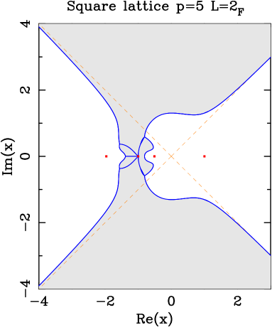
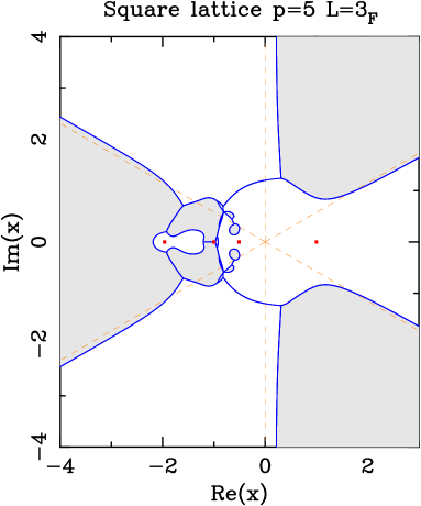
(((a)(a)	(((a)(b)
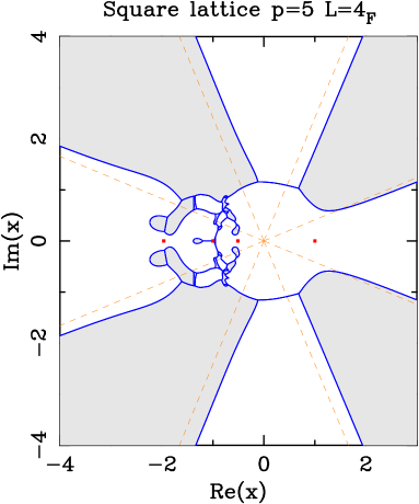
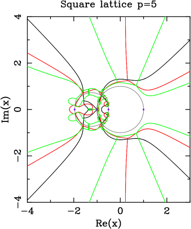
(((a)(c)	(((a)(d)

Figure 6: Limiting curves for the square-lattice RSOS model with $p=5$ and several widths: $L=2$ (a), $L=3$ (b), and $L=4$ (c). Figure (d) shows all these curves together: $L=2$ (black), $L=3$ (red), $L=4$ (green). The solid squares $\blacksquare$ show the values where Baxter found the free energy. In the regions displayed in light gray (resp.  white) the dominant eigenvalue comes from the sector $\chi_{1,3}$ (resp. $\chi_{1,1}$). The dark gray circles correspond to (1.5)

We have computed the limiting curves $\mathcal{B}_{L}$ for $L=2,3,4$. These curves are displayed in Figure 6(a)–(c). In Figure 6(d), we show all three curves for comparison. For $L=5,6$, we have only computed selected features of the corresponding limiting curves.

3.2.1 $\bm{L=2}$

The transfer matrix ${\mathsf{T}}_{1}$ is two-dimensional: in the basis $\{|1,2,1,2,1\rangle,|1,2,3,2,1\rangle\}$, it takes the form

$${\mathsf{T}}_{1}(p=5,L=2)\;=\;\left(\begin{array}[]{cc}\sqrt{B_{5}^{*}}X_{3}&B_{5}^{1/4}\sqrt{B_{5}^{*}}\,xX_{3}^{2}\\ B_{5}^{*\,1/4}\,x^{3}&x^{2}(1+x)\end{array}\right)$$ (3.9)

where we have used the shorthand notation

$$X_{3}\;=\;x+\sqrt{B_{5}}\,,\quad X_{3}^{*}\;=\;x+\sqrt{B_{5}^{*}}$$ (3.10)

in terms of $B_{5}$ and $B_{5}^{*}$ defined as

$$B_{5}\;=\;\frac{3+\sqrt{5}}{2}\,,\qquad B_{5}^{*}\;=\;\frac{3-\sqrt{5}}{2}$$ (3.11)

The transfer matrix ${\mathsf{T}}_{3}$ is three-dimensional. In the basis $\{|1,2,1,2,3\rangle,|1,2,3,4,3\rangle$, $|1,2,3,2,3\rangle\}$, it takes the form

$${\mathsf{T}}_{3}(p=5,L=2)\;=\;\left(\begin{array}[]{ccc}\sqrt{B_{5}^{*}}\,xX_{3}^{2}&0&B_{5}^{*\,1/4}\,x^{2}X_{3}\\ \sqrt{B_{5}^{*}}\,x^{2}&xX_{3}^{*}&B_{5}^{*\,1/4}\,x(1+x)\\ B_{5}^{*\,1/4}\,x^{2}(1+x)&B_{5}^{*\,1/4}\,x&x(1+x)^{2}\end{array}\right)$$ (3.12)

For real $x$, there is a single phase-transition point at

$$x_{\rm c}\;=\;-\frac{\sqrt{B_{5}}}{2}\;=\;-\frac{1+\sqrt{5}}{4}\;\approx\;-0.8090169944$$ (3.13)

We have also found that the limiting curve contains a horizontal line between $x=x_{\text{BK}}=-1$ and $x\approx-1.3843760945$. The latter point is a T point, and the former one, a multiple point. There is an additional pair of complex conjugate multiple points at

$$x\;=\;-e^{\pm i\pi/5}\;=\;-\frac{1+\sqrt{5}}{4}\pm\frac{i}{2}(5B_{5}^{*})^{1/4}\;\approx\;-0.8090169944\pm 0.5877852523\,i$$ (3.14)

We have found two additional pairs of complex conjugate T points at $x\approx-1.5613823329\pm 0.3695426938\,i$, and $x\approx-0.9270509831\pm 0.3749352940\,i$. The dominant sectors on the real $x$-axis are

• $\chi_{1,1}$ for $x\in(-\infty,-1.3843760945)\cup(-0.8090169944,\infty)$

• $\chi_{1,3}$ for $x\in(-1.3843760945,-0.8090169944)$

3.2.2 $\bm{L\geq 3}$

For $L=3$ there are two real phase-transition points at

$$x_{{\rm c},1}&\approx-2.1862990086\\ x_{{\rm c},2}\approx-0.9176152641$$ (3.15)

The limiting curve contains a horizontal line between two real T points $x\approx-1.2066212246$ and $x\approx-0.9713270390$. There are nine additional pairs of complex conjugate T points. The dominant sectors on the real $x$-axis are

• $\chi_{1,1}$ for $x\in(-2.1862990086,-1.2066212246)\cup(-0.9176152641,\infty)$

• $\chi_{1,3}$ for $x\in(-\infty,-2.1862990086)\cup(-1.2066212246,-0.9176152641)$

For $L=4$, the real transition points are located at

$$x_{{\rm c},1}&\approx-1.3829734471\\ x_{{\rm c},2}\approx-0.9475070976$$ (3.16)

We have found that the curve $\mathcal{B}_{4}$ contains a horizontal line between two real T points: $x\approx-1.1982787848$ and $x\approx-0.9776507663$. Two points belonging to such line are actually multiple points: $x\approx-0.9923357481$ and $x\approx-0.9972135728$. We have found 34 pairs of complex conjugate T points. The phase diagram is rather involved, and we find several tiny closed regions. The dominant sectors on the real $x$-axis are

• $\chi_{1,1}$ for $x\in(-\infty,x_{{\rm c},1})\cup(-1.1982787848,-0.9972135728)\cup(x_{{\rm c},2},\infty)$

• $\chi_{1,3}$ for $x\in(x_{{\rm c},1},-1.1982787848)\cup(-0.9972135728,x_{{\rm c},2})$

For $L=5$, there are four real phase-transition points at

$$x_{{\rm c},1}&\approx-2.4492425881\\ x_{{\rm c},2}\approx-1.2097913730\\ x_{{\rm c},3}\approx-1.1717714277\\ x_{{\rm c},4}\approx-0.9616402644$$ (3.17)

Again, $\mathcal{B}_{5}$ contains a horizontal line between $x\approx-1.1323655119$ and $x\approx-0.9770339631$. The dominant sectors on the real $x$-axis are

• $\chi_{1,1}$ for $x\in(x_{{\rm c},1},-0.9770339631)\cup(x_{{\rm c},4},\infty)$

• $\chi_{1,3}$ for $x\in(-\infty,x_{{\rm c},1})\cup(-0.9770339631,x_{{\rm c},4})$

Finally, for $L=6$, there are five real phase-transition points at

$$x_{{\rm c},1}&\approx-1.2750054535\\ x_{{\rm c},2}\approx-1.2712112920\\ x_{{\rm c},3}\approx-1.1323753929\\ x_{{\rm c},4}\approx-1.1052066740\\ x_{{\rm c},5}\approx-0.9700021428$$ (3.18)

The limiting curve contains a horizontal line between two real T points: $x\approx-1.0877465961$ and $x\approx-0.9792223546$. This line contains the multiple point $x\approx-1.0781213888$. The dominant sectors on the real $x$-axis are

• $\chi_{1,1}$ for $x\in(-\infty,x_{{\rm c},1})\cup(x_{{\rm c},2},-1.0877465961)\cup(-1.0781213888,\infty)$

• $\chi_{1,3}$ for $x\in(x_{{\rm c},1},x_{{\rm c},2})\cup(-1.0877465961,-1.0781213888)$

In all cases $2\leq L\leq 6$, there is a pair of complex conjugate multiple points at $x\;=\;-e^{\pm i\pi/5}\approx-0.8090169944\pm 0.5877852523\,i$.

3.3 Three-state Potts model ($\bm{p=6}$)

The partition function for a strip of size $L_{\text{F}}\times N_{\text{P}}$ is given in the RSOS representation as

$$Z_{L_{\text{F}}\times N_{\text{P}}}(Q=3;x)\;=\;3^{NL/2}\left[\chi_{1,1}(x)+2\chi_{1,3}(x)+\chi_{1,5}(x)\right]$$ (3.19)

where $\chi_{1,2j+1}(x)=\mathop{\rm tr}\nolimits{\mathsf{T}}_{2j+1}(p=6,L;x)^{N}$.

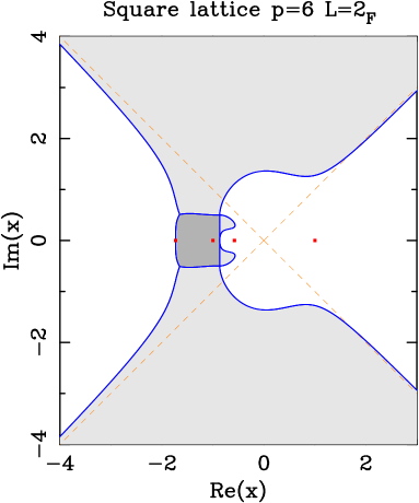
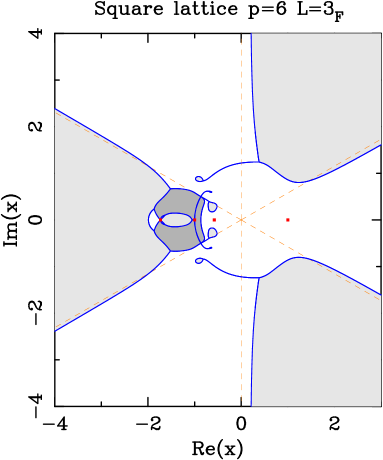
(((a)(a)	(((a)(b)
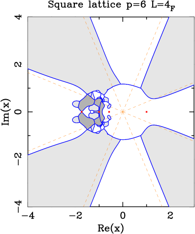
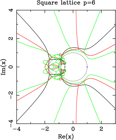
(((a)(c)	(((a)(d)

Figure 7: Limiting curves for the square-lattice RSOS model with $p=6$ and several widths: $L=2$ (a), $L=3$ (b), and $L=4$ (c). Figure (d) shows all these curves together: $L=2$ (black), $L=3$ (red), $L=4$ (green). The solid squares $\blacksquare$ show the values where Baxter found the free energy. In the regions displayed in light gray (resp.  white) the dominant eigenvalue comes from the sector $\chi_{1,3}$ (resp. $\chi_{1,1}$). In the regions displayed in a darker gray the dominant eigenvalue comes from the sector $\chi_{1,5}$. The dark gray circles correspond to (1.5)

We have computed the limiting curves $\mathcal{B}_{L}$ for $L=2,3,4$. These curves are displayed in Figure 7(a)–(c).

In Figure 7(d), we show all three curves for comparison. For $L=5,6,7$ we have only computed selected features of the corresponding limiting curves.

3.3.1 $\bm{L=2}$

The transfer matrix ${\mathsf{T}}_{5}$ is one-dimensional, as there is a single basis vector $\{|1,2,3,4,5\rangle\}$. The matrix is given by

$${\mathsf{T}}_{5}(p=6,L=2)=x^{2}$$ (3.20)

The transfer matrix ${\mathsf{T}}_{1}$ is two-dimensional: in the basis $\{|1,2,1,2,1\rangle,|1,2,3,2,1\rangle\}$, it takes the form

$${\mathsf{T}}_{1}(p=6,L=2)\;=\;\frac{1}{\sqrt{3}}\,\left(\begin{array}[]{cc}X_{1}^{3}&\sqrt{2}\,x\,X_{1}^{2}\\ \sqrt{2}\,x^{3}&x^{2}X_{2}\end{array}\right)$$ (3.21)

where we have used the shorthand notation

$$X_{1}\;=\;x+\sqrt{3}\,,\quad X_{2}\;=\;2x+\sqrt{3}$$ (3.22)

The transfer matrix ${\mathsf{T}}_{3}$ is three-dimensional. In the basis $\{|1,2,1,2,3\rangle,|1,2,3,4,3\rangle$, $|1,2,3,2,3\rangle\}$, it takes the form

$${\mathsf{T}}_{3}(p=6,L=2)\;=\;\frac{1}{2\sqrt{3}}\,\left(\begin{array}[]{ccc}2\,xX_{1}^{2}&0&2\sqrt{2}\,x^{2}X_{1}\\ \sqrt{6}\,x^{2}&\sqrt{3}\,xX_{2}&\sqrt{3}\,xX_{2}\\ \sqrt{2}\,x^{2}X_{2}&3\,x&xX_{2}^{2}\end{array}\right)$$ (3.23)

For real $x$, there are two phase-transition points

$$x_{{\rm c},1}&=-\sqrt{3}\;=\;x_{-}\;\approx\;-1.7320508076\\ x_{{\rm c},2}=-\frac{\sqrt{3}}{2}\;\approx\;-0.8660254038$$ (3.24)

There is one pair of complex conjugate T points at $x\approx-1.6522167507\pm 0.5104474197\,i$. There are three multiple points at $x=-\sqrt{3}/2$, and $x=-\sqrt{3}/2\pm i/2=-e^{\pm i\pi/6}$. The dominant sectors on the real $x$-axis are

• $\chi_{1,1}$ for $x\in(-\infty,-\sqrt{3})\cup(-\sqrt{3}/2,\infty)$

• $\chi_{1,5}$ for $x\in(-\sqrt{3},-\sqrt{3}/2)$

On the regions with null intersection with the real $x$-axis, the dominant eigenvalue comes from the sector $\chi_{1,3}$.

3.3.2 $\bm{L\geq 3}$

For $L=3$, there are three real phase-transition points

$$x_{{\rm c},1}&\approx-1.9904900679\\ x_{{\rm c},2}=-\sqrt{3}\;=\;x_{-}\;\approx\;-1.7320508076\\ x_{{\rm c},3}=-\frac{\sqrt{3}}{2}\;\approx\;-0.8660254038$$ (3.25)

The limiting curve contains a small horizontal segment running from $x\approx-1.0539518478$ to $x=x_{\text{BK}}=-1$. On this line, the two dominant equimodular eigenvalues come from the sector $\chi_{1,5}$.

We have found 15 T points (one real point and seven pairs of complex conjugate T points). The real point is $x=-1$. The phase structure is vastly more complicated than that for $L=2$. In particular, it contains three non-connected pieces, and four bulb-like regions. On the real $x$-axis, the dominant eigenvalue comes from

• $\chi_{1,1}$ for $x\in(x_{{\rm c},1},-\sqrt{3})\cup(-\sqrt{3}/2,\infty)$

• $\chi_{1,3}$ for $x\in(-\infty,x_{{\rm c},1})\cup(-\sqrt{3},-1.0539518478)$

• $\chi_{1,5}$ for $x\in(-1.0539518478,-\sqrt{3}/2)$

For $L=4$, there are four phase-transition points

$$x_{{\rm c},1}&=-\sqrt{3}\;=\;x_{-}\;\approx\;-1.7320508076\\ x_{{\rm c},2}\approx-1.3678583305\\ x_{{\rm c},3}\approx-1.2237725061\\ x_{{\rm c},4}=-\frac{\sqrt{3}}{2}\;\approx\;-0.8660254038$$ (3.26)

This is the strip with smallest width for which a (complex conjugate) pair of endpoints appears: $x\approx-0.9951436066\pm 0.00444309186\,i$. These points are very close to the transition point $x_{\text{BK}}=-1$. We have found 36 pairs of conjugate T points. We have also found three multiple points at $x=-\sqrt{3}$, and $x=-\sqrt{3}/2\pm i/2$. The dominant sectors on the real $x$-axis are

• $\chi_{1,1}$ for $x\in(-\infty,x_{{\rm c},3})\cup(-\sqrt{3}/2,\infty)$

• $\chi_{1,5}$ for $x\in(x_{{\rm c},3},-\sqrt{3}/2)$

For $L=5$, there are six real phase-transition points

$$x_{{\rm c},1}&\approx-2.3018586529\\ x_{{\rm c},2}=-\sqrt{3}\;=\;x_{-}\;\approx\;-1.7320508076\\ x_{{\rm c},3}\approx-1.4373407728\\ x_{{\rm c},4}\approx-1.3412360954\\ x_{{\rm c},5}\approx-1.2613579653\\ x_{{\rm c},6}=-\frac{\sqrt{3}}{2}\;\approx\;-0.8660254038$$ (3.27)

We have also found a horizontal line running between the T points $x\approx-1.0226306002$ and $x\approx-0.9984031794$. The dominant sectors on the real $x$-axis are

• $\chi_{1,1}$ for $x\in(x_{{\rm c},1},x_{{\rm c},3})\cup(-\sqrt{3}/2,\infty)$

• $\chi_{1,3}$ for $x\in(-\infty,x_{{\rm c},1})\cup(x_{{\rm c},3},-1.0226306002)$

• $\chi_{1,5}$ for $x\in(-1.0226306002,-\sqrt{3}/2)$

For $L=6$, there are also six phase-transition points on the real axis

$$x_{{\rm c},1}&=-\sqrt{3}\;=\;x_{-}\;\approx\;-1.7320508076\\ x_{{\rm c},2}\approx-1.2852299467\\ x_{{\rm c},3}\approx-1.2238569234\\ x_{{\rm c},4}\approx-1.1271443188\\ x_{{\rm c},5}\approx-1.0085262838\\ x_{{\rm c},6}=-\frac{\sqrt{3}}{2}\;\approx\;-0.8660254038$$ (3.28)

The dominant sectors on the real $x$-axis are

• $\chi_{1,1}$ for $x\in(-\infty,x_{{\rm c},2})\cup(x_{{\rm c},3},x_{{\rm c},5})\cup(-\sqrt{3}/2,\infty)$

• $\chi_{1,5}$ for $x\in(x_{{\rm c},2},x_{{\rm c},3})\cup(x_{{\rm c},5},-\sqrt{3}/2)$

In all cases $2\leq L\leq 6$, we have found three multiple points at $x=-\sqrt{3}$, and $x=-\sqrt{3}/2\pm i/2=-e^{\pm i\pi/6}$.

3.4 Four-state Potts model ($p=\infty$)

It follows from the RSOS constraint and the fact that $h_{0}=1$ is fixed, that the maximal height participating in a state is $h_{\rm max}=\text{max}(2L,p-1)$. In particular, for any fixed $L$ the number of states stays finite when one takes the limit $p\to\infty$. Meanwhile, the Boltzmann weight entering in Eq. (2.7) has the well-defined limit $(h_{j}h^{\prime}_{j})^{1/2}/h_{j-1}$, and the amplitudes (2.2) tend to $S_{j}(\infty)=2j+1$. We shall refer to this limit as the $p=\infty$ (or $Q=4$) model.

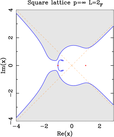
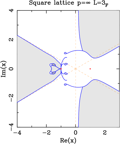
(((a)(a)	(((a)(b)
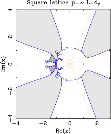
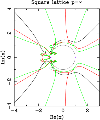
(((a)(c)	(((a)(d)

Figure 8: Limiting curves for the square-lattice RSOS model with $p=\infty$ ($Q=4$) and several widths: $L=2$ (a), $L=3$ (b), and $L=4$ (c). Figure (d) shows all these curves together: $L=2$ (black), $L=3$ (red), $L=4$ (green). The solid squares $\blacksquare$ show the values where Baxter found the free energy. In the regions displayed in light gray (resp.  white) the dominant eigenvalue comes from the sector $\chi_{1,3}$ (resp. $\chi_{1,1}$). In the regions displayed in a darker gray the dominant eigenvalue comes from the sector $\chi_{1,5}$.

We have computed the limiting curves $\mathcal{B}_{L}$ for $L=2,3,4$. These curves are displayed in Figure 8(a)–(c). In Figure 8(d), we show all three curves for comparison.

3.4.1 $\bm{L=2}$

The transfer matrices are

$${\mathsf{T}}_{1}&=\frac{1}{2}\,\left(\begin{array}[]{cc}(x+2)^{3}&\sqrt{3}\,x(x+2)^{2}\\ \sqrt{3}\,x^{3}&x^{2}(2+3x)\end{array}\right)\\ T_{3}=\frac{1}{6}\,\left(\begin{array}[]{ccc}3x(x+2)^{2}&0&3\sqrt{3}\,x^{2}(x+2)\\ 2\sqrt{6}\,x^{2}&2x(3x+4)&2\sqrt{2}\,x(3x+2)\\ \sqrt{3}\,x^{2}(3x+2)&4\sqrt{2}\,x&x(3x+2)^{2}\end{array}\right)\\ T_{5}=x^{2}$$ (3.29)

For real $x$, we find a multiple point at $x=-1$, where all eigenvalues become equimodular with $|\lambda_{i}|=1$. The dominant sector on the real $x$-axis is always $\chi_{1,1}$.

3.4.2 $\bm{L\geq 3}$

For $L=3$ there are two real phase-transition points: $x=-1$ (which is a multiple point), and $x_{c}\approx-1.6424647621$. We have found ten pairs of complex conjugate T points and a pair of complex conjugate endpoints. The dominant sectors on the real $x$-axis are $\chi_{1,3}$ for $x<-1$, and $\chi_{1,1}$ for $x>-1$. The sector $\chi_{1,5}$ is only dominant in two complex conjugate regions off the real $x$-axis, and the sector $\chi_{1,7}$ is never dominant.

For $L=4$ we only find a single real phase-transition point at $x=-1$. We have also found 32 pairs of complex conjugate T points and two pairs of complex conjugate endpoints. The dominant sector on the real $x$-axis is always $\chi_{1,1}$. There is also two complex conjugate regions where the dominant eigenvalue comes from the sector $\chi_{1,5}$, and the sectors $\chi_{1,7}$ and $\chi_{1,9}$ are never dominant in the complex $x$-plane.

For $L=5$ we find four real phase-transition points at

$$x_{c,1}&=-1.9465787472\\ x_{c,2}=-1.5202407889\\ x_{c,3}=-1.3257163278\\ x_{c,4}=-1$$ (3.30)

The dominant sectors are $\chi_{1,3}$ for $x\in(-\infty,x_{c,1})\cup(x_{c,2},-1)$; and $\chi_{1,1}$ in the region $x\in(x_{c,1},x_{c,2})\cup(-1,\infty)$.

For $L=4$ we only find a single real phase-transition point at $x=-1$. The dominant sector on the real $x$-axis is always $\chi_{1,1}$.

In all cases $3\leq L\leq 5$, the point $x=-1$ is a multiple point where all the eigenvalues are equimodular with $|\lambda_{i}|=1$.

4 Common features of the square-lattice limiting curves with free cyclic boundary conditions

From the numerical data discussed in Sections 3.1–3.3, we can make the following conjecture that states that certain points in the complex $x$-plane belong to the limiting curve $\mathcal{B}_{L}$:

Conjecture 4.1

For the square-lattice $Q$-state Potts model with $Q=B_{p}$ and widths $L\geq 2$:

1. The points $x=-e^{\pm i\pi/p}$ belong to the limiting curve. At these points, all the eigenvalues are equimodular with $|\lambda_{i}|=1$. Thus, they are in general multiple points.

2. For even $p$, the point $x=-\sqrt{Q}/2$ always belongs to the limiting curve $\mathcal{B}_{L}$. Furthermore, if $p=4,6$, then the point $x=-\sqrt{Q}$ also belongs to $\mathcal{B}_{L}$.

The phase structure for the models considered above show certain regularities on the real $x$-axis (which contains the physical regime of the model). In particular, we conclude

Conjecture 4.2

For the square-lattice $Q$-state Potts model with $Q=B_{p}$ and widths $L\geq 2$:

1. The relevant eigenvalue on the physical line $v\in[-1,\infty)$ comes from the sector $\chi_{1,1}$.

2. For even $L$, the leading eigenvalue for real $x$ comes always from the sector $\chi_{1,1}$, except perhaps in an interval contained in $[-\sqrt{Q},-\sqrt{Q}/2]$.

3. For odd $L$, the leading eigenvalue for real $x$ comes from the sector $\chi_{1,3}$ for all $x<x_{0}\leq-\sqrt{Q}$, and from the sector $\chi_{1,1}$ for all $x\geq-\sqrt{Q}/2$.

In the limiting case $p=\infty$ the RSOS construction simplifies. Namely, the quantum group $U_{q}(SU(2))$ reduces to the classical $U(SU(2))$ (i.e., $q\to 1$), and its representations no longer couple different $K_{1,2j+1}$, cf. Eq. (2.4). Accordingly we have simply $K_{1,2j+1}=\chi_{1,2j+1}$. When increasing $p$ along the line $x_{\rm BK}(Q)$, the sector $K_{1,2j+1}$ which dominates for irrational $p$ will have higher and higher spin $j$ [7]; this is even true throughout the Berker-Kadanoff phase. One would therefore expect that the $p=\infty$ RSOS model will have a dominant sector $\chi_{1,2j+1}$ with $j$ becoming larger and larger as one approaches $x_{BK}(Q=4)=-1$.

This argument should however be handled with care. Indeed, for $p\to\infty$ the BK phase contracts to a point, $(Q,v)=(4,-2)$, and this point turns out to be a very singular limit of the Potts model. In particular, one has $x_{\rm BK}=x_{\pm}$ for $Q=4$, and very different results indeed are obtained depending on whether one approaches $(Q,v)=(4,-2)$ along the AF or the BK curves (1.4). This is visible, for instance, on the level of the central charge, with $c\to 2$ in the former and $c\to-\infty$ in the latter case. To wit, taking $x\to-1$ after having fixed $p=\infty$ in the RSOS model is yet another limiting prescription, which may lead to different results.

The phase diagrams for $Q=4$ ($p\to\infty$) do agree with the above general conjectures 4.1-4.2. In particular, when $p\to\infty$, the multiple points $-e^{\pm i\pi/p}\to-1=x_{\text{BK}}$ (Conjecture 4.1.1) and this coincides with the point $-\sqrt{Q}/2$ (Conjecture 4.1.2). On the other hand, the sector $\chi_{1,1}$ is the dominant one on the physical line $v\in[-1,\infty)$ (Conjecture 4.2.1), and we observe a parity effect on the unphysical regime $v\in(-\infty,-1)$. For even $L$, the only dominant sector is $\chi_{1,1}$ in agreement with Conjecture 4.2.2 (although there is no interval inside $[-2,-1]$ where $\chi_{1,3}$ becomes dominant). For odd $L$, Conjecture 4.2.3 also holds with $x_{0}=-\sqrt{Q}=-2$ (at least for $L=3,5$). For $L=2,3,4$, we find that in addition to the sectors $\chi_{1,1}$ and $\chi_{1,3}$, only the sector $\chi_{1,5}$ becomes relevant in some regions in the complex $x$-plane.

4.1 Asymptotic behavior for $\bm{|x|\to\infty}$

Figures 5–8 show a rather uncommon scenario: the limiting curves contain outward branches. As a matter of fact, these branches extend to infinity (i.e., they are unbounded), in sharp contrast with the bounded limiting curves obtained using free longitudinal boundary conditions [39, 40]. It is important to remark that this phenomenon also holds in the limit $p\to\infty$, as shown in Figure 8.

As $|x|\to\infty$ these branches converge to rays with definite slopes. More precisely, our numerical data suggest the following conjecture:

Conjecture 4.3

For any value of $p$, the limiting curve $\mathcal{B}_{L}$ for a square-lattice strip has exactly $2L$ outward branches. As $|x|\to\infty$, these branches are asymptotically rays with

$$\arg x\;\equiv\;\theta_{n}(L)\;=\;\pi\left(\frac{n}{L}-\frac{1}{2L}\right)\,,\qquad n=1,2,\ldots,2L$$ (4.1)

By inspection of Figures 5–8, it is also clear that the only two sectors that are relevant in this regime are $\chi_{1,1}$ and $\chi_{1,3}$. In particular, the dominant eigenvalue belongs to the $\chi_{1,1}$ sector for large positive real $x$, and each time we cross one of these outward branches, the dominant eigenvalue switches the sector it comes from. In particular, we conjecture that

Conjecture 4.4

The dominant eigenvalue for a square-lattice strip of width $L$ in the large $|x|$ regime comes from the sector $\chi_{1,1}$ in the asymptotic regions

$$\arg x\;\in\;\left(\theta_{2n-1}(L),\theta_{2n}(L)\right)\,,\qquad n=1,2,\ldots,L$$ (4.2)

In the other asymptotic regions the dominant eigenvalue comes from the sector $\chi_{1,3}$.

In particular, this means that for large positive $x$ the dominant sector is always $\chi_{1,1}$. However, for large negative $x$ the dominant eigenvalue comes from $\chi_{1,1}$ is $L$ is even, and from $\chi_{1,3}$ if $L$ is odd. Thus, this conjecture is compatible with Conjecture 4.2.

An empirical explanation of this fact comes from the computation of the asymptotic expansion for large $|x|$ of the leading eigenvalues in each sector. It turns out that there is a unique leading eigenvalue in each sector $\chi_{1,1}$ and $\chi_{1,3}$ when $|x|\to\infty$. As there is a unique eigenvalue in this regime, we can obtain it by the power method [44]. Our numerical results suggest the following conjecture

Conjecture 4.5

Let $\lambda_{\star,1}(L)$ (resp. $\lambda_{\star,3}$(L)) be the leading eigenvalue of the sector $\chi_{1,1}$ (resp.  $\chi_{1,3}$) in the regime $|x|\to\infty$. Then

$$\lambda_{\star,1}(L)&=Q^{(L-1)/2}\,x^{2L-1}\,\left[1+\sum\limits_{k=1}^{\infty}\frac{a_{k}(L)}{Q^{k/2}}\,x^{-k}\right]\\ \lambda_{\star,1}(L)-\lambda_{\star,3}(L)=\sqrt{Q}\,x^{L-1}+3(L-1)x^{L-2}+O(x^{L-3})$$ (4.3)

Furthermore, we have that

$$a_{1}(L)&=2L-1\,,\qquad L\geq 2\\ a_{2}(L)=2L^{2}-3L+1\,,\qquad L\geq 3$$ (4.4)

The first coefficients $a_{k}(L)$ are displayed in Table 1; the patterns displayed in (4.4) are easily verified. The coefficients $a_{k}(L)$ also depend on $p$ for $k\geq 3$.

Indeed, the above conjecture explains easily the observed pattern for the leading sector when $x$ is real. But it also explains the observed pattern for all the outward branches. These branches are defined by the equimodularity of the two leading eigenvalues

$$|\lambda_{\star,1}|\;=\;|\lambda_{\star,3}|\;=\;\left|\lambda_{\star,1}-\sqrt{Q}x^{L-1}+O(x^{L-2})\right|$$ (4.5)

This implies that

$$\mathop{\rm Re}\nolimits\left[\lambda_{\star,1}\,\overline{x}^{L-1}\right]\;=\;0$$ (4.6)

where $\overline{x}$ is the complex conjugate of $x$. Then, if $x=|x|e^{i\theta}$, then the above equation reduces to

$$\cos\left(\theta L\right)\;=\;0\;\Rightarrow\;\theta_{n}=\frac{\pi}{2L}(2n-1)\,,\quad n=1,2,\dots,2L$$ (4.7)

in agreement with Eq. (4.1).

Remark. The existence of unbounded outward branches for the limiting curve of the Potts model with cyclic boundary conditions is already present for the simplest case $L=1$. Here, the strip is just the cyclic graph of $n$ vertices $C_{n}$. Its partition function is given exactly by

$$Z_{C_{n}}(Q,v)\;=\;(Q+v)^{n}+(Q-1)\,v^{n}$$ (4.8)

Then, we have two eigenvalues $\lambda_{1}=Q+v=Q+x\sqrt{Q}$ and $\lambda_{2}=v=x\sqrt{Q}$, which grow like $\sim x^{2L-1}=x$ and whose difference is $Q=O(x^{L-1})$, in agreement with Conjecture 4.5. Furthermore, the limiting curve is the line $\mathop{\rm Re}\nolimits x=-\sqrt{Q}/2$, which, as $|x|\to\infty$, has slopes given by $\pm\pi/2$, in agreement with Conjecture 4.3.

4.2 Other asymptotic behaviors

For the Ising case ($p=4$) the points $x=-\sqrt{2}$ and $x=-1/\sqrt{2}$ are in general multiple points and we observe a pattern similar to the one observed for $|x|\to\infty$.

For $x=-1/\sqrt{2}$, we find that, if we write $x=-1/\sqrt{2}+\epsilon$ with $|\epsilon|\ll 1$, within each sector there is only one leading eigenvalue $\lambda_{\star,j}(L)\sim O(1)$. More precisely, for $L\geq 3$,

$$\lambda_{\star,1}(L)&=2^{-L/2}+O(\epsilon^{3})\\ \lambda_{\star,1}(L)-\lambda_{\star,3}(L)=2\epsilon^{L}+O(\epsilon^{L+1})$$ (4.9)

Again, the equimodularity condition when $|\epsilon|\to 0$ implies that $\mathop{\rm Re}\nolimits(\epsilon^{L})=0$, whence $\arg\epsilon=\theta_{n}$ with $\theta_{n}$ given by Eq. (4.7).

The case $x=-\sqrt{2}$ is more involved. If we write $x=-\sqrt{2}+\epsilon$ with $|\epsilon|\ll 1$, we find that in the sector $\chi_{1,1}$ there are two eigenvalues of order $O(\epsilon)$, and the rest are of order at least $O(\epsilon^{2})$. The same conclusion is obtained from the sector $\chi_{1,3}$. If we call $\lambda_{\star,j}^{(i)}$ ($i=1,2$) the dominant eigenvalues coming from sector $\chi_{1,j}$, then we find for $L\geq 3$ that

$$\lambda_{\star,1}^{(1)}(L)&=2^{(L-1)/2}\epsilon+O(\epsilon^{2})\;\approx\;-\lambda_{\star,1}^{(2)}(L)\\ \lambda_{\star,1}^{(1)}(L)+\lambda_{\star,1}^{(2)}(L)=\begin{cases}\sqrt{2}\epsilon^{L-1}&\quad\text{$L$ even}\\ 2(L-1)\epsilon^{L}&\quad\text{$L$ odd}\end{cases}\\ \lambda_{\star,3}^{(1)}(L)=-2^{(L-1)/2}\epsilon+O(\epsilon^{2})\;\approx\;-\lambda_{\star,3}^{(2)}(L)\\ \lambda_{\star,3}^{(1)}(L)+\lambda_{\star,3}^{(2)}(L)=\begin{cases}-2(L-1)\epsilon^{L}&\quad\text{$L$ even}\\ -\sqrt{2}\epsilon^{L-1}&\quad\text{$L$ odd}\end{cases}\\ \lambda_{\star,1}^{(1)}(L)+\lambda_{\star,3}^{(1)}(L)=\frac{(-1)^{L}}{\sqrt{2}}\epsilon^{L-1}+O(\epsilon^{L})$$ (4.10)

The equimodularity condition implies that

$$\mathop{\rm Re}\nolimits\left[\epsilon\,\overline{\epsilon}^{L-1}\right]\;=\;0\;\Rightarrow\;\cos(\theta(L-2))\;=\;0$$ (4.11)

Thus, the same asymptotic behavior is obtained as for $x=-1/\sqrt{2}$, except that $L\to L-2$:

$$\theta_{n}\;=\;\frac{\pi}{2(L-2)}(2n-1)\,,\qquad n=1,\ldots,2(L-2)$$ (4.12)

5 Triangular-lattice Potts model with free cyclic boundary conditions

5.1 Ising model ($\bm{p=4}$)

For this model we know [16, 17, 18] the exact transition temperature for the antiferromagnetic model $v_{{\rm c},\text{AF}}=-1=v_{{\rm c},\text{BK}}$. The partition function is given by a formula similar to that of the square lattice, and the dimensionality of ${\mathsf{T}}_{j}(2,L)$ is the same as for the square lattice. In what follows we give the different matrices in the same bases as for the square lattice.

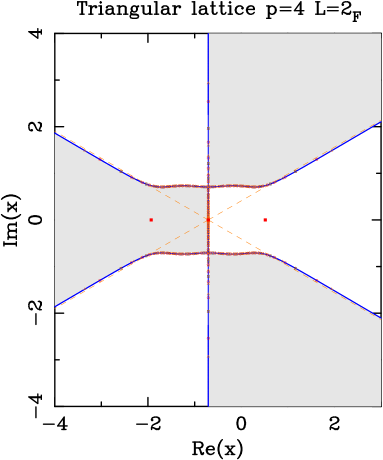
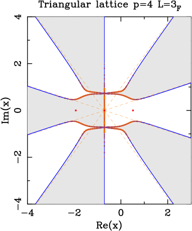
(((a)(a)	(((a)(b)
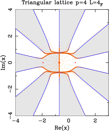
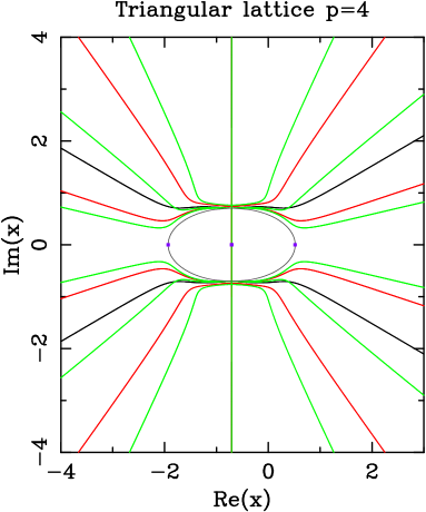
(((a)(c)	(((a)(d)

Figure 9: Limiting curves for the triangular-lattice RSOS model with $p=4$ and several widths: $L=2$ (a), $L=3$ (b), and $L=4$ (c). For each width $L$, we also show the partition-function zeros for finite strips of dimensions $L_{\text{F}}\times(10L)_{\text{P}}$ (black $\square$), $L_{\text{F}}\times(20L)_{\text{P}}$ (red $\circ$), and $L_{\text{F}}\times(30L)_{\text{P}}$ (brown $\triangle$). Figure (d) shows all these limiting curves together: $L=2$ (black), $L=3$ (red), $L=4$ (green). The solid squares $\blacksquare$ show the values where Baxter found the free energy. The symbol $\times$ in (a) marks the position of the found isolated limiting point. In the regions displayed in gray (resp.  white) the dominant eigenvalue comes from the sector $\chi_{1,3}$ (resp. $\chi_{1,1}$). The gray ellipse corresponds to $(\mathop{\rm Re}\nolimits x+1/\sqrt{2})^{2}+3(\mathop{\rm Im}\nolimits x)^{2}=3/2$. This curve goes through the points $x=-e^{\pm i\,\pi/4}$.

We have computed the limiting curves $\mathcal{B}_{L}$ for $L=2,3,4$. These curves are displayed in Figure 9(a)–(c). In Figure 9(d), we show all three curves for comparison.

5.1.1 $\bm{L=2}$

This strip is drawn in Figure 4. The transfer matrices are

$${\mathsf{T}}_{1}&=\frac{1}{2}\,\left(\begin{array}[]{cc}2x^{4}+5\sqrt{2}x^{3}+12x^{2}+8\sqrt{2}x+4&x(2x^{3}+5\sqrt{2}x^{2}+8x+2\sqrt{2})\\ x^{2}(2x^{2}+3\sqrt{2}x+2)&x^{2}(2x^{2}+3\sqrt{2}x+2)\end{array}\right){}\\ T_{3}=\frac{x}{2}\,\left(\begin{array}[]{cc}2x^{3}+5\sqrt{2}x^{2}+8x+2\sqrt{2}&2x^{3}+5\sqrt{2}x^{2}+8x+2\sqrt{2}\\ x(2x^{2}+3\sqrt{2}x+2)&8x^{3}+3\sqrt{2}x^{2}+6x+2\sqrt{2}\end{array}\right){}$$ (5.1)

For real $x$, there is a single phase-transition point at

$$x_{\rm c}\;=\;-1/\sqrt{2}\;\approx\;-0.7071067812$$ (5.2)

We have found that the entire line

$$\mathop{\rm Re}\nolimits x\;=\;-1/\sqrt{2}$$ (5.3)

belongs to the limiting curve. Furthermore, $\mathcal{B}_{2}$ is symmetric with respect to this line. Finally, there are two complex conjugate multiple points at $x=-1/\sqrt{2}\pm i/\sqrt{2}=-e^{\pm i\pi/4}$.

The dominant sector on the real $x$-axis is $\chi_{1,1}$ for $x>-1/\sqrt{2}$, and $\chi_{1,3}$ for $x<-1/\sqrt{2}$. Note that $x_{\rm c}=-1/\sqrt{2}$ gives the right bulk critical temperature for this model in the antiferromagnetic regime.

5.1.2 $\bm{L\geq 3}$

For $L=3,4$ we have found that a) The line $\mathop{\rm Re}\nolimits x=-1/\sqrt{2}$ belongs to the limiting curve; b) $\mathcal{B}_{L}$ is symmetric under reflection with respect to that line; c) $\mathcal{B}_{L}$ contains a pair of multiple points at $x=-e^{\pm i\pi/4}$; and d) The dominant sector on the real $x$-axis is $\chi_{1,1}$ for $x>-1/\sqrt{2}$, and $\chi_{1,3}$ for $x<-1/\sqrt{2}$.

For $L=3$, there is another pair of multiple points at $x\approx-1/\sqrt{2}\pm 0.7257238112\,i$; for $L=4$ this pair is located at $x\approx-1/\sqrt{2}\pm 0.7647261156\,i$.

For $L=5,6,7$, we have found that there is a single real phase-transition point at $x=-1/\sqrt{2}$, and that the dominant sector for $x>-1/\sqrt{2}$ (resp.  $x<-1/\sqrt{2}$) is $\chi_{1,1}$ (resp.  $\chi_{1,3}$).

5.2 $\bm{Q=B_{5}}$ model ($\bm{p=5}$)

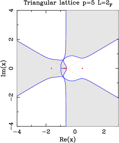
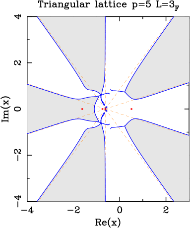
(((a)(a)	(((a)(b)
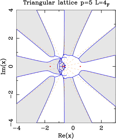
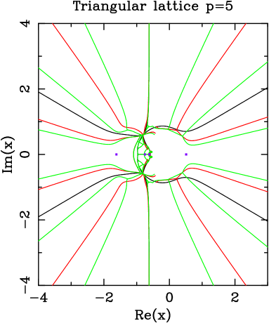
(((a)(c)	(((a)(d)

Figure 10: Limiting curves for the RSOS model with $p=5$ and several widths: $L=2$ (a), $L=3$ (b), and $L=4$ (c). Figure (d) shows all these curves together: $L=2$ (black), $L=3$ (red), $L=4$ (green). The solid squares $\blacksquare$ show the values where Baxter found the free energy. In the regions displayed in light gray (resp.  white) the dominant eigenvalue comes from the sector $\chi_{1,3}$ (resp. $\chi_{1,1}$).

We have computed the limiting curves $\mathcal{B}_{L}$ for $L=2,3,4$. These curves are displayed in Figure 10(a)–(c). In Figure 10(d), we show all three curves for comparison.

5.2.1 $\bm{L=2}$

The transfer matrices are

$${\mathsf{T}}_{1}&=\left(\begin{array}[]{cc}B_{5}+x(2x+4X_{3}+x^{2}X_{4}^{\star})&xB_{5}^{1/4}(\sqrt{B_{5}}+4x+x^{2}X_{5}^{\star})\\ x^{2}B_{5}^{1/4}(1+3\sqrt{B_{4}^{\star}}x+x^{2})&x^{2}(1+3x+3\sqrt{B_{5}}x^{2})\end{array}\right){}\\ {\mathsf{T}}_{3}=x\,\left(\begin{array}[]{ccc}\sqrt{B_{5}}+4x+x^{2}X_{4}^{\star}&\sqrt{B_{5}^{\star}}X_{3}&B_{5}^{1/4}(1+x\sqrt{5B_{5}}+x^{2}X_{4}^{\star})\\ \sqrt{B_{5}^{\star}}x&X_{3}^{\star}&(B_{5}^{\star})^{1/4}(1+x)\\ (B_{5}^{\star})^{1/4}x(1+3x+\sqrt{B_{5}}x^{2})&(B_{5}^{\star})^{1/4}(1+x)&1+3x+3x^{2}+\sqrt{B_{5}}x^{3}\end{array}\right)\\ {}$$ (5.4)

where we have defined the shorthand notations

$$X_{4}^{\star}&=1+3\sqrt{B_{5}^{\star}}+X_{3}^{\star}\\ X_{5}^{\star}=1+4\sqrt{B_{5}^{\star}}+X_{3}^{\star}$$ (5.5)

For real $x$, there are two phase-transition points at

$$x_{{\rm c},1}&\approx-0.9630466372\\ x_{{\rm c},2}\approx-0.5908569607$$ (5.6)

In fact both points are T points and the whole interval $[x_{{\rm c},1},x_{{\rm c},2}]$ belongs to the limiting curve $\mathcal{B}_{2}$. Finally, there are two complex conjugate multiple points at $x=-e^{\pm i\pi/5}$, as for the square-lattice case. The dominant sector on the real $x$-axis is $\chi_{1,1}$ for $x>x_{{\rm c},1}$, and $\chi_{1,3}$ for $x<x_{{\rm c},1}$.

5.2.2 $\bm{L\geq 3}$

For $L=3$, there are two real phase-transition points at

$$x_{{\rm c},1}&\approx-1.0976251052\\ x_{{\rm c},2}\approx-0.6376476917$$ (5.7)

We have found two pairs of complex conjugate endpoints at $x\approx-0.4297467004\pm 0.6445268125\,i$, and $x\approx-0.3955590901\pm 0.8536454650\,i$. There are nine pairs of complex conjugate T points, and two complex conjugate multiple points at $x=-e^{\pm i\pi/5}$. The dominant sectors on the real $x$-axis are $\chi_{1,1}$ for $x>x_{{\rm c},1}$, and $\chi_{1,3}$ for $x<x_{{\rm c},1}$

For $L=4$, there are three real phase-transition points at

$$x_{{\rm c},1}&\approx-1.0953543257\\ x_{{\rm c},2}\approx-0.9708876996\\ x_{{\rm c},3}\approx-0.6102005246$$ (5.8)

The points $x_{{\rm c},2}$ and $x_{{\rm c},3}$ are T points, and they define a line belonging to the limiting curve. This line contains two multiple points at $x\approx-0.6319374252$, and $x\approx-0.7685805289$. We have found two additional pairs of complex conjugate endpoints at $x\approx-0.9270404586\pm 0.3749352143\,i$, and $x=-e^{\pm i\pi/5}$. In addition, there are 22 pairs of complex conjugate T points. The dominant sectors on the real $x$-axis are

• $\chi_{1,1}$ for $x\in(x_{{\rm c},1},x_{{\rm c},2})\cup(x_{{\rm c},3},\infty)$

• $\chi_{1,3}$ for $x\in(-\infty,x_{{\rm c},1})\cup(x_{{\rm c},2},x_{{\rm c},3})$

For $L=5$, we have found five real phase-transition points at

$$x_{{\rm c},1}&\approx-1.0945337809\\ x_{{\rm c},2}\approx-1.0615208835\\ x_{{\rm c},3}\approx-0.8629689747\\ x_{{\rm c},4}\approx-0.6393693994\\ x_{{\rm c},5}\approx-0.6362471039$$ (5.9)

The dominant sectors on the real $x$-axis are

• $\chi_{1,1}$ for $x\in(x_{{\rm c},1},x_{{\rm c},2})\cup(x_{{\rm c},3},\infty)$

• $\chi_{1,3}$ for $x\in(-\infty,x_{{\rm c},1})\cup(x_{{\rm c},2},x_{{\rm c},3})$

For $L=6$ the amount of memory needed for the computation of the phase diagram on the real $x$-axis is very large, so we have focused on trying to obtain the largest real phase-transition point. The result is $x_{{\rm c},1}\approx-0.6221939194<-1/\sqrt{B_{5}}$. The sector $\chi_{1,1}$ dominates for all $x>x_{{\rm c},1}$; and for $x\mathrel{\hbox to0.0pt{\lower 3.0pt\hbox{$\mathchar 536\relax$}\hss}\raise 2.0pt\hbox{$\mathchar 316\relax$}}x_{{\rm c},1}$, the sector $\chi_{1,3}$ dominates.

5.3 Three-state Potts model ($\bm{p=6}$)

For this model we also know that there is a first-order phase transition in the antiferromagnetic regime at [45, 40]

$$x_{{\rm c},\text{AF}}(q=3)\;=\;-0.563512(14)$$ (5.10)

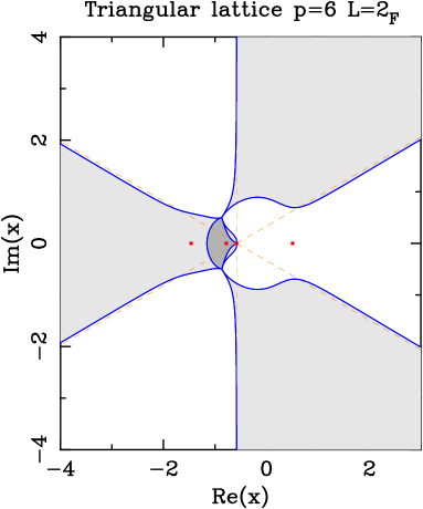
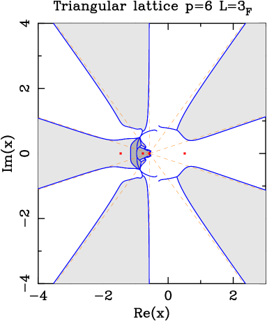
(((a)(a)	(((a)(b)
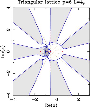
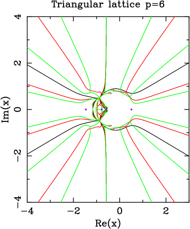
(((a)(c)	(((a)(d)

Figure 11: Limiting curves for the triangular-lattice RSOS model with $p=6$ and several widths: $L=2$ (a), $L=3$ (b), and $L=4$ (c). Figure (d) shows all these curves together: $L=2$ (black), $L=3$ (red), $L=4$ (green). The solid squares $\blacksquare$ show the values where Baxter found the free energy. In the regions displayed in light gray (resp.  white) the dominant eigenvalue comes from the sector $\chi_{1,3}$ (resp. $\chi_{1,1}$). In the regions displayed in a darker gray the dominant eigenvalue comes from the sector $\chi_{1,5}$.

We have computed the limiting curves $\mathcal{B}_{L}$ for $L=2,3,4$. These curves are displayed in Figure 11(a)–(c). In Figure 11(d), we show all three curves for comparison.

5.3.1 $\bm{L=2}$

The transfer matrices are

$${\mathsf{T}}_{1}&=\frac{1}{2}\,\left(\begin{array}[]{cc}x^{4}+2\sqrt{3}x^{3}+6x^{2}+4\sqrt{3}x+3&x\sqrt{2}(x^{3}+2\sqrt{3}x^{2}+4x+\sqrt{3})\\ x^{2}\sqrt{2}(x^{2}+\sqrt{3}x+1)&x^{2}(2x^{2}+2\sqrt{3}x+1)\end{array}\right){}\\ {\mathsf{T}}_{3}=\frac{x}{2}\,\left(\begin{array}[]{ccc}2(x^{3}+2\sqrt{3}x^{2}+4x+\sqrt{3})&\sqrt{2}X_{1}&\sqrt{2}(2x^{3}+4\sqrt{3}x^{2}+7x+\sqrt{3})\\ \sqrt{2}x&X_{2}&X_{2}\\ x\sqrt{2}(2x^{2}+2\sqrt{3}x+1)&X_{2}&4x^{3}+4\sqrt{3}x^{2}+6x+\sqrt{3}\end{array}\right)\\ {}\\ {\mathsf{T}}_{5}=x^{2}{}$$ (5.11)

For real $x$, there are two phase-transition points at

$$x_{{\rm c},1}&=-2/\sqrt{3}\;\approx\;-1.1547005384\\ x_{{\rm c},2}=-1/\sqrt{3}\;\approx\;-0.5773502692$$ (5.12)

The latter one is actually a multiple point. There are also a pair of complex conjugate multiple points at $x=-e^{\pm i\pi/6}=-\sqrt{3}/2\pm i/2$. The dominant sectors on the real $x$-axis are: $\chi_{1,1}$ for $x>-1/\sqrt{3}$, $\chi_{1,3}$ for $x<-2/\sqrt{3}$, and $\chi_{1,5}$ for $x\in(-2/\sqrt{3},-1/\sqrt{3})$.

5.3.2 $\bm{L\geq 3}$

For $L=3$, there are three real phase-transition points at

$$x_{{\rm c},1}&=-2/\sqrt{3}\;\approx\;-1.1547005384\\ x_{{\rm c},2}\approx-0.9712924104\\ x_{{\rm c},3}=-1/\sqrt{3}\;\approx\;-0.5773502692$$ (5.13)

The latter one is actually a multiple point. We have found two pairs of complex conjugate endpoints at $x\approx-0.3495004588\pm 0.6911735024\,i$, and $x\approx-0.2862942369\pm 0.8514701201\,i$. There are 16 pairs of complex conjugate T points. The dominant sectors on the real $x$-axis are $\chi_{1,1}$ for $x>-1/\sqrt{3}$, $\chi_{1,3}$ for $x<-2/\sqrt{3}$, and $\chi_{1,5}$ for $x\in(-2/\sqrt{3},-1/\sqrt{3})$.

For $L=4$, there are five real phase-transition points at

$$x_{{\rm c},1}&=-2/\sqrt{3}\;\approx\;-1.1547005384\\ x_{{\rm c},2}\approx-1.0219801955\\ x_{{\rm c},3}\approx-1.0041094453\\ x_{{\rm c},4}\approx-0.7664034488\\ x_{{\rm c},5}=-1/\sqrt{3}\;\approx\;-0.5773502692$$ (5.14)

The points $x_{{\rm c},3}$ and $x_{{\rm c},4}$ are T points, while $x_{{\rm c},5}$ is a multiple point. We have found a pair of complex conjugate endpoints at $x\approx-0.3857232364\pm 0.6652216322\,i$. In addition, there are 14 pairs of complex conjugate T points. The dominant sectors on the real $x$-axis are

• $\chi_{1,1}$ for $x>x_{{\rm c},4}$

• $\chi_{1,3}$ for $x<-2/\sqrt{3}$ and $x\in(x_{{\rm c},2},x_{{\rm c},3})$

• $\chi_{1,5}$ for $x\in(-2/\sqrt{3},x_{{\rm c},2})\cup(x_{{\rm c},3},x_{{\rm c},4})$

For $L=5$, there are five real phase-transition points at

$$x_{{\rm c},1}&=-2/\sqrt{3}\;\approx\;-1.1547005384\\ x_{{\rm c},2}\approx-0.9326923327\\ x_{{\rm c},3}\approx-0.7350208125\\ x_{{\rm c},4}\approx-0.6186679617\\ x_{{\rm c},5}=-1/\sqrt{3}\;\approx\;-0.5773502692$$ (5.15)

The dominant sectors on the real $x$-axis are

• $\chi_{1,1}$ for $x\in(x_{{\rm c},2},x_{{\rm c},3})\cup(x_{{\rm c},4},\infty)$

• $\chi_{1,3}$ for $x<x_{{\rm c},2}$

• $\chi_{1,5}$ for $x\in(x_{{\rm c},3},x_{{\rm c},4})$

For $L=6$, there are three real phase-transition points at

$$x_{{\rm c},1}&=-2/\sqrt{3}\;\approx\;-1.1547005384\\ x_{{\rm c},2}\approx-1.0504774228\\ x_{{\rm c},3}=-1/\sqrt{3}\;\approx\;-0.5773502692$$ (5.16)

We have also found a small horizontal line belonging to the limiting curve $\mathcal{B}_{6}$ and bounded by the T points

$$x_{{\rm c},4}&\approx-0.7688389273\\ x_{{\rm c},5}\approx-0.7646464215$$ (5.17)

The dominant sectors on the real $x$-axis are

• $\chi_{1,1}$ for $x\in(-1/\sqrt{3},\infty)\cup(x_{{\rm c},4},x_{{\rm c},5})$

• $\chi_{1,3}$ for $x\in(-\infty,-2/\sqrt{3})\cup(x_{{\rm c},2},x_{{\rm c},4})$

• $\chi_{1,5}$ for $x\in(-2/\sqrt{3},x_{{\rm c},2})\cup(x_{{\rm c},5},-1/\sqrt{3})$

In all cases $3\leq L\leq 6$, there is a pair of complex conjugate multiple points at $x=-e^{\pm i\pi/6}$.

5.4 Four-state Potts model ($p=\infty$)

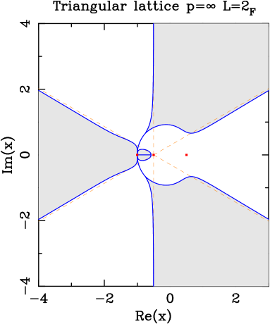
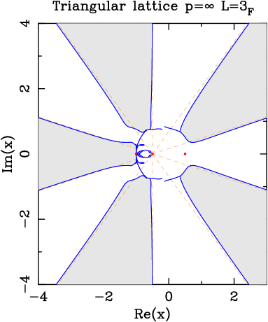
(((a)(a)	(((a)(b)
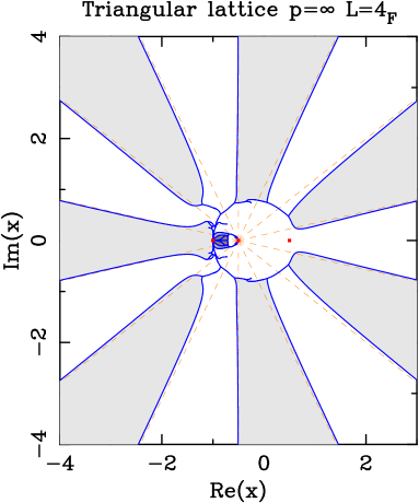
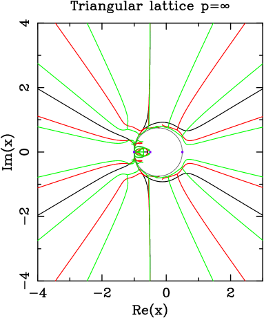
(((a)(c)	(((a)(d)

Figure 12: Limiting curves for the triangular-lattice RSOS model with $p=\infty$ ($Q=4$) and several widths: $L=2$ (a), $L=3$ (b), and $L=4$ (c). Figure (d) shows all these curves together: $L=2$ (black), $L=3$ (red), $L=4$ (green). The solid squares $\blacksquare$ show the values where Baxter found the free energy. In the regions displayed in light gray (resp.  white) the dominant eigenvalue comes from the sector $\chi_{1,3}$ (resp. $\chi_{1,1}$). In regions displayed in a darker gray the dominant eigenvalue comes from the sector $\chi_{1,5}$. In (c), an even darker gray marks the regions with a dominant eigenvalue coming from the sector $\chi_{1,7}$. The gray circle corresponds to (7.8).

We have computed the limiting curves $\mathcal{B}_{L}$ for $L=2,3,4$. These curves are displayed in Figure 12(a)–(c). In Figure 12(d), we show all three curves for comparison.

5.4.1 $\bm{L=2}$

The transfer matrices are

$${\mathsf{T}}_{1}&=\frac{1}{2}\,\left(\begin{array}[]{cc}X_{8}\,(2x^{3}+3x^{2}+6x+4)&\sqrt{3}\,x\,X_{8}\,X_{7}\\ \sqrt{3}\,x^{2}\,X_{7}&x^{2}\,X_{6}\end{array}\right)\\ T_{3}=\frac{1}{6}\,\left(\begin{array}[]{ccc}3xX_{8}(2x^{2}+3x+2)&2\sqrt{6}\,xX_{8}&\sqrt{3}\,xX_{8}X_{6}\\ 2\sqrt{6}\,x^{2}&2x(4+3x)&2\sqrt{2}\,x(2+3x)\\ \sqrt{3}\,x^{2}X_{6}&2\sqrt{2}\,x(3x+2)&xX_{9}\end{array}\right)\\ T_{5}=x^{2}$$ (5.18)

where we have defined the short-hand notations

$$X_{6}&=6x^{2}+9x+2\\ X_{7}=2x^{2}+3x+2\\ X_{8}=x+2\\ X_{9}=18x^{3}+27x^{2}+18x+4$$ (5.19)

For real $x$, we find a multiple point at $x=-1$, and a T point at $x_{c}\approx-0.5808613334$. The limiting curve $\mathcal{B}_{2}$ contains the real interval $[-1,x_{c}]$. At $x=-1$, all eigenvalues become equimodular with $|\lambda_{i}|=1$.

We have found two additional pairs of complex conjugate T points at $x\approx-0.9882427690\pm 0.0896233991\,i$, and $x\approx-3/4\pm 0.6614378278\,i$. The dominant sectors on the real $x$-axis are $\chi_{1,1}$ for $x>x_{c}$, and $\chi_{1,3}$ for $x<x_{c}$. We have found no region in the complex $x$-plane where the sector $\chi_{1,5}$ is dominant.

5.4.2 $\bm{L\geq 3}$

For $L=3$ there are two real phase-transition points: $x=-1$ (which is a multiple point), and $x_{c}\approx-0.8953488450$. The limiting curve contains two connected pieces, two pairs of complex conjugate endpoints, 12 complex conjugate T points, and one additional pair of complex conjugate multiple points at $x\approx-3/4\pm 0.6614378278\,i$. The dominant sectors on the real $x$-axis are $\chi_{1,3}$ for $x<-1$; $\chi_{1,5}$ for $x\in(-1,x_{c})$; and $\chi_{1,1}$ for $x>x_{c}$. We have found no region where the sector $\chi_{1,7}$ is dominant.

For $L=4$ there are two real phase-transition points at $x=-1$ and $x=x_{c}\approx-0.7107999762$, which is a T point. The real line $[-1,x_{c}]$ belongs to the limiting curve. The dominant sectors on the real $x$-axis are: $\chi_{1,3}$ for $x<-1$; $\chi_{1,7}$ for $x\in(-1,x_{c})$; and $\chi_{1,1}$ for $x>x_{c}$. We have found a few small regions with dominant eigenvalue coming from the sector $\chi_{1,5}$; but we have found no region where the sector $\chi_{1,9}$ is dominant.

For $L=5$ there are again two real phase-transition points at $x=-1$ and $x=x_{c}\approx-0.8004698444$, which is a T point. The real line $[-1,x_{c}]$ belongs to the limiting curve. The dominant sectors on the real $x$-axis are: $\chi_{1,3}$ for $x<-1$; $\chi_{1,9}$ for $x\in(-1,x_{c})$; and $\chi_{1,1}$ for $x>x_{c}$.

For $L=6$ there are two real phase-transition points at $x=-1$ and $x=x_{c}\approx-0.7033434642$, which is a T point. The real line $[-1,x_{c}]$ belongs to the limiting curve. The dominant sectors on the real $x$-axis are: $\chi_{1,3}$ for $x<-1$; $\chi_{1,11}$ for $x\in(-1,x_{c})$; and $\chi_{1,1}$ for $x>x_{c}$.

In all cases, the point $x=-1$ is a multiple point where all the eigenvalues are equimodular with $|\lambda_{i}|=1$.

6 Common features of the triangular-lattice limiting curves with free cyclic boundary conditions

The results discussed in Sections 5.1–5.3 allow us to make the following conjecture (in the same spirit as Conjecture 4.1 for the square-lattice case) that states that certain points in the complex $x$-plane belong to the limiting curve $\mathcal{B}_{L}$:

Conjecture 6.1

For the triangular-lattice $Q$-state Potts model with $Q=B_{p}$ and width $L\geq 2$:

1. The points $x=-e^{\pm i\pi/p}$ belong to the limiting curve. At these points, all the eigenvalues are equimodular with $|\lambda_{i}|=1$. Thus, they are in general multiple points.

2. For even $p\geq 6$, the point $x=-2/\sqrt{Q}$ always belongs to the limiting curve $\mathcal{B}_{L}$. Furthermore, if $p=4,6$, then the point $x=-1/\sqrt{Q}$ also belongs to $\mathcal{B}_{L}$.

The phase diagram on the real $x$-axis (which contains the physical regime of the model) shows certain regularities that allow us to make the following conjecture:

Conjecture 6.2

For the triangular-lattice $Q$-state Potts model with $Q=B_{p}$ and width $L\geq 2$:

1. For even $p$, the relevant eigenvalue on the physical line $v\in[-1,\infty)$ comes from the sector $\chi_{1,1}$. For odd $p$, the same conclusion holds for all $L\geq L_{0}$.

2. The relevant eigenvalue belongs to the sector $\chi_{1,3}$ for all real $x<-2/\sqrt{Q}$.

The above conjectures also apply to the limiting case $p\to\infty$ (i.e., $Q=4$). As for the square-lattice case, the multiple points $-e^{\pm i\pi/p}\to-1$ as $p\to\infty$ (Conjecture 6.1.1) in agreement with the fact that $x=-1$ is a multiple point for $Q=4$. Furthermore, this is also in agreement with Conjecture 6.1.2, as in this limit, $-2/\sqrt{Q}=-1$. The dominant sectors for $p\to\infty$ also agree with Conjecture 6.2: on the physical line $v\in[-1,\infty)$ the dominant sector is $\chi_{1,1}$, and for $x<-1$, the dominant sector is $\chi_{1,3}$. More precisely, we can state the following conjecture based on the empirical observations reported above:

Conjecture 6.3

For the triangular-lattice $4$-state Potts model defined on a semi-infinite strip of width $L\geq 2$, there exists some $x_{c}(L)>-1$ such that $\chi_{1,1}$ is dominant for $x>x_{c}(L)$, $\chi_{1,2L-1}$ is dominant for $-1<x<x_{c}(L)$, $\chi_{1,3}$ is dominant for $x<-1$.

6.1 Asymptotic behavior for $\bm{|x|\to\infty}$

Figures 9–12 show a similar scenario to the one discussed in Section 4: There are several unbounded outward branches with a clear asymptotic behavior for large $|x|$. Again, this scenario also holds in the limit $p\to\infty$ (See Figure 12). However there are quantitative differences with the scenario found for the square lattice. We should modify Conjecture 4.5 as follows:

Conjecture 6.4

Let $\lambda_{\star,1}(L)$ (resp. $\lambda_{\star,3}$(L)) be the leading eigenvalue of the sector $\chi_{1,1}$ (resp.  $\chi_{1,3}$) in the regime $|x|\to\infty$. Then

$$\lambda_{\star,1}(L)&=Q^{L-1}\,x^{3L-2}\,\left[1+\sum\limits_{k=1}^{\infty}\frac{b_{k}(L)}{Q^{k/2}}\,x^{-k}\right]\\ \lambda_{\star,1}(L)-\lambda_{\star,3}(L)=2^{L-1}\sqrt{Q}\,x^{L-1}+(L-1)\,2^{L-1}\,x^{L-2}+O(x^{L-3})$$ (6.1)

Furthermore, we have that

$$b_{1}(L)&=3L-2\,,\qquad L\geq 2\\ b_{2}(L)=\frac{9}{2}L^{2}-\frac{15}{2}L+3\,,\qquad L\geq 2\\ b_{3}(L)=\frac{9}{2}L^{3}-\frac{27}{2}L^{2}+13L-4\,,\qquad L\geq 3$$ (6.2)

The first coefficients $b_{k}(L)$ are displayed in Table 2; the patterns displayed in (6.2) are easily verified. The coefficients $b_{k}(L)$ also depend on $p$ for $k\geq 4$.

Conjecture 6.4 explains the number of outward branches in the triangular-lattice case, as well as the observed pattern for the outward branches. Again, these branches are defined by the equimodularity of the two leading eigenvalues

$$|\lambda_{\star,1}|\;=\;|\lambda_{\star,3}|\;=\;\left|\lambda_{\star,1}-\text{const.\ }x^{L-1}+O(x^{L-2})\right|$$ (6.3)

This implies that

$$\mathop{\rm Re}\nolimits\left[\lambda_{\star,1}\overline{x}^{L-1}\right]\;=\;0$$ (6.4)

Then, if $x=|x|e^{i\theta}$, the above equation reduces to

$$\cos\left(\theta(2L-1)\right)\;=\;0\;\Rightarrow\;\theta_{n}=\frac{\pi}{2(2L-1)}(2n-1)\,,\quad n=1,2,\dots,2(2L-1)$$ (6.5)

Thus, we get the same asymptotic behavior as for the square lattice with the replacement $L\to 2L-1$.

7 Discussion of the results with free cyclic boundary conditions

The results obtained give indications on the phase diagram of the Potts model, as the accumulating points of the zeros of the partition function correspond to singularities of the free energy.

Extrapolating the curves obtained to $L\to\infty$ in not an easy matter, given that we have only access to relatively small $L$. However, in Sections 4 and 6 we have noted a number of features which hold for all $L$ considered, and hence presumably for all finite $L$ and also in the thermodynamic limit.

7.1 Ising model

The most transparent case is that of the Ising model ($p=4$) on the square lattice. Let $D(x,r)$ denote the disk centered in $x$ and of radius $r$. There are then four different domains of interest:

$$\mathcal{D}_{1}&\;=\;D(0,1)\setminus D(-\sqrt{2},1)\\ \mathcal{D}_{2}\;=\;D(0,1)\cap D(-\sqrt{2},1)\\ \mathcal{D}_{3}\;=\;D(-\sqrt{2},1)\setminus D(0,1)\\ \mathcal{D}_{4}\;=\;{\mathbb{C}}\setminus\left(D(0,1)\cup D(-\sqrt{2},1)\right)$$ (7.1)

The $L\times N$ strips with even $N$ are bipartite, whence the Ising model possesses the exact gauge symmetry $J\to-J$ (change the sign of the spins on the even sublattice). Since the limit $N\to\infty$ can be taken through even $N$ only, the limiting curves $\mathcal{B}_{L}$ should be gauge invariant. In terms of $x$ the gauge transformation reads

$$x\to-\frac{x}{1+x\sqrt{2}}\,.$$ (7.2)

Note that it exchanges $\mathcal{D}_{2}\leftrightarrow\mathcal{D}_{4}$, while leaving $\mathcal{D}_{1}$ and $\mathcal{D}_{3}$ invariant. In particular, the structures of $\mathcal{B}_{L}$ around $x=-1/\sqrt{2}$ and $|x|=\infty$ discussed in Section 4 are equivalent.

On the other hand, the duality transformation $x\to 1/x$ is not a symmetry of $\mathcal{B}_{L}$: this is due to the fact that the boundary conditions prevent the lattice from being selfdual. Note that the duality exchanges $\mathcal{D}_{1}\leftrightarrow\mathcal{D}_{4}$ and $\mathcal{D}_{2}\leftrightarrow\mathcal{D}_{3}$. But whilst there are many branches of $\mathcal{B}_{L}$ in $\mathcal{D}_{4}$, there are none in $\mathcal{D}_{1}$.

The Ising model being very simple, we do however expect the fixed point structure on the real $x$-axis to satisfy duality. Combining the gauge and duality transformations one can connect all critical fixed points:

$$x_{\text{FM}}\;\stackrel{{\scriptstyle\rm gauge}}{{\longrightarrow}}\;x_{+}\;\stackrel{{\scriptstyle\rm duality}}{{\longrightarrow}}\;x_{-}\;\stackrel{{\scriptstyle\rm gauge}}{{\longrightarrow}}\;x_{\text{BK}},$$ (7.3)

and the first and the last points in the series are selfdual. In the same way, all the non-critical (trivial) fixed points are connected:

$$x=0\;\stackrel{{\scriptstyle\rm duality}}{{\longrightarrow}}\;|x|=\infty\;\stackrel{{\scriptstyle\rm gauge}}{{\longrightarrow}}\;x=-1/\sqrt{2}\;\stackrel{{\scriptstyle\rm duality}}{{\longrightarrow}}\;x=-\sqrt{2},$$ (7.4)

and the first and the last points in the series are gauge invariant.

The reason that we discuss these well-known facts in detail is that the square-lattice Ising model is really the simplest example of how taking $p$ rational (here, in fact, integer) profoundly modifies and enriches the fixed/critical point structure of the Potts model, as compared to the generic case of $p$ irrational. Taking the limit $p\to 4$ through irrational values we would have had three equivalent $c=1/2$ critical points, RG repulsive in $x$, situated at $x_{\text{FM}}$ and $x_{\pm}$; one $c=-25/2$ critical point, RG attractive in $x$, situated at $x_{\text{BK}}$; and two non-critical (trivial) fixed points, RG attractive in $x$, situated at $x=0$ and $|x|=\infty$. This makes up for a phase diagram on the real $x$-axis which is consistent in terms of renormalization group flows (see the top part of Fig. 2).

Conversely, sitting directly at $p=4$ replaces this structure by the four repulsive $c=1/2$ critical points (7.3) and the four attractive non-critical fixed points (7.4). This again gives a consistent scenario, in which notably the BK phase has disappeared (see the bottom part of Fig. 2). In other cases than the Ising model ($p>4$ integer) we could expect the emergence of even more new (as compared to the case of irrational $p$) fixed points (critical or non-critical), which will in general be inequivalent (due in particular to the absence of the Ising gauge symmetry).

Going back to the case of complex $x$ we can now conjecture:

Conjecture 7.1

Let $\mathcal{D}_{1}$ be the domain defined in Eq. (7.1d). Then

• The points $x$ such that

  $$Z_{L_{\rm F}\times N_{\rm P}}(Q=2;x)=0\quad(\text{\rm square lattice})$$ (7.5)

  for some $L$ and $N$ are dense in ${\mathbb{C}}\setminus\mathcal{D}_{1}$.

• There are no such points in $\mathcal{D}_{1}$.

We now turn to the Ising model on the triangular lattice. We first note that all the limiting curves $\mathcal{B}_{L}$ are symmetric under the combined transformation $x\leftrightarrow-x-\sqrt{2}$ and $\chi_{1,1}\leftrightarrow\chi_{1,3}$. On the level of the coupling constant this can also be written $\exp(J)\to-\exp(J)$.

We also conjecture that

Conjecture 7.2

Let $\mathcal{D}_{\rm tri}$ be the interior of the ellipse

$$\left(\mathop{\rm Re}\nolimits x+1/\sqrt{2}\right)^{2}+3\left(\mathop{\rm Im}\nolimits x\right)^{2}=3/2\,.$$ (7.6)

Then

• The points $x$ such that

  $$Z_{L_{\rm F}\times N_{\rm P}}(Q=2;x)=0\quad(\text{\rm triangular lattice})$$ (7.7)

  for some $L$ and $N$ are dense in ${\mathbb{C}}\setminus\mathcal{D}_{\rm tri}$.

• There are no such points in $\mathcal{D}_{\rm tri}$.

7.2 Models with $p>4$

For square-lattice models with $p>4$ the phase diagram in the thermodynamic limit is expected to be more complicated. We can nevertheless conjecture that the four values $x_{\rm c}$ given by Eq. (1.4), and denoted by solid squares in the figures, correspond to phase transition points even for $Q=B_{p}$ a Beraha number. Accordingly, these points are expected to be accumulation points for the limiting curves $\mathcal{B}_{L}$, when $L\to\infty$.

But these four values of $x$ are not the only fixed points. There is a complex fixed point structure between $x_{-}(Q)$ and $x_{\rm BK}(Q)$, and between $x_{\rm BK}(Q)$ and $x_{+}(Q)$. This is because for $Q$ equal to a Beraha number, the thermal operator is repulsive at $x_{\rm BK}(Q)$ (and not attractive as it would have been in the BK phase for irrational $p$), whereas it remains repulsive at $x_{-}(Q)$ and $x_{+}(Q)$. Therefore, there must at the very least be one attractive fixed point in each of the two intervals mentioned, in order for a consistent phase diagram to emerge. Indeed, for $p$ even, there are two new fixed points, one of them being conjectured as $-\sqrt{Q}/2$ for all even $p$, and the other being equal to $-\sqrt{Q}$ only for $p=4$ and $p=6$. But our results for finite $L$ are in favor of an even more complicated structure, involving more new fixed points. The structure of the phase diagram for $p$ odd is further complicated by the emergence of segments of the real $x$-axis belonging to $\mathcal{B}_{L}$. It is however uncertain, whether these segments will stay of finite length in the $L\to\infty$ limit.

In the models with $p=5,6,\infty$ and on both the square and triangular lattices, we have found strong numerical evidence to conjecture that the partition-function zeros are dense in the whole complex $x$-plane with the exception of the interior of some domain. The shape of this domain depends on both $p$ and the lattice structure; and unlike in the Ising case ($p=4$), we do not have enough evidence to conjecture its algebraic expression [c.f., Conjectures 7.1 and 7.2]. For the square lattice and fixed $p$, the limiting curves $\mathcal{B}_{L}$ seem to approach (from the outside) the circles (1.5), especially in the ferromagnetic regime $\mathop{\rm Re}\nolimits x\geq 0$. For the triangular lattice and $p=\infty$, the limiting curves in Figure 12 seem to approach the circle

$$\left(\mathop{\rm Re}\nolimits x+\frac{1}{4}\right)^{2}+(\mathop{\rm Im}\nolimits x)^{2}\;=\;\left(\frac{3}{4}\right)^{2}$$ (7.8)

which goes through the bulk critical points $x=-1$ and $x=1/2$.

7.3 The region $|x|\gg 1$

The emergence of unbounded branches of $\mathcal{B}_{L}$ in the region of $|x|\gg 1$ is at first sight rather puzzling. Because when $|x|$ is large enough, we should expect the system to be non-critical, and thus be described by a unique leading eigenvalue of the transfer matrix. This is at least what happens for the $q$-state Potts model on a strip with cylindrical or free boundary conditions using the Fortuin–Kasteleyn representation [39, 40].

One of the main reasons for studying the limiting curves in the first place is that we wish to use them to detect the critical points of the models at hand. At a conformally invariant critical point there should be an infinite spectrum of transfer-matrix eigenvalues $|\Lambda_{0}|\geq|\Lambda_{1}|\geq\ldots$ that become degenerate according to [46] $|\Lambda_{i}/\Lambda_{0}|\sim\exp(-2\pi x_{i}/L)$ when $L\to\infty$, where $x_{i}$ are critical exponents. The limiting curves just tell us that the two dominant eigenvalues become degenerate, and not even with what finite-size corrections. Therefore the fact that a point $x$ (even on the real axis) is an accumulation point of $\mathcal{B}_{L}$ is not sufficient for $x$ to be a critical point in the sense of the above scaling behavior.

The observed behavior for $|x|\gg 1$ just shows that the leading eigenvalues in sectors with different boundary conditions ($\chi_{1,1}$ and $\chi_{1,3}$) come close. This is most transparent in the Ising case, where there is a bijection between RSOS heights and dual spins. It is easily seen that $\chi_{1,1}$ (resp. $\chi_{1,3}$) corresponds to fixed boundary conditions in the spin representation, with all the dual spins on the upper/lower rim being fixed as $+/+$ (resp. $+/-$). On the other hand, within a given sector there should be a finite gap between the leading and next-leading eigenvalues, in the region $|x|\gg 1$, signaling non-critical behavior.

7.4 Fixed cyclic boundary conditions

To avoid the (from the point of view of detecting critical behavior) spurious coexistence between two different boundary conditions, we should rather pick boundary conditions that break the $Z_{Q}$ symmetry of the $Q$-state Potts model explicitly. We now illustrate this possibility by making a particular choice of fixed boundary conditions, which has the double advantage of generalizing those for the Ising case (as discussed above) and enabling the corresponding Potts model partition function $Z_{L_{\rm X}\times N_{\rm P}}(Q;v)$ to be written as a sum of RSOS model partition functions.

Consider first the Potts model partition function $\tilde{Z}$ on the dual lattice, with spins $S_{+}$ and $S_{-}$ on the upper and lower exterior dual sites, and at the dual coupling $\tilde{J}$. Recall that the duality relation reads simply $v\tilde{v}=Q$. If we impose free boundary conditions on $S_{\pm}$, we have by the fundamental duality relation [1]

$$Q^{V-E/2-1}x^{E}\tilde{Z}(Q;Q/v)=Z(Q;v),$$ (7.9)

where $E$ (resp. $V$) is the total number of lattice edges (resp. direct sites). Note that $V=LN$, and that $E=2V-N$ (resp. $E=3V-2N$) for the square (resp. triangular) lattice. We now claim that this object with fixed and equal values for $S_{\pm}$ can again be expressed in terms of $K_{1,2j+1}$, for a generic $p$. The precise relation reads

$$Z_{L_{\rm X}\times N_{\rm P}}(Q;v)\equiv Q^{V-E/2}x^{E}\left.\tilde{Z}(Q;Q/v)\right|_{S_{+}=S_{-}}=Q^{LN/2}\sum_{j=0}^{L}\beta_{j}(p)\,K_{1,2j+1}(p,L;x),$$ (7.10)

which should be compared with Eq. (2.3). We henceforth refer to $Z_{L_{\rm X}\times N_{\rm P}}(Q;v)$ as the partition function of the Potts model with fixed cyclic boundary conditions (even though it would be more precise to say that it is actually the two exterior dual spins that get fixed). The amplitudes read

$$\beta_{j}(p)=\frac{S_{j}(p)}{Q}+(-1)^{j}\left(1-\frac{1}{Q}\right)\;.$$ (7.11)

Note that for arbitrary values of $Q$, the partition function $\left.\tilde{Z}(Q;Q/v)\right|_{S_{+}=S_{-}}$ can be defined by its FK cluster expansion on the dual lattice, by giving a weight $Q$ to clusters that do not contain any of the two exterior sites, and a weight $1$ to clusters containing at least one of two exterior sites. Eq. (7.10) is a special case of a more general relation which will be proved and discussed elsewhere.

Now, for $p$ integer, we would like to express $Z_{L_{\rm X}\times N_{\rm P}}(Q;v)$ in terms of the $\chi_{1,2j+1}(p,L;x)$ as we did in the case of free cyclic boundary conditions. But because of the $(-1)^{j}$ in the expression of $\beta_{j}(p)$, we have $\beta_{np+j}(p)=\beta_{j}(p)$ and $\beta_{(n+1)p-1-j}=-\beta_{j}$, cf. Eq. (2.4) for the case of $S_{j}(p)$, only if $p$ is even. For $p$ even, we can express

$$Z_{L_{\rm X}\times N_{\rm P}}(Q;v)=Q^{LN/2}\sum_{j=0}^{\lfloor(p-2)/2\rfloor}\beta_{j}(p)\,\chi_{1,2j+1}(p,L;x)\qquad(p\ \mbox{even})$$ (7.12)

which should be compared with Eq. (2.5). For $p$ odd, there does not appear to exist an expansion of $Z_{L_{\rm X}\times N_{\rm P}}$ in terms of $\chi_{1,2j+1}$.

Note in particular that $\beta_{1}(p)=0$ for any $p$. This has the consequence of eliminating the $\chi_{1,3}$ sector from the partition function, and, as we now shall see, modify the $|x|\gg 1$ behavior of the phase diagram.

8 Square-lattice Potts model with fixed cyclic boundary conditions

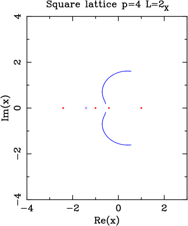
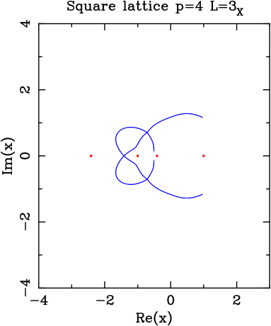
(((a)(a)	(((a)(b)
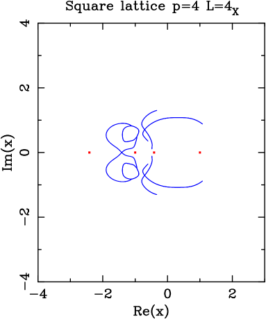
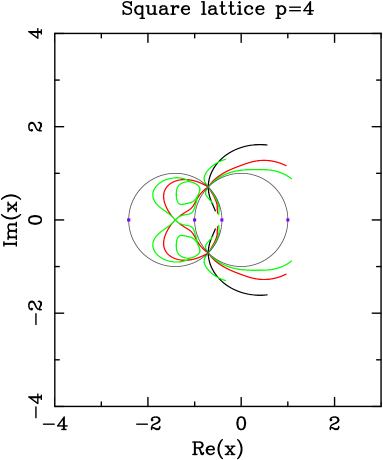
(((a)(c)	(((a)(d)

Figure 13: Limiting curves for the square-lattice RSOS model with $p=4$ and several widths: $L=2$ (a), $L=3$ (b), and $L=4$ (c) when only the sector $\chi_{1,1}$ is taken into account. Figure (d) shows all these curves together: $L=2$ (black), $L=3$ (red), $L=4$ (green). The solid squares $\blacksquare$ show the values where Baxter found the free energy. The dark gray circles correspond to (1.5)

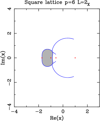
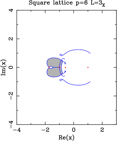
(((a)(a)	(((a)(b)
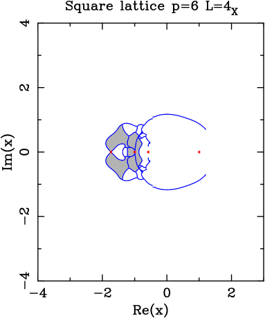
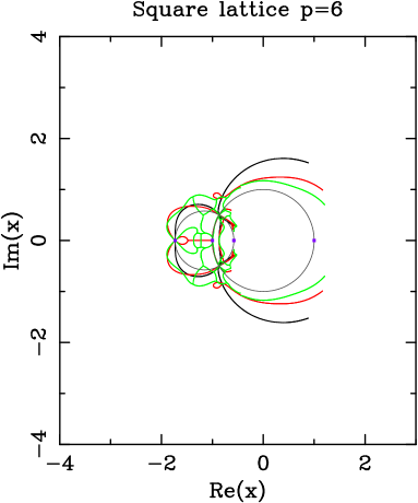
(((a)(c)	(((a)(d)

Figure 14: Limiting curves for the square-lattice RSOS model with $p=6$ and several widths: $L=2$ (a), $L=3$ (b), and $L=4$ (c) when only the sectors $\chi_{1,1}$ and $\chi_{1,5}$ are taken into account. In the regions displayed in dark gray (resp.  white) the dominant eigenvalue comes from the sector $\chi_{1,5}$ (resp. $\chi_{1,1}$). Figure (d) shows all these curves together: $L=2$ (black), $L=3$ (red), $L=4$ (green). The solid squares $\blacksquare$ show the values where Baxter found the free energy. The dark gray circles correspond to (1.5)

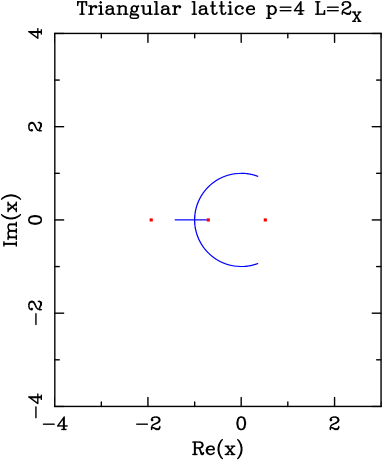
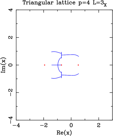
(((a)(a)	(((a)(b)
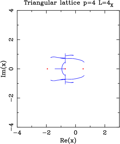
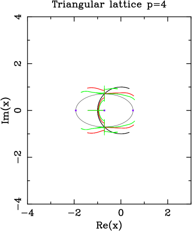
(((a)(c)	(((a)(d)

Figure 15: Limiting curves for the triangular-lattice RSOS model with $p=4$ and several widths: $L=2$ (a), $L=3$ (b), and $L=4$ (c) when only the sector $\chi_{1,1}$ is taken into account. Figure (d) shows all these curves together: $L=2$ (black), $L=3$ (red), $L=4$ (green). The gray ellipse corresponds to $(\mathop{\rm Re}\nolimits x+1/\sqrt{2})^{2}+3(\mathop{\rm Im}\nolimits x)^{2}=3/2$. This curve goes through the points $x=-e^{\pm i\,\pi/4}$.

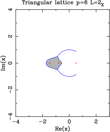
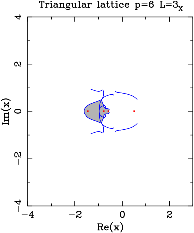
(((a)(a)	(((a)(b)
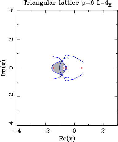
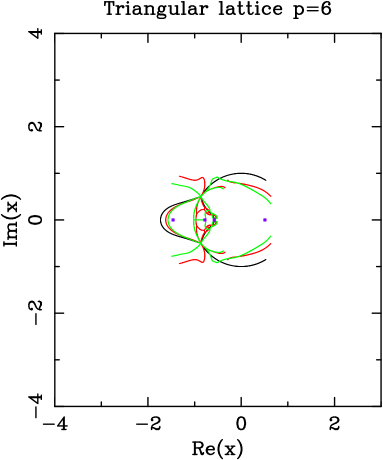
(((a)(c)	(((a)(d)

Figure 16: Limiting curves for the triangular-lattice RSOS model with $p=6$ and several widths: $L=2$ (a), $L=3$ (b), and $L=4$ (c) when only the sectors $\chi_{1,1}$ and $\chi_{1,5}$ are taken into account. In the regions displayed in dark gray (resp.  white) the dominant eigenvalue comes from the sector $\chi_{1,5}$ (resp. $\chi_{1,1}$). Figure (d) shows all these curves together: $L=2$ (black), $L=3$ (red), $L=4$ (green). The solid squares $\blacksquare$ show the values where Baxter found the free energy.

The limiting curves $\mathcal{B}_{L}$ with fixed cyclic boundary conditions (see Figs. 13–16) are very similar to those obtained in Ref. [39] for the Potts model with fully free boundary conditions. On the other hand, we have already seen that the $\mathcal{B}_{L}$ with free cyclic boundary conditions are very different.

Before presenting the results for fixed cyclic boundary conditions in detail we wish to explain this similarity. We proceed in two stages. First we present an argument why the limiting curves corresponding to just the sector $\chi_{1,1}$ almost coincide with those for fully free boundary conditions. Second, we take into account the effect of adding other sectors $\chi_{1,2j+1}$.

Let ${\mathsf{T}}_{\rm FK}$ be the transfer matrix in the FK representation with zero bridges (cf. footnote 6), and let $\lambda_{i}$ be its eigenvalues. Then one has, with cyclic boundary conditions

$$K_{1,1}=\mathop{\rm tr}\nolimits{\mathsf{T}}_{\text{FK}}^{N}=\sum_{i}\lambda_{i}^{N}.$$ (8.1)

Due to the coupling of $K_{1,2j+1}$, given by Eq. (2.6), the eigenvalues of ${\mathsf{T}}_{1}$ (i.e., the transfer matrix that generates $\chi_{1,1}$, cf. Eq. (2.8)) form only a subset of the eigenvalues of ${\mathsf{T}}_{\rm FK}$. More precisely,

$$\chi_{1,1}=\sum_{i}\tilde{\alpha}_{i}\lambda_{i}^{N},$$ (8.2)

where $\tilde{\alpha}_{i}=0$ or $1$ are independent of $x$. Note that when $L<p-1$, Eq. (2.6) gives simply $\chi_{1,1}=K_{1,1}$, and so in that case all $\tilde{\alpha}_{i}=1$.

Meanwhile, the partition function of the Potts model with fully free boundary conditions is given by [32]

$$Z_{\text{free}}=\langle f|{\mathsf{T}}_{\rm FK}^{N}|i\rangle=\sum\limits_{i\geq 1}\alpha_{i}\,\lambda_{i}^{N},$$ (8.3)

where the amplitudes $\alpha_{i}$ are due to the free longitudinal boundary conditions. Note that some of the $\alpha_{i}$ could vanish identically, and indeed many of them do vanish. For example, in the case of the square lattice, the vectors $|i\rangle$ and $\langle f|$ are symmetric under a reflection with respect to the axis of the strip, whence only the $\lambda_{i}$ corresponding to eigenvectors which are symmetric under this reflection will contribute to $Z_{\text{free}}$.

For $x>0$ real and positive, it follows from simple probabilistic arguments that the dominant eigenvalue $\lambda_{0}$ will reside in the zero-bridge sector $K_{1,1}$ and is not canceled by eigenvalues coming from other sectors. Therefore $\tilde{\alpha}_{0}=1$. On the other hand, the Perron-Frobenius theorem and the structure of the vectors $|i\rangle$ and $\langle f|$ implies that $\alpha_{0}>0$. We conclude that the dominant term in the expansions of $\chi_{1,1}$ and $Z_{\rm free}$ are proportional. By analytic continuation the same conclusion holds true in some domain in the complex $x$-plane containing the positive real half-axis. Moving away from that half-axis, a first level crossing will take place when $\lambda_{0}$ crosses another eigenvalue $\lambda_{i}$. If none of the functions $\alpha_{i}$ and $\tilde{\alpha}_{i}$ are identically zero, the corresponding branch of the limiting curve $\mathcal{B}_{L}$ coincides in the two cases. Further away from the positive real half-axis other level crossings may take place, and the limiting curves remain identical until a level crossing between $\lambda_{j}$ and $\lambda_{k}$ takes place in which either $\alpha_{j}=0$ and $\tilde{\alpha}_{j}\neq 0$, or conversely $\alpha_{j}\neq 0$ and $\tilde{\alpha}_{j}=0$. When $L<p-1$ the only possibility is the former one, since all $\tilde{\alpha}_{i}=1$.

If we now compare the limiting curves of $Z_{\text{free}}$ and $Z_{\text{RSOS}}$, the latter being defined as some linear combination of $\chi_{1,2j+1}$ (containing $\chi_{1,1}$), the above argument will be invalidated if the first level crossing in $Z_{\text{RSOS}}$ when moving away from the positive half-axis involves an eigenvalue from $\chi_{1,2j+1}$ with $j>0$.

With free cyclic boundary conditions, $Z_{\text{RSOS}}$ contains $\chi_{1,3}$. The first level crossing involves eigenvalues from $\chi_{1,1}$ and $\chi_{1,3}$ (cf. the observed unbounded branches) and is situated very “close” [cf. Eqs. (4.7) and (6.5) with $n=1$] to the positive real half-axis. Accordingly, the limiting curves $\mathcal{B}_{L}$ do not at all resemble those with fully free boundary conditions. On the other hand, when $\chi_{1,3}$ is excluded (i.e., in the case of fixed cyclic boundary conditions) the first level crossing is between two different eigenvalues from the $\chi_{1,1}$ sector (see Figs. 13–16).

8.1 Ising model ($p=4$)

We have studied the limiting curves given by the sector $\chi_{1,1}$ in the square-lattice Ising case. The results are displayed in Figure 13. It is clear that there are no outward branches, as there is a unique dominant eigenvalue in the region $|x|\gg 1$. Indeed, this agrees with the expected non-critical phase. These curves are very similar to those obtained using the Fortuin-Kasteley representation for a square-lattice strip with free boundary conditions [39]. In particular, for even $L=2,4$ we find that these curves do in fact coincide. However, for $L=3$ we find disagreements; but only in the region $\mathop{\rm Re}\nolimits v<-1$. Namely, the complex conjugate closed regions defined by the multiple points $x=-e^{-i\pi/4}$ and $x=-\sqrt{2}$ (see Figure 13b) are replaced by two complex conjugate arcs emerging from $x=-e^{-i\pi/4}$. These arcs bifurcate at two complex conjugate T points.

For $L=2$ we find two pairs of complex conjugate endpoints at $x\approx-0.5558929703\pm 0.1923469388\,i$, and $x\approx 0.5558929703\pm 1.6065605012\,i$. There is a double endpoint at $x=-\sqrt{2}$.

For $L=3$ we also find two pairs of complex conjugate endpoints at $x\approx-0.5054436896\pm 0.1404486742\,i$, and $x\approx 0.9624601506\pm 1.1627733180\,i$. There is a multiple point at $q=-\sqrt{2}$, and a pair of complex conjugate multiple points at $q=-e^{-\pm\pi i/4}$. These multiple points also appear in $L=4$.

For $L=4$ we find two connected components in the limiting curve. There are two pairs of complex conjugate T points at $q\approx-1.1111427356\pm 0.8231882219\,i$, and $q\approx-0.9473515724\pm 0.4894779296\,i$. We also find four complex conjugate pairs of endpoints at $q\approx-0.6052879436\pm 0.3554255102\,i$, $q\approx-0.4820292937\pm 0.1111133833\,i$, $q\approx-0.3346743307\pm 1.3000737077\,i$, and $q\approx 1.0790506924\pm 0.8817674400\,i$.

8.2 Three-state Potts model ($p=6$)

We have studied the limiting curves given by the sectors $\chi_{1,1}$ and $\chi_{1,5}$, cf. Eq. (7.12). The results are displayed in Figure 14. We have compared these curves with those obtained for a square-lattice strip with free boundary conditions [39]. We find that they agree almost perfectly in the region $\mathop{\rm Re}\nolimits x\geq-1$. The only exceptions are the tiny complex conjugate branches emerging from the multiple points $-e^{-i\pi/6}$ for $L=3,4$ and pointing to $x_{\text{BK}}$. The differences are in both cases rather small and they are away from the real $x$-axis. In the region $\mathop{\rm Re}\nolimits x<-1$, however, the differences between the two boundary conditions are sizeable. For free boundary conditions the closed regions tend to disappear, or, at least, to diminish in number and size.

9 Triangular-lattice Potts model with fixed cyclic boundary conditions

9.1 Ising model ($p=4$)

We have studied the limiting curves given by the sector $\chi_{1,1}$ in the triangular-lattice Ising case. The results are displayed in Figure 15, and they are the same than those obtained with the Fortuin-Kasteleyn representation [40], with free boundary conditions, for all $L$. Therefore, we see a non-trivial effect of the lattice: for the triangular lattice, the dominant eigenvalues always comes from $K_{1,1}$, contrary to the case of the square lattice.

For $L=2$ we find two real endpoints at $q=-\sqrt{2}$ and $q=-1/\sqrt{2}$, and an additional pair of complex conjugate endpoints at $x\approx 0.3535533906\pm 0.9354143467\,i$. At $x=-1$ there is a crossing between the two branches of the limiting curve.

For $L=3$ we find two real endpoints at $q=-\sqrt{2}$ and $q=-1/\sqrt{2}$, and four pairs of complex conjugate endpoints at $x\approx-1.4346151869\pm 0.9530458628\,i$, $x\approx 0.5477064083\pm 0.6206108204\,i$, $x\approx-1/\sqrt{2}\pm 0.4918781633\,i$, and $x\approx-1/\sqrt{2}\pm 0.9374415716\,i$. The limiting curve contains two complex conjugate vertical lines determined by the latter two pairs of endpoints, and a horizontal line determined by the two real endpoints. We have found three pairs of complex conjugate T points at $x\approx-1\sqrt{2}\pm 0.5353475100\,i$, $x\approx-1\sqrt{2}\pm 0.7246267519\,i$, and $x\approx-1\sqrt{2}\pm 0.8539546894\,i$. Finally, there is a multiple point at $x\approx-0.9681295813$.

For $L=4$, we again find a horizontal real line bounded by two real endpoints at $x=-\sqrt{2}$, and $x=-1/\sqrt{2}$, and a pair of complex conjugate vertical lines bounded by the endpoints $x\approx-1\sqrt{2}\pm 1.0514178378\,i$, and $x\approx-1\sqrt{2}\pm 0.3816638845\,i$. We have found and additional pair of endpoints at $x\approx 0.5890850526\pm 0.4519358255\,i$. There are five pairs of T points; two of them are located on the line $\mathop{\rm Re}\nolimits x=-1\sqrt{2}$. These are $x\approx-1\sqrt{2}\pm 0.4336035301\,i$, and $x\approx-1\sqrt{2}\pm 0.7394246716\,i$. The other three pairs are $x\approx-1.0712333535\pm 0.7555078808\,i$, $x\approx-1.6123945698\pm 0.8042942359\,i$, and $x\approx-0.3186094544\pm 0.9388965869\,i$. We find four bulb-like regions around the latter two pairs of T points. Finally, there is a multiple point at $x\approx-0.9415556904$, and a complex conjugate pair of multiple points at $q=-e^{\pm i\pi/4}$.

We have compared the above-described limiting curves with those of a triangular-lattice model with free boundary conditions [40]. The agreement is perfect on the whole complex $x$-plane for $L=2,3,4$.

9.2 Three-state Potts model ($p=6$)

We have studied the limiting curves given by the sectors $\chi_{1,1}$ and $\chi_{1,5}$, cf. Eq. (7.12). The results are displayed in Figure 16. As for the square-lattice case discussed in Section 8.2, the limiting curves coincide with those obtained with free boundary conditions in a domain containing the real positive $v$-axis. In particular, the agreement is perfect in the first regime $\mathop{\rm Re}\nolimits v\geq 0$. In the second regime $-1\leq\mathop{\rm Re}\nolimits v\leq 0$, the coincidence holds except on a small region close to $\mathop{\rm Re}\nolimits v=-1$, and $|\mathop{\rm Im}\nolimits v|$ small for $L=3,4$. In both cases, the branches that emerge from $x=-1/\sqrt{3}$ and penetrate inside the second regime (and defining a closed region), change their shape for free boundary conditions (and in particular, the aforementioned closed regions are no longer closed). Finally, in the third regime $\mathop{\rm Re}\nolimits v<-1$, the limiting curves for both types of boundary conditions clearly differ. As for the square-lattice three-state model, free boundary conditions usually imply less and smaller closed regions.

10 Conclusion and outlook

We have studied the complex-temperature phase diagram of the $Q$-state Potts model on the square and triangular lattices with $Q=4\cos^{2}(\pi/p)$ and $p$ integer. The boundary conditions were taken to be cyclic so as to make contact with the theory of quantum groups [24, 27, 28, 6, 7], which provides a framework for explaining how a large amount of the eigenvalues of the cluster model transfer matrix—defined for generic values of $p$—actually do not contribute to the partition function $Z$ for $p$ integer. Moreover, for $p$ integer, the exact equivalence (2.5) between the Potts and the $A_{p-1}$ RSOS model provides an efficient way of computing exactly those eigenvalues that do contribute to $Z$. Using the Beraha-Kahane-Weiss theorem [30], this permitted us to compute the curves $\mathcal{B}_{L}$ along which partition function zeros for cyclic strips of finite width $L$ accumulate when the length $N\to\infty$.

The RSOS model has the further advantage of associating a quantum number $j$ with each eigenvalue, which is related to the number of clusters of non-trivial topology with respect to the periodic direction of the lattice and to the spin $S_{z}$ of the associated six-vertex model. This number then characterizes each of the phases (enclosed regions) defined by $\mathcal{B}_{L}$.

The curves $\mathcal{B}_{L}$ turn out to exhibit a remarkable regularity in $L$—at least in some respects—thus enabling us to make a number of conjectures about the thermodynamic limit $L\to\infty$. On the other hand, even a casual glance at the many figures included in this paper should convince the reader that the $L\to\infty$ limit of the models at hand might well conceal many complicated features and exotic phase transitions. Despite of these complications, we venture to summarize our essential findings, by regrouping them in the same way as in the list of open issues presented in the Introduction:

1. The points $x_{\rm FM}(Q)$ and $x_{-}(Q)$ (and for the square lattice also its dual $x_{+}(Q)$), that act as phase transition points in the generic phase diagram, should play a similar role for integer $p$. This can be verified from the figures in which it is more-or-less obvious that the corresponding red solid squares will be traversed, or pinched, by branches of $\mathcal{B}_{L}$ in the $L\to\infty$ limit. What is maybe more surprising is that also $x_{\rm BK}(Q)$ has a similar property, despite of the profoundly changed physics inside the BK phase. Indeed, in most cases, $x_{\rm BK}(Q)$ is either exactly on or very close to a traversing branch of $\mathcal{B}_{L}$. It remains an open question to characterize exactly the nature of the corresponding phase transition.

2. It follows from Conjecture 4.1.2 that for the square lattice, $\mathcal{B}_{\infty}$ will contain $x=-\sqrt{Q}/2$ for $p$ integer and $x=-\sqrt{Q}$ for $Q$ integer. For the triangular lattice the corresponding Conjecture 6.1.2 involves the points $x=-2/\sqrt{Q}$ for $p$ integer and $x=-1/\sqrt{Q}$ for $Q$ integer. Thus, both lattices exhibit a phase transition on the chromatic line $x=-1/\sqrt{Q}$ or its dual, but only for integer $Q$. It is tempting to speculate that the chromatic line and its dual might play symmetric roles upon imposing fully periodic boundary conditions, but that remains to be investigated.

3. We have found that with free cyclic boundary conditions, partition functions zeros are dense in a substantial region of the phase diagram, including the region $|x|\gg 1$. See in particular Conjectures 4.3–4.4 for the square lattice and Conjecture 6.4 for the triangular lattice. For the Ising model ($Q=2$), the finite-size data is conclusive enough to make a precise guess as to the extent of that region, cf. Conjectures 7.1–7.2. We have argued (in Section 7.4) and observed explicitly (in Sections 8–9) that this feature is completely modified by changing to fixed cyclic boundary conditions. Another example of the paramount role of the boundary conditions has been provided with the argument of Section 8 that when restricting to the sector $\chi_{1,1}$ one sees essentially the physics of free longitudinal boundary conditions.

4. It is an interesting exercise to compare the limiting curves found here with the numerically evaluated effective central charge shown in Figs. 23–25 of Ref. [8]. In particular, for $p=5$ it does not seem far-fetched that the two new phase transitions identified in Fig. 23 of that paper might be located exactly at $x=-1/\sqrt{Q}\simeq-0.618$ and $x=-\sqrt{Q}/2\simeq-0.809$. These points (for the former point, actually its dual, but we remind that the transverse boundary conditions in Ref. [8] are periodic) are among the special points discussed in item 2 above.

5. We have provided some evidence that on the triangular lattice for $Q=4$ (i.e., $p=\infty$) phases with arbitrary high $j$ will exist close to the point $x=-1$. For the square lattice we have only found phases with $j\leq 5$. This should be compared with the arbitrarily high values of $S_{z}$ taken when approaching $(Q,x)=(4,-1)$ from within the BK phase in the generic case [7, 34].

It would be interesting to extend the study to fully periodic (toroidal) boundary conditions. This would presumably diminish the importance of finite-size corrections, but note that the possibility of the non-trivial clusters having a more complicated topology makes the link to the quantum group more subtle.

Another line of investigation would be to study the Potts model for a generic value of $Q$, i.e., to transpose what we did for the $\chi_{1,2j+1}$ to the $K_{1,2j+1}$. Indeed, studies for $v$ given in the complex $Q$-plane have already been made, for example in Ref. [34] for $v=-1$, but to our knowledge no study exists for $Q$ given in the complex $v$-plane. Note that the results are very different in these two cases. For example, with $L$ fixed and finite, the Beraha number $Q=B_{p}$ are limiting points in the complex $Q$-plane for fixed $v=-1$ (and presumably everywhere in the Berker-Kadanoff phase), but $v=-1$ is not a limiting point in the complex $v$-plane for fixed $Q=B_{p}$ ($p>4$). This is just one example that different limits may not commute and the very concept of “a thermodynamic limit” for antiferromagnetic models has to be manipulated with great care.

Acknowledgments

We thank to Hubert Saleur for useful comments on the first stage of this work, Robert Shrock for correspondence, and Alan Sokal for discussions on closely related projects. J.S. thanks the warm hospitality of the members of the LPTMS, where part of this work was done. This research has been partially supported by U.S. National Science Foundation grants PHY-0116590 and PHY-0424082, and by MEC (Spain) grants MTM2004-01728 and FIS2004-03767.

Appendix A Dimension of the transfer matrix

The dimension of the transfer matrices ${\mathsf{T}}_{k}(p,L)$ can be obtained in closed form. First note that for given $p$, $k=2j+1$, and $L$, the dimension of the transfer matrix ${\mathsf{T}}_{k}(p,L)$

$$d_{k}^{(p)}(L)\;=\;\dim{\mathsf{T}}_{k}(p,L)$$ (A.1)

equals the number of random walks (with up and down steps) of length $2L$ steps that start at height $1$ and end at height $k$. This random walks have to evolve between a “ceiling” $1$ and a “roof” $m=p-1$.

Let us now proceed in steps. For $k=1$ and $m=\infty$ we have just the Catalan numbers. Thus, if $z$ is the fugacity of a single step, then the ordinary generating function (o.g.f.) is

$$f(z)\;=\;\frac{1-\sqrt{1-4z^{2}}}{2z^{2}}\;=\;1+\sum\limits_{L=1}^{\infty}C_{L}\,z^{2L}$$ (A.2)

We now keep $k=1$, and we introduce the “roof” $m$. A walk is either empty or consists of two independent parts. The first part is between the very first step (necessarily up) and the first down step that hits the ceiling (i.e., $1$); the second part is the rest of the walk (which may be empty). For instance, if $p=4$ ($m=3$) and $L=3$, a possible walk can be $1$–$2$–$3$–$2$–$1$–$2$–$1$. The first part of this walk is $1$–$2$–$3$–$2$–$1$; while the second part of the walk is $1$–$2$–$1$. If we take away the first and last steps of the first part (i.e., we are left with $2$–$3$–$2$), we have a walk with $m\to m-1$ (as this is equivalent to $1$–$2$–$1$). Thus, the o.g.f.  $f(m,z)$ satisfies the equation

$$f(m,z)\;=\;1+z^{2}\,f(m-1,z)\,f(m,z)$$ (A.3)

which is solved by the recurrence

$$f(m,z)&=\frac{1}{1-z^{2}\,f(m-1,z)}\\ f(1,z)=1$$ (A.4)

Finally, let us consider the general case with $k>1$. In this case, the walk cannot be empty, and the first step is necessarily up. There are two classes of walks. In the first one, the walk never hits the ceiling $1$ again. For instance if $p=4$, $L=3$, and $k=3$, a walk belonging to this class is given by $1$–$2$–$3$–$2$–$3$–$2$–$3$. So it consists in one step and a walk with a raised ceiling (i.e., $2$–$3$–$2$–$3$–$2$–$3$ is equivalent to $1$–$2$–$1$–$2$–$1$–$2$ with roof $m=2$). In the second class, the walk does hit the ceiling somewhere for the first time, so we can split the walk into two independent parts as in the preceding paragraph. Thus, the o.g.f. satisfies the equation

$$f(m,k,z)\;=\;z\,f(m-1,k-1,z)+z^{2}\,f(m-1,z)\,f(m,k,z)$$ (A.5)

which can be solved by the recurrence

$$f(m,k,z)&=\frac{z\,f(m-1,k-1,z)}{1-z^{2}\,f(m-1,z)}\\ f(m,1,z)=f(m,z)$$ (A.6)

where $f(m,z)$ is given by (A.4). The dimensions $d_{k}^{(p)}(L)$ can be read off immediately

$$f(m,k,z)\;=\;\sum\limits_{L=0}^{\infty}d_{k}^{(p)}(L)\,z^{2L}$$ (A.7)

In the particular case $p=4$, we easily find that

$$f(3,1,z)&=\frac{1-z^{2}}{1-2z^{2}}\;=\;1+\sum\limits_{L=1}^{\infty}2^{L-1}\,z^{2L}\\ f(3,3,z)=\frac{z^{2}}{1-2z^{2}}\;=\;\sum\limits_{L=1}^{\infty}2^{L-1}\,z^{2L}$$ (A.8)

For the other cases, we can get closed formulas for the generating functions, and obtain the result

$$d_{k}^{(p)}(L)\;=\;\sum_{n\geq 0}\left(\gamma_{np+j}(L)-\gamma_{(n+1)p-1-j}(L)\right)\,.$$ (A.9)

where $k=2j+1$ and we have defined $\gamma_{j}(L)\equiv 0$ for $j>L$. The $\gamma_{j}(L)$ are given by

$$\gamma_{j}(L)={2L\choose L-j}-{2L\choose L-j-1}=\frac{2j+1}{L+j+1}{2L\choose L-j}\;.$$ (A.10)

This result can also be obtained by another method, which consists of calculating the number $\gamma_{j}(L)$ of states of highest weight with spin $S=S_{z}=j$ for the vertex model and taking into account the coupling of $U_{q}(SU(2))$ between different $j$ for $p$ integer [28]. Yet another method consists in relating $d_{k}^{(p)}$ to the number of paths on the Dynkin diagram $A_{p-1}$ going from $1$ to $2j+1$ and using the eigenvectors of the adjacency matrix [27].

The $\gamma_{j}(L)$ can also be interpreted as the dimension of the transfer matrix in the FK representation with $j$ bridges, i.e., for a generic (irrational) value of $p$. In that context, Eq. (A.9) represents the reduction of the dimension that takes case at $p$ integer when going from the FK to the RSOS representation (with spin $j$), and thus, is completely analogous to Eq. (2.6) for the generation functions.

On the chromatic line $x=-1/\sqrt{Q}$, $\gamma_{j}(L)$ is replaced by a smaller dimension $\Gamma_{j}(L)$, because the operator $V=\prod V_{i}$ is a projector ($V^{2}=V$) that projects out nearest-neighbor connectivities (i.e. the action of $V$ on states with nearest neighbours connected gives zero). We do not know of any explicit expression for $\Gamma_{j}(L)$, but it verifies the following recursion relation [47]

$$\Gamma_{0}(L+1)&=\Gamma_{1}(L)\\ \Gamma_{j}(L+1)=\Gamma_{j-1}(L)+\Gamma_{j}(L)+\Gamma_{j+1}(L)\mbox{ for $j>0$}$$ (A.11)

with the convention that $\Gamma_{j}(L)=0$ for $j<0$ and the conditions $\Gamma_{j}(L)=0$ for $j>L$, $\Gamma_{L}(L)=1$, and $\Gamma_{0}(1)=0$. In particular, it can be shown that $\Gamma_{0}(L)=M_{L-1}$, where $M_{L-1}$ is a Motzkin number and corresponds to the number of non-crossing non-nearest neighbor partitions of $\{1,\ldots,L\}$ (i.e., it is the dimension of the cluster transfer matrix in the case of free longitudinal boundary conditions and $x=-1/\sqrt{Q}$). Note that in the RSOS representation (in the case of $p$ integer), we cannot reduce the dimension of the ${\mathsf{T}}_{2j+1}$, since although $V$ is a projector in the RSOS representation too the states which are projected out are linear combinations of the basis states (corresponding to a given configuration of the heights), and not simply basis states as in the case of the FK representation. But because of Eq. (2.6), the number $d_{j}(L)$ of non null eigenvalues of $T_{2j+1}$ is given by Eq. (A.9) with $\gamma_{j}(L)$ replaced by $\Gamma_{j}(L)$. In particular, for $Q=3$ we find using the recursion relation that $d_{1}(L)=d_{5}(L)=2^{L-2}$ and $d_{3}(L)=2^{L-1}$. Indeed, for $x=-1/\sqrt{Q}$, the three-state Potts model is equivalent to a homogeneous six-vertex model with all the weights equal to $1$ [19] (note that this six-vertex model is different from the one we considered before).

$p$	$L$	$a_{1}$	$a_{2}$	$a_{3}$	$a_{4}$	$a_{5}$	$a_{6}$	$a_{7}$
4	2	3	4
	3	5	10	13
	4	7	21	37	48
	5	9	36	86	143	186
	6	11	55	167	352	564	739
	7	13	78	288	742	1444	2256	2973
5	2	3	$3+\sqrt{B_{5}}$
	3	5	10	$10+3\sqrt{B_{5}}$
	4	7	21	$35+2\sqrt{B_{5}}$	$35+13\sqrt{B_{5}}$
	5	9	36	$84+2\sqrt{B_{5}}$	$126+17\sqrt{B_{5}}$	$128+60\sqrt{B_{5}}$
	6	11	55	$165+2\sqrt{B_{5}}$	$330+22\sqrt{B_{5}}$	$464+102\sqrt{B_{5}}$	$479+277\sqrt{B_{5}}$
6	2	3	5
	3	5	10	16
	4	7	21	39	61
	5	9	36	88	160	250
	6	11	55	169	374	670	1050
	7	13	78	290	769	1605	2838	4470
$\infty$	2	3	6
	3	5	10	19
	4	7	21	41	70
	5	9	36	90	177	318
	6	11	55	171	396	780	1395

Table 1: First $L$ coefficients $a_{k}$ for the leading eigenvalue $\lambda_{\star,1}(L)$ coming from the sector $\chi_{1,1}$ for a square-lattice strip of width $L$.

$p$	$L$	$b_{1}$	$b_{2}$	$b_{3}$	$b_{4}$	$b_{5}$	$b_{6}$	$b_{7}$
4	2	4	6	6
	3	7	21	35	37	31
	4	10	45	120	212	264	244	184
	5	13	78	286	717	1305	1793	1919
	6	16	120	560	1822	4392	8146	11940
	7	19	171	969	3878	11658	27349	51389
	8	22	231	1540	7317	26370	74927	172304
5	2	4	6	$4+2\sqrt{B_{5}}$
	3	7	21	35	$35+2\sqrt{B_{5}}$	$21+10\sqrt{B_{5}}$
	4	10	45	120	$210+2\sqrt{B_{5}}$	$252+12\sqrt{B_{5}}$	$210+34\sqrt{B_{5}}$	$122+64\sqrt{B_{5}}$
	5	13	78	286	$715+2\sqrt{B_{5}}$	$1287+18\sqrt{B_{5}}$	$1716+77\sqrt{B_{5}}$	$1718+203\sqrt{B_{5}}$
	6	16	120	560	$1820+2\sqrt{B_{5}}$	$4368+24\sqrt{B_{5}}$	$8008+138\sqrt{B_{5}}$	$11442+500\sqrt{B_{5}}$
6	2	4	6	8
	3	7	21	35	39	41
	4	10	45	120	214	276	278	252
	5	13	78	286	719	1323	1870	2126
	6	16	120	560	1824	4416	8284	12444
	7	19	171	969	3880	11688	27566	52394
$\infty$	2	4	6	10
	3	7	21	35	41	51
	4	10	45	120	216	288	312	324
	5	13	78	286	721	1341	1947	2337
	6	16	120	560	1826	4440	8422	12952

Table 2: First $\min(2L-1,7)$ coefficients $b_{k}$ for the leading eigenvalue $\lambda_{\star,1}(L)$ coming from the sector $\chi_{1,1}$ for a triangular-lattice strip of width $L$.

Figure 2: Phase diagram and RG flows for the $Q\to 2$ state model (top) and the $Q=2$ Ising model (bottom), on the real $x$-axis. Filled (resp. empty) circles correspond to critical (resp. non-critical) fixed points.

Figure 3: RSOS lattice (solid thick lines) and label convention for the basis in the height space for a square-lattice of width $L=2$ (dashed thinner lines). The thick black arrow shows the transfer direction (to the right).

Figure 4: RSOS lattice (solid thick lines) and label convention for the basis in the height space for a triangular-lattice of width $L=2$ (dashed thinner lines). The thick black arrow shows the transfer direction (to the right).

References

- [1] F.Y. Wu, Rev. Mod. Phys. 54, 235 (1982); 55, 315 (E) (1983).
- [2] R.J. Baxter, Exactly Solved Models in Statistical Mechanics (Academic Press, London–New York, 1982).
- [3] P.W. Kasteleyn and C.M. Fortuin, J. Phys. Soc. Japan 26 (Suppl.), 11 (1969).
- [4] C.M. Fortuin and P.W. Kasteleyn, Physica 57, 536 (1972).
- [5] B. Nienhuis, in Phase Transitions and Critical Phenomena, Vol. 11, edited by C. Domb and J. L. Lebowitz (Academic, London, 1987).
- [6] H. Saleur, Commun. Math. Phys. 132, 657 (1990).
- [7] H. Saleur, Nucl. Phys. B 360, 219 (1991).
- [8] J.L. Jacobsen and H. Saleur, The antiferromagnetic transition for the square-lattice Potts model, cond-mat/0512056.
- [9] R.J. Baxter, Proc. Roy. Soc. London A 383, 43 (1982).
- [10] R.J. Baxter, H.N.V. Temperley and S.E. Ashley, Proc. Roy. Soc. London A 358, 535 (1978).
- [11] R.J. Baxter, J. Phys. A 19, 2821 (1986).
- [12] R.J. Baxter, J. Phys. A 20, 5241 (1987).
- [13] J.L. Jacobsen, J. Salas and A.D. Sokal, Phase diagram and renormalization-group flow for the square-lattice and triangular-lattice Potts models, in preparation.
- [14] J.L. Jacobsen, J. Salas and A.D. Sokal, J. Stat. Phys. 119, 1153 (2005), cond-mat/0401026.
- [15] J.L. Jacobsen, J. Salas and A.D. Sokal, J. Stat. Phys. 112, 921 (2003), cond-mat/0204587.
- [16] J. Stephenson, J. Math. Phys. 5, 1009 (1964).
- [17] H.W.J. Blöte and H.J. Hilhorst, J. Phys. A 15, L631 (1982).
- [18] B. Nienhuis, H.J. Hilhorst and H.W.J. Blöte, J. Phys. A 17, 3559 (1984).
- [19] A. Lenard, cited in E.H. Lieb, Phys. Rev. 162, 162 (1967) at pp. 169–170.
- [20] R.J. Baxter, J. Math. Phys. 11, 3116 (1970).
- [21] R.J. Baxter, J. Math. Phys. 11, 784 (1970).
- [22] J. Kondev, J. de Gier and B. Nienhuis, J. Phys. A 29, 6489 (1996).
- [23] S.J. Ferreira and A.D. Sokal, Phys. Rev. B 51, 6727 (1995), hep-lat/9405015.
- [24] V. Pasquier, J. Phys. A 20, L1229 (1987).
- [25] G.E. Andrews, R.J. Baxter and P.J. Forrester, J. Stat. Phys. 35, 193 (1984).
- [26] D. Huse, Phys. Rev. B 30, 3908 (1984).
- [27] H. Saleur and M. Bauer, Nucl. Phys. B 320, 591 (1989).
- [28] V. Pasquier and H. Saleur, Nucl. Phys. B 330, 523 (1990).
- [29] J.-F. Richard and J.L. Jacobsen, Nucl. Phys. B 731, 335 (2005), math-ph/0507048.
- [30] S. Beraha, J. Kahane and N.J. Weiss, Proc. Nat. Acad. Sci. USA 72, 4209 (1975).
- [31] A.D. Sokal, Combin. Probab. Comput. 13, 221 (2004), cond-mat/0012369
- [32] J. Salas and A.D. Sokal, J. Stat. Phys. 104, 609 (2001), cond-mat/0004330.
- [33] W. Janke, D.A. Johnston and R. Kenna, cond-mat/0512352.
- [34] J.L. Jacobsen and J. Salas, Transfer Matrices and Partition-Function Zeros for Antiferromagnetic Potts Models IV. Chromatic polynomial with cyclic boundary conditions, J. Stat. Phys. in press, cond-mat/0407444.
- [35] V. Fateev and Al. Zamolodchikov, Phys. Lett. B 271, 91 (1991).
- [36] R.J. Baxter, S.B. Kelland and F.Y. Wu, J. Phys. A 9, 397 (1976).
- [37] P. Di Francesco, P. Mathieu and D. Sénéchal, Conformal field theory (Springer-Verlag, New York, 1997).
- [38] A. Rocha-Caridi, in S. Lepowski, S. Mandelstam and I.M. Singer (eds.), Vertex operators in mathematics and physics, MSRI Publications No. 3 (Springer, New York, 1985), p. 451.
- [39] S.-C. Chang, J. Salas and R. Shrock, J. Stat. Phys. 107, 1207 (2002), cond-mat/0108144.
- [40] S.-C. Chang, J.L. Jacobsen, J. Salas and R. Shrock, J. Stat. Phys. 114, 763 (2004), cond-mat/0211623.
- [41] S.-C. Chang and R. Shrock, Physica A 286, 189 (2000), cond-mat/0004181.
- [42] S.-C. Chang and R.S. Shrock, Physica A 296, 234 (2000), cond-mat/0011503.
- [43] R.S. Shrock, Physica A 283, 388 (2000), cond-mat/0001389.
- [44] G.H. Golub and C.F. Van Loan, Matrix Computations, 3rd edition (The Johns Hopkins University Press, Baltimore, 1996).
- [45] J. Adler, A. Brandt, W. Janke and S. Shmulyan, J. Phys. A 28, 5117 (1995).
- [46] J.L. Cardy, J. Phys. A 17, L385 (1984).
- [47] S.-C. Chang and R. Shrock, Physica A 296, 131 (2001), cond-mat/0005232.