Ising nematic phase in ultra-thin magnetic films: a Monte Carlo study

Abstract

We study the critical properties of a two–dimensional Ising model with competing ferromagnetic exchange and dipolar interactions, which models an ultra-thin magnetic film with high out–of–plane anisotropy in the monolayer limit. We present numerical evidence showing that two different scenarios appear in the model for different values of the exchange to dipolar intensities ratio, namely, a single first order stripe - tetragonal phase transition or two phase transitions at different temperatures with an intermediate Ising nematic phase between the stripe and the tetragonal ones. Our results are very similar to those predicted by Abanov et al [Phys. Rev. B 51, 1023 (1995)], but suggest a much more complex critical behavior than the predicted by those authors for both the stripe-nematic and the nematic-tetragonal phase transitions.

We also show that the presence of diverging free energy barriers at the stripe-nematic transition makes possible to obtain by slow cooling a metastable supercooled nematic state down to temperatures well below the transition one.

I Introduction

The study of thin magnetic films have deserved an increasing interest during the last decade, both on their experimental and theoretical aspects. Besides the great amount of technological applications related to their magnetic behavior, as for instance, data storage, these studies have also faced statistical physicists with the challenge of trying to answer many foundational question regarding the role of microscopic competing interactions on the macroscopic static and dynamical behavior of two dimensional systems. Moreover, the constant development of novel methods for constructing ultra thin films, together with a significant improvement in the quality of techniques for measuring nanoscopic magnetic structures,e have open many fascinating questions, many of them still open.

Many ultrathin magnetic films, like e.g. Co/Cu, Co/Au, Fe/Cu, undergo a reorientation transition at a temperature $T_{R}$ in which the spins align preferentially in a direction perpendicular to the film  Allenspach et al. (1990); Vaterlaus et al. (2000); De’Bell et al. (2000). This reorientation transition is due to the competition between the in-plane part of the dipolar interaction and the surface anisotropy Politi (1998). Furthermore, in the range of temperatures where the magnetization points out of the plane, the competition between exchange and dipolar interaction causes the global magnetization to be effectively zero but instead striped magnetic domain patterns emergeBooth et al. (1995); De’Bell et al. (2000). In the limit when the stripe width is much larger than the domain walls, the walls can be approximated by Ising walls and the system can be considered as an Ising system of interacting domain walls Politi (1998). In spite of intense theoreticalDe’Bell et al. (2000); Booth et al. (1995); Abanov et al. (1995); Sampaio, deAlbuquerque, and deMenezes (1996); Politi (1998); Stoycheva and Singer (2000); Toloza et al. (1998); Stariolo and Cannas (1999); Gleiser et al. (2002, 2003); Cannas et al. (2004); Casartelli et al. (2004) and experimentalAllenspach et al. (1990); Vaterlaus et al. (2000); Portmann et al. (2003); Wu et al. (2004); Portmann et al. (2006) work on the behavior of ultrathin magnetic films, the precise nature of the phases and the relaxational dynamics aspects of these systems is still poorly understood. In Monte Carlo simulations of an Ising model on a square lattice, Booth et al. Booth et al. (1995) found evidence of a stripe phase a low temperatures, with orientational and positional order reminiscent of the smectic order in liquid crystals. These authors found a transition from a stripe phase to a high temperature phase with broken orientational order, called tetragonal liquid phase. In this phase domains of stripes with mutually perpendicular orientations emerge and form kind of labyrinthine patterns. At still higher temperatures these domains collapse and the system crosses over continuously to a completely disordered behavior. From numerical data for the specific heat these authors found evidence of a continuous stripe/tetragonal-liquid transition. However, it has been argued that the transition observed by Booth et al should correspond to a nematic-tetragonal phase transitionPoliti (1998). Moreover, recent numerical results using time series methods on the same model with the same parameters values suggest that such transition is not continuous but it is a first order oneCasartelli et al. (2004). In an important contribution Abanov et al. Abanov et al. (1995) analyzed the different phases which could emerge from a continuous approximation to the domain wall crystal. They predicted two possible scenarios in zero magnetic field. In the first scenario a smectic-like low temperature phase with spatial correlations decaying algebraically with distance appears at low temperatures.In this phase there is quasi long range order (QLRO) and the orientational order parameter is non zero. The proliferation of bound dislocations pairs at higher temperature causes QLRO to be destroyed through a Kosterlitz-Thouless phase transition to a nematic-like phase. In this phase only orientational order is observed. At still higher temperatures even orientational order is destroyed through the appearance of domains of perpendicular stripes. This is the tetragonal–liquid phase. Since $Z_{2}$ orientational symmetry is restored at this transition the authors speculated that this transition should be in the Ising universality class. In the second scenario the system is not able to sustain a purely nematic phase and goes from the smectic directly to the tetragonal liquid through a first order transition. Recently Cannas et al. Cannas et al. (2004) found numerical evidence of this second scenario, also supported by a continuous approximation with a Landau-Ginzburg Hamiltonian, from which a fluctuation-induced first order transition is predicted. Up to now no evidence was found of the first scenario predicted by Abanov et al. In this paper we show that for large enough system sizes, Monte Carlo simulations of the same model studied in Booth et al. (1995); Cannas et al. (2004) support the appearance of a sequence of two phase transitions of the kind predicted by Abanov et al. when the width of the equilibrium stripes is large enough, while for thin stripes the second scenario with a unique transition is found.

We consider a system of magnetic dipoles on a square lattice in which the magnetic moments are oriented perpendicular to the plane of the lattice, with both nearest-neighbor ferromagnetic exchange interactions and long-range dipole-dipole interactions between moments. The thermodynamics of this system is ruled by the dimensionless Hamiltonian dif :

$${\cal H}=-\delta\sum_{<i,j>}\sigma_{i}\sigma_{j}+\sum_{(i,j)}\frac{\sigma_{i}\sigma_{j}}{r^{3}_{ij}}$$ (1)

where $\delta$ stands for the ratio between the exchange $J_{0}>0$ and the dipolar $J_{d}>0$ interactions parameters, i.e., $\delta=J_{0}/J_{d}$. The first sum runs over all pairs of nearest neighbor spins and the second one over all distinct pairs of spins of the lattice; $r_{ij}$ is the distance, measured in crystal units, between sites $i$ and $j$. The energy is measured in units of $J_{d}$. The overall (known) features of the equilibrium phase diagram of this system can be found in Refs.De’Bell et al. (2000); MacIsaac et al. (1995); Booth et al. (1995); Gleiser et al. (2002); Cannas et al. (2004); Casartelli et al. (2004), while several dynamical properties at low temperatures can be found in Refs.Sampaio, deAlbuquerque, and deMenezes (1996); Toloza et al. (1998); Stariolo and Cannas (1999); Gleiser et al. (2003). The threshold for the appearance of the stripe phase in this model is $\delta_{c}=0.425$ MacIsaac et al. (1995); dif . As $\delta$ increases the system presents a sequence of striped ground states, characterized by a constant width $h$, whose value increases exponentially with $\delta$ MacIsaac et al. (1995).

We show that energy and orientational order parameter histograms present a sequence of three peaks for $\delta=2$, corresponding to three different thermodynamic phases, while for $\delta=1$ only two peaks are observed, consistent with the presence of only one phase transition. In the first case we show that the intermediate phase presents long range orientational order but no long range positional order, consistently with a nematic phase. Our results show that the low energy phase is a striped one. We did not find evidence of smectic order, although the possible existence of algebraic decaying correlations (near and below the transition temperature), strongly hidden by finite size effects, cannot be excluded. Finite size scaling analysis of specific heat and the fourth order cumulant of the energy give evidence of a first order transition between the nematic and tetragonal phases. However, the analysis of the orientational order parameter histograms suggests the existence of more than one nematic phases for much larger system sizes than the ones considered here. On the other hand, the stripe-nematic phase transition shows unusual features, some of them characteristic of a first order transition, but some other properties strongly resembling those observed in a Kosterlitz-Thouless (KT) phase transition.

For $\delta=1$ a unique weakly first order phase transition is supported by direct thermodynamic analysis through a computation of the free energy of the different phases. In the last section we show that the previous thermodynamic behavior is also supported by out of equilibrium measurements during quasi-static cooling/heating cycles, where strong metastability is observed at the stripe-nematic phase transition. This behavior is consistent with the observation of asymptotically divergent free energy barriers at this transition.

II The Ising nematic phase

We first analyzed the equilibrium histograms $P(E/N)$ for the energy per spin at different temperatures $T$ and different system sizes $L$. For every system size and every temperature the corresponding energy histogram was calculated by recording the energy values during a single MC run. Before starting to record the energy we left the system run a transient period of $M_{1}$ MC steps (MCS) in order to equilibrate. After that period we recorded the energy values over $M_{2}$ MCS. A MCS is defined as a complete cycle of $N$ spin update trials, according to a heat bath dynamics algorithm. For every pair of values of $T$ and $L$ we checked different values of $M_{1}$ and $M_{2}$ in order to ensure a stationary distribution $P(E/N)$. Typical values of $M_{1}$ were between $10^{6}$ and $2\times 10^{7}$ MCS, while typical values of $M_{2}$ were between $2\times 10^{7}$ and $2\times 10^{8}$ MCS. A similar calculation was carried out to obtain the equilibrium histograms of the orientational order parameterBooth et al. (1995)

$$\eta\equiv\frac{n_{v}-n_{h}}{n_{v}+n_{h}}$$ (2)

where $n_{v}$ ($n_{h}$) is the number of vertical (horizontal) bonds between nearest neighbor anti–aligned spins. This parameter takes the value $+1$ ($-1$) in a completely ordered horizontal (vertical) striped state, while it equals zero in any phase with $90^{o}$ rotational symmetry, thus describing the $90^{o}$ rotational symmetry breaking.

We concentrated first in analyzing the $\delta=2$ case ($h=2$ striped ground state). In Fig.1 we show the behavior of $P(E/N)$ for $L=56$, $\delta=2$ and different temperatures, while in Fig.2 we show the corresponding histograms for the distribution of the absolute value of the orientational order parameter $P(|\eta|)$.

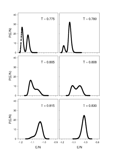
Figure 1: Energy per spin probability distributions (normalized histograms) for $\delta=2$ and $L=56$.

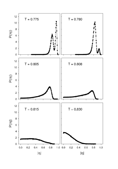
Figure 2: Orientational order parameter probability distributions (normalized histograms) for $\delta=2$ and $L=56$.

The presence of pairs of peaks in both the energy per spin and the orientational order parameter distributions, located at three distinct ranges of values, is a clear signature of the existence of three different phases, with two phase transitions between them. The low energy peak is associated with a peak in the order parameter centered around $\left|\eta\right|\approx 1$, thus corresponding to a phase with long range orientational order. Moreover, an analysis of a stripe order parameter introduced below (and also a direct inspection of the typical spin configurations at those energies) shows that this is an ordered striped phase with $h=2$. The highest energy peak is associated with a peak in the order parameter centered at $\eta=0$. A direct inspection of the associated typical spin configurations at those energies shows indeed that they correspond to a tetragonal liquid phase. On the other hand, the intermediate energy phase is associated with a peak of the order parameter centered around $\left|\eta\right|\approx 0.81$, thus corresponding to a state with broken $90^{o}$ rotational symmetry. In Fig.3a we illustrate a typical spin configuration in this intermediate phase for $L=64$ and $T=0.78$. We see that this phase is characterized by a high density of topological defects, mainly dislocations in the directions of the underlying striped structure. The same type of defects have been observed in Fe on Cu ultrathin films near the phase transition (see Fig.2 in Ref.Vaterlaus et al. (2000)). Such defects reduce the average value of the orientational order parameter and their presence is in agreement with the qualitative description of the Ising nematic phase introduced by Abanov and coauthors Abanov et al. (1995). To confirm this assumption we calculated the spatial correlations along the coordinate directions given by

$$C_{x}(r) \equiv \frac{1}{N}\sum_{y}\sum_{x}\left<\sigma_{x,y}\;\sigma_{x+r,y}\right>$$ (3)

$$C_{y}(r) \equiv \frac{1}{N}\sum_{y}\sum_{x}\left<\sigma_{x,y}\;\sigma_{x,y+r}\right>$$ (4)

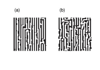
Figure 3: Typical spin configurations in the nematic phases for $\delta=2$ and $L=64$. (a) $T=0.78$, the orientational order parameter for this configuration is $|\eta|\approx 0.8$; (b) $T=0.807$ and $|\eta|\approx 0.59$

An example of the behavior of $C_{x}(r)$ and $C_{y}(r)$ in the intermediate phase is shown in Fig.4 for $L=92$ and $T=0.78$. This figure shows clearly that the correlations decay algebraically in one of the coordinate directions and exponentially in the other.We see that the intermediate phase is characterized by long range orientational order but does no t present positional order. Although the description level of the elastic approximation of Abanov and coauthors does not allow a simple derivation of the spin-spin spatial correlations, the above features are in qualitative agreement with their characterization of the nematic phase.

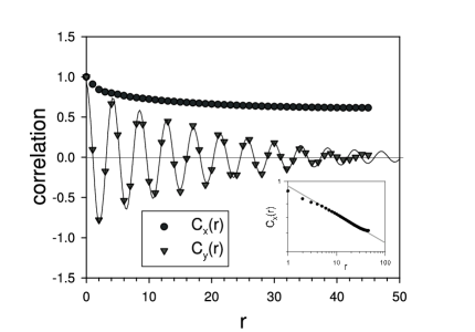
Figure 4: Spatial correlation functions along the coordinate directions in a nematic phase for $\delta=2$, $T=0.78$ and $L=92$. The continuous line corresponds to a fitting using a function $f(r)=A\exp{(r/\xi)\,\sin{(k_{0}\,r+\phi)}}$, with fitting parameters $k_{0}=1.47$, $\xi=17.4$ and $\phi=1.63$. Notice that $k_{0}\approx\pi/2$, the wave vector of the striped structure with $h=2$ (ground state for $\delta=2$). The log-log plot of $C_{x}$ in the inset shows that it decays at large distances with a power law $r^{-\omega}$, with an exponent $\omega\approx 0.12$.

To further characterize the different phases we defined a stripe order parameter through the static structure factor

$$S(\vec{k})\equiv\left<\left|\hat{\sigma}_{\vec{k}}\right|^{2}\right>=\frac{1}{N^{2}}\sum_{\vec{r}}\sum_{\vec{r}\,^{\prime}}C(\vec{r},\vec{r}\,^{\prime})e^{i\vec{k}.(\vec{r}-\vec{r}\,^{\prime})}$$ (5)

where $\hat{\sigma}_{\vec{k}}=\frac{1}{N}\sum_{\vec{r}}e^{i\vec{k}\vec{r}}\sigma_{\vec{r}}$ is the discrete Fourier transform of $\sigma_{\vec{r}}$. It can be shown that in a pure striped state of width $h$ the only non-zero components correspond to $(k_{x},k_{y})=(0,\pm\pi p/h)$ (horizontal stripes) or $(k_{x},k_{y})=(\pm\pi p/h,0)$ (vertical stripes), where $p$ takes all the odd integer values between one and $h$. For instance, in a pure $h=2$ vertical striped state it can be shown that

$$S(\vec{k})=\frac{1}{2}\;\delta_{k_{y},0}\;\left(\delta_{k_{x},\pi/2}+\delta_{k_{x},-\pi/2}\right)$$ (6)

Now, since all the phases we are dealing with in this case present a discrete rotational symmetry, either of $90^{o}$ or $180^{o}$ respect to the coordinate axes, the maxima of $S(\vec{k})$ will be located at $(k_{x},k_{y})=(\pm k_{0},0)$ and/or $(k_{x},k_{y})=(0,\pm k_{0})$, with $k_{0}$ some value close to $\pi/2$. Then we can define the stripe order parameter as

$$\eta_{s}=2\left(S(k_{0},0)+S(0,k_{0})\right)$$ (7)

(this definition can be easily generalized to consider underlying ground states of arbitrary width $h$). This order parameter will take values close to one for states with long range $h=2$ stripe order and zero (in the thermodynamic limit) for any state without long range positional order. For instance, let us consider a system in which correlations decay exponentially in the $x$ direction and remain almost constant in the $y$ direction, namely, $C(\vec{r},\vec{r}\,^{\prime})=\exp{(-\lambda|x-x^{\prime}|)}\;\cos{(k_{0}\,x)}$; this is a rough approximation of the behavior we observe in Fig.4, where the algebraic decay in one of the coordinate directions is extremely slow. Substituting into the definition of $S(\vec{k})$ and replacing the sums by integrals, in the large $L$ limit we get

$$S(\vec{k}) \sim \frac{\delta_{k_{y},0}}{L}\int_{0}^{\infty}e^{-\lambda\,x}cos(k_{0}\,x)\cos{k_{x}\,x}\;dx$$

$$\sim \frac{\delta_{k_{y},0}}{2L}\left(\frac{\lambda}{(k_{x}-k_{0})^{2}+\lambda^{2}}+\frac{\lambda}{(k_{x}+k_{0})^{2}+\lambda^{2}}\right)$$ (8)

If the correlation length $\xi_{s}=\lambda^{-1}$ is independent of the system size we have that the stripe order parameter goes to zero as $\eta_{s}\sim L^{-1}$ when $L\rightarrow\infty$. In a tetragonal liquid state we can assume for the correlation the following form

$$C(\vec{r},\vec{r}\,^{\prime})=e^{-\lambda(|x-x^{\prime}|+|y-y^{\prime}|)}\;cos(k_{0}\,|x-x^{\prime}|)\;cos(k_{0}\,|y-y^{\prime}|)$$ (9)

which possesses the tetragonal symmetry. We have then

$$S(\vec{k}) \sim \frac{1}{4L^{2}}\left(\frac{\lambda}{(k_{x}-k_{0})^{2}+\lambda^{2}}+\frac{\lambda}{(k_{x}+k_{0})^{2}+\lambda^{2}}\right.$$

$$+ \left.\frac{\lambda}{(k_{y}-k_{0})^{2}+\lambda^{2}}+\frac{\lambda}{(k_{y}+k_{0})^{2}+\lambda^{2}}\right)$$ (10)

which reproduces the observed crown shape of the structure factor observed in a tetragonal liquid state, both in numerical simulationsDe’Bell et al. (2000) and in Fe/Cu films imagesPortmann et al. (2003). In this case we have that the stripe order parameter goes to zero as $\eta_{s}\sim L^{-2}$ when $L\rightarrow\infty$.

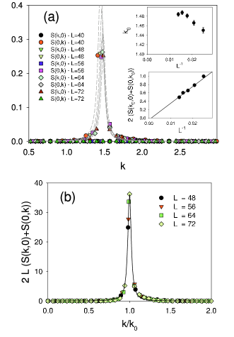
Figure 5: (a) Static structure factors $S(k,0)$ and $S(0,k)$ at $T=0.78$ for different system sizes. The dashed lines correspond to Lorentzian fittings $f(k)=\lambda/((k-k_{0})^{2}+\lambda^{2})$. The upper inset shows the fitted parameter $k_{0}$ vs. $L^{-1}$. The lower inset shows that the maximum of $S(\vec{k})$ scales as $L^{-1}$. (b) $2\;L(S(k,0)+S(0,k))$ vs $k/k_{0}$ for the same numerical data in (a); the continuous line is a Lorentzian fitting. The data collapse of the different curves shows that the whole curve $S(\vec{k})$ scales as $L^{-1}$, as predicted by Eq.(8).

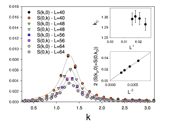
Figure 6: Static structure factors $S(k,0)$ and $S(0,k)$ at $T=0.95$ for different system sizes. The continuous lines correspond to Lorentzian fittings $f(k)=\lambda/((k-k_{0})^{2}+\lambda^{2})$. The upper inset shows the fitted parameter $k_{0}$ vs. $L^{-1}$. The lower inset shows that the maximum of $S(\vec{k})$ scales as $L^{-2}$. It can be also shown that the whole curve $S(\vec{k})$ scales as $L^{-2}$, as predicted by Eq.(10).

We performed numerical calculations of the structure factor in the three different phases for different system sizes up to $L=72$. First we calculated it in the low energy phase by letting the system to equilibrate from a vertical $h=2$ ground state configuration at $T=0.77$, just below the estimated transition temperature between the low and the intermediate energy phases $T_{1}\approx 0.772$ (see next section). We found that $S(\vec{k})=c\;\delta_{k_{y},0}\;(\delta_{k_{x},\pi/2}+\delta_{k_{x},-\pi/2})$, where $c$ quickly converges to a value $c\approx 0.48$ consistently with Eq.(6), thus confirming the long range stripe character of the low energy phase. Next we let the system to equilibrate in the intermediate phase at $T=0.78$. In Fig.5a we plot $S(k,0)$ and $S(0,k)$ for different system sizes. We observe that, while one of the two functions remains almost zero for all $k$, the other presents two symmetric peaks at $k=\pm k_{0}$ (only one is shown in the figure) which are very well fitted by a Lorentz function, in agreement with Eq.(8). We see that $k_{0}$ saturates into a value $k_{0}\approx 1.48$ while the maxima (or equivalently the order parameter $\eta_{s}$) goes to zero as $L^{-1}$. Moreover, the data collapse of the curves for different values of $L$ when $2\;L(S(k,0)+S(0,k))$ is plotted vs $k/k_{0}$ (see Fig.5b) shows that the whole curves scale as $L^{-1}$ in agreement with Eq.(8); this confirms that correlation length does not depend on $L$ in the thermodynamic limit and that the intermediate phase does not present LRO, thus confirming its nematic character. Finally, in Fig.6 we show $S(k,0)$ and $S(0,k)$ for different system sizes after equilibration in the tetragonal liquid at $T=0.95$. We see that both functions present two symmetric peaks at $k=\pm k_{0}$ (only those at $k>0$ are shown in the figure) which are very well fitted by Lorentz functions and that the maxima scale as $L^{-2}$, in excellent agreement with Eq.(10). Hence, we see that the stripe order parameter allows, not only to distinguish long range orientational order, but also discriminate between the tetragonal and the nematic phases through its finite size scaling.

It is worth mentioning that the two-peak structure in $P(E)$ and $P(\eta)$ associated with the nematic-tetragonal phase transition can only be appreciated in both type of histograms only for system sizes $L\geq 40$. For system sizes $L<40$ the two peaks are so close to each other that the phase transition cannot longer be resolved. In that situation the tetragonal and the nematic structures are almost indistinguishable, the latter appearing as a slightly elongated tetragonal oneCannas et al. (2004). While this strong finite size effect disappears for system sizes $L\geq 40$, there still remain similar finite size effects associated with the nematic-tetragonal phase transition up to system sizes $L=64$. This can be seen in Fig.7, where we show the histograms for the energy and the order parameter for $L=64$ and different temperatures around that transition. If we look at the energy per spin histogram (Fig.7a) we just see that the high energy peak becomes skewed towards the right and broadens around $T=0.81$ (compare with Fig.1). However, when looking at the orientational order parameter histogram (Fig.7b) we see that the single peak observed for smaller system sizes (see Fig.2) at that temperature range splits for $L=64$ into two distinct peaks, one centered at $|\eta|\approx 0.8$ and the other at $|\eta|\approx 0.6$. In Fig.3b we can see an example of a typical spin configuration in the second case. We see that the system still exhibits nematic order, the main difference with the configuration of Fig.3a being a higher density of domain walls perpendicular to the underlying striped structure (disclinations), which reduce the value of $|\eta|$. These results suggest the existence of different nematic phases separated by first order phase transitions between them. However, to verify this assumption much larger system sizes would be required.

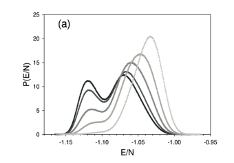
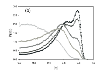
Figure 7: Histograms for $\delta=2$ and $L=64$, for temperatures around the nematic-tetragonal transition. (a) Energy per spin; temperatures from left to right: $T=0.804$, $0.805$, $0.807$, $0.810$ and $0.815$. (b) Orientational order parameter; same temperatures as in (a), but from right to left.

Next, we considered the case $\delta=1$, for which the ground state corresponds to a striped state with $h=1$ and the transition temperature is located aroundGleiser et al. (2002) $T=0.4$. In Fig.8 we show the typical structure of the histograms for the energy and the order parameter observed for system sizes up to $L=48$. While we do not see in this case a double peak structure in the energy per spin histogram (Fig.8a) as in the $\delta=2$ case, the broadening of the energy histogram around $T=0.4$ and its skewed form at both sides of the transition, together with a slight double peak structure of the orientational parameter (although difficult to see, the numerical data in Fig.8b show the presence of a minimum for $T=0.401$ between $\eta=0$ and $|\eta|\approx 0.6$) suggest a single first order phase transition. Moreover, a direct inspection of the typical spin configuration associated with the different distributions indicate a direct phase transition from the striped to the tetragonal phase, without any trace of an intermediate nematic state (notice that the location of the maximum of $P(|\eta|)$ moves continuously towards one below the transition point). This scenario will be confirmed by a direct thermodynamical analysis in the next section. However, based in the previously observed finite size effects for $\delta=2$, the possible existence of a nematic phase in a narrow range of temperatures for much larger system sizes cannot be excluded.

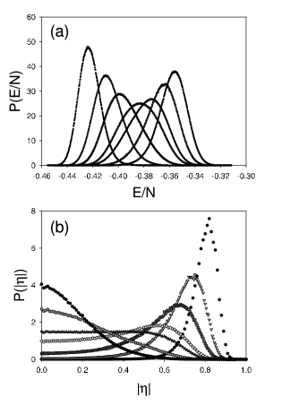
Figure 8: Histograms for $\delta=1$ and $L=48$.(a) Energy per spin; temperatures from left to right: $T=0.380$, $0.390$, $0.395$, $0.399$, $0.401$, $0.405$and $0.410$. (b) Orientational order parameter; same temperatures as in (a), but from right to left.

III Phase transitions

We now turn our attention to the stripe-nematic and nematic-tetragonal phase transitions in the $\delta=2$ case. To characterize them we analyzed the finite size scaling behavior of the moments of the energy, namely, the specific heat and the fourth order cumulant

$$C(L,T)=\frac{1}{NT^{2}}\left(\left<H^{2}\right>-\left<H\right>^{2}\right)$$ (11)

$$V(L,T)=1-\frac{\left<H^{4}\right>}{3\left<H^{2}\right>^{2}}$$ (12)

To check the simulations results we also calculated the average energy per spin $u(T)\equiv-\left<H\right>/N$ and compared its derivative with respect to temperature with Eq.(11); both results coincide within the numerical error. We also analyzed the average of the absolute value of the orientational order parameter $\left<\left|\eta\right|\right>$ and the associated susceptibility

$$\chi_{\eta}(L,T)=\frac{N}{T}\left(\left<\eta^{2}\right>-\left<\left|\eta\right|\right>^{2}\right)$$ (13)

All these quantities were obtained from the corresponding histograms for system sizes up to $L=64$. In Fig.9 we show the behavior of the energy moments and in Fig.10 of the average order parameter and its associated susceptibility (the results for $L=64$ are not shown for clarity).

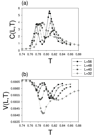
Figure 9: Moments of the energy for $\delta=2$ and different system sizes . (a) Specific heat Eq.(11); (b) Fourth order cumulant Eq.(12).

We see that the specific heat shows two distinctive maxima at size-dependent pseudo–critical temperatures $T_{1}^{c}(L)<T_{2}^{c}(L)$, while the fourth order cumulant shows two distinctive minima at pseudo–critical temperatures $T_{1}^{v}(L)<T_{2}^{v}(L)$, associated with the stripe-nematic and the nematic-tetragonal transitions respectively (notice that both the maximum at $T_{2}^{c}$ and the minimum at $T_{2}^{v}$ are almost unperceptive for $L=32$). On the other hand, the orientational order parameter shows jumps in behavior at each transition, but the associated susceptibility only shows a clear size dependent maximum at a size–dependent pseudo–critical temperature $T_{2}^{\chi}(L)$, corresponding to the nematic–tetragonal transition. This is consistent with the fact the $90^{o}$ rotational symmetry is broken at this phase transition. Although a second peak seems to emerge at lower temperatures for the largest size considered, it is very small and much more larger system sizes would be required to asses the presence of a size dependent peak associated with the stripe-nematic transition. From Fig.11 we see that the pseudo–critical temperatures of the specific heat and the fourth order cumulant scale as $T_{1}^{v}(L)\sim T_{1}+A_{1}/L^{2}$, $T_{1}^{c}(L)\sim T_{1}+B_{1}/L^{2}$, $T_{2}^{v}(L)\sim T_{2}+A_{2}/L^{2}$, $T_{2}^{c}(L)\sim T_{2}+B_{2}/L^{2}$, with $A_{1}>B_{1}$ and $A_{2}>B_{2}$. This is the expected scaling behavior at first order phase transitions Challa et al. (1986); Lee and Kosterlitz (1991). The extrapolation to $L\rightarrow\infty$ gives the values $T_{1}=0.772\pm 0.002$ and $T_{2}=0.797\pm 0.005$ showing that, although narrow, there is a well resolved range of temperatures in which the nematic phase exists in the thermodynamic limit. Moreover, from Fig.12 we also see that $T_{2}^{\chi}(L)\sim T_{2}+C/L^{2}$, where the extrapolation to $L\rightarrow\infty$ gives the same value for $T_{2}$ as the previous calculation. This behavior is also consistent with a first order phase transitionLee and Kosterlitz (1991).

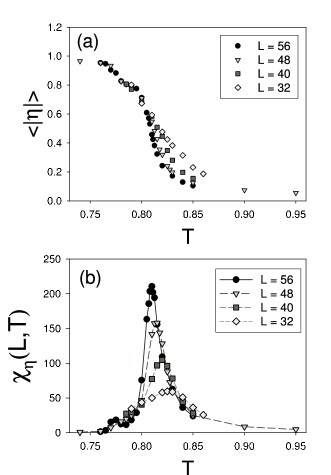
Figure 10: Moments of the orientational order parameter Eq.(2) for $\delta=2$ and different system sizes. (a) Average of the absolute value; (b) Associated susceptibility Eq.(13).

However, when looking at Fig.9 a clear difference in finite size scaling of the maxima of the specific heat and the minima of the fourth order cumulant between both transitions appears: while the minimum of $V$ at $T_{2}^{v}$ rapidly saturates at a constant value when $L\rightarrow\infty$, the minimum of $V$ at $T_{1}^{v}$ shows scaling behavior, approaching systematically to $2/3$. From Fig.13 we see that the maximum of the specific heat at $T_{2}^{c}$ increases as $L^{2}$ for system sizes up to $L=56$, as expected in a first order transition, but it shows a little departure from this behavior for $L=64$. However, such departure is probably due to systematic errors introduced by the presence of two phase transitions (see section II) that cannot be resolved for small system sizes. The scaling of $\chi_{\eta}(T_{2}^{\chi})$ is similar to that of $C(T_{2}^{2})$. On the other hand, the maximum of $C$ at $T_{1}^{c}$ saturates clearly in a finite value when the system size increases. It can also be shown that $2/3-V(T_{1}^{v})\sim L^{-2}$. This behavior can be understood if we look at the energy per spin histogram at the temperature where both maxima have the same height. If we call $e_{str}(L)$ and $e_{nem}(L)$ the energies per spin at which those maxima occur, in a first order phase transition it is expected that they will scale asLee and Kosterlitz (1991) $e_{str}(L)-u_{str}\sim L^{-1}$ and $e_{nem}(L)-u_{nem}\sim L^{-1}$, $u_{str}$ and $u_{nem}$ being the specific internal energies of both phases (the striped and the nematic ones, in this case) in the thermodynamic limit. Then, the maximum of the specific heat is expected to scale in a two-dimensional system asLee and Kosterlitz (1991) $C(T_{1}^{c})\sim L^{2}\,\left(e_{nem}(L)-e_{str}(L)\right)^{2}$, while $2/3-V(T_{1}^{v})\sim\left(e_{nem}(L)-e_{str}(L)\right)^{2}+{\cal O}(L^{-2})$. In Fig.14 we see that $e_{str}(L)$ and $e_{nem}(L)$ show the expected scaling, but they converge to the same value, so that $e_{nem}(L)-e_{str}(L)\sim L^{-1}$ and this explains the observed behaviors of the maximum of $C$ and the minimum of $V$. This shows that the internal energy at the stripe-nematic transition becomes continuous in the thermodynamic limit. However, a thermodynamical singularity still develops in that limit. This can be seen by looking at the scaling of the free energy barrier between both phases, which can be calculated asLee and Kosterlitz (1991)

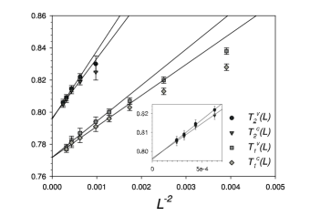
Figure 11: Finite size scaling of the pseudo-critical temperatures for the maxima of the specific heat ($T_{1}^{c}$ and $T_{2}^{c}$) and the minima of the fourth order cumulant ($T_{1}^{v}$ and $T_{2}^{v}$) for $\delta=2$ and system sizes up to $L=64$. The inset shows a zoom of the same curves around $T_{2}$.

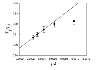
Figure 12: Finite size scaling of the pseudo-critical temperatures for the maxima of the susceptibility for $\delta=2$ and system sizes up to $L=64$.

$$\Delta F=\ln{\left(\frac{P_{max}}{P_{min}}\right)}$$ (14)

where $P_{max}\equiv P(e_{nem})=P(e_{str})$ is the value of the common maximum of energy per spin histogram and $P_{min}$ is the value of the minimum between them. In Fig.15 we see that $\Delta F\sim L$ in both phase transitions, which is the expected scaling in a first order phase transitionLee and Kosterlitz (1991). In particular, in the case of the stripe-nematic transition it means that, even when both states acquire the same energy, there is a divergent free energy barrier between them. Finally, we analyzed the difference between the values of the parameter $\eta$ at which the maxima in the corresponding histogram occur in the stripe-nematic phase transition $\Delta\eta(L)=\eta_{str}-\eta_{nem}$. A finite size scaling analysis similar to the previous ones shows that $\Delta\eta(L)\sim\Delta\eta(\infty)+D/L^{2}$, with $\Delta\eta(\infty)=0.075\pm 0.01$. Hence, a finite jump in this parameter, even small, persists in the thermodynamic limit, consistently with the discontinuous jump in the stripe order parameter already observed in the previous section.

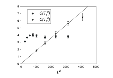
Figure 13: Finite size scaling of the maxima of the specific heat at $T_{1}^{c}$ and $T_{2}^{c}$ for $\delta=2$ and system sizes up to $L=64$.

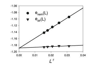
Figure 14: Finite size scaling of the energies per spin at which both maxima in the corresponding probability distribution occur, for the stripe–nematic phase transition for $\delta=2$ and system sizes up to $L=64$; for every value of $L$ the temperature is chosen such that $P(e_{nem})=P(e_{str})$

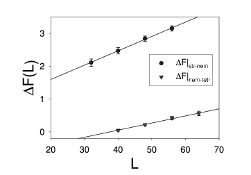
Figure 15: Finite size scaling of the free energy barrier Eq.(14) between phases in the stripe–nematic and the nematic–tetragonal phase transitions for $\delta=2$.

A specific heat peak saturation has been observed numerically in different systems exhibiting a KT type phase transition, such as the 2D XY modelGupta and Baillie (1992) and generalizations and the 1D Ising model with $1/r^{2}$ ferromagnetic interactionsLuijten and Messingfeld (2001); Imbrie and Newman (1988). This last model is particularly interesting, since it presents long range order in the low temperature phase (at variance with the XY models, which present only short range order) and the order parameter (magnetization) is discontinuous at the transitionAinzenman et al. (1988), in an analogous way to the model we are considering here. However, an important difference should be noted: in the above mentioned examples of the KT transition the extrapolation of the pseudo critical temperature at which the maximum of the specific heat is located appears slightly above the critical temperature.

Next we considered the tetragonal-stripe phase transition in the case $\delta=1$. As we have seen in section II, the equilibrium histograms suggest a weak first order phase transition. Since a finite size scaling approach would require system sizes much larger than the allowed by the present computational capabilities, to confirm the supposed first order nature of the transition we considered another type of approach.

Since we know the value of the ground state energy $u_{g}$ and also the asymptotic infinite temperature internal energy, we can obtain the free energy for different temperatures integrating the measured internal energies. We checked that the internal energy is independent of system size for $48\leq L\leq 64$, and we chose a $N=48\times 48$ lattice in order to measure internal energy. The equilibrium internal energy as a function of temperature for the stripe and tetragonal phases are shown in Fig.(16). Using this energy curve we fit the stripe energy by a polynomial function $u_{str}(T)=u_{g}+a_{1}T^{a_{2}}+a_{3}T^{a_{4}}+a_{5}T^{a_{6}}$ and the tetragonal energy with a sum of hyperbolic functions $u_{tetr}(T)=b_{0}\textrm{tanh}(\frac{b_{1}}{T})+b_{2}\textrm{tanh}(\frac{b_{3}}{T})$, whose parameters are shown in the caption. By means of the thermodynamical relation:

$$\beta f(\beta)=\beta_{0}f_{0}(\beta_{0})+\int_{\beta_{0}}^{\beta}u(\beta)d\beta,$$ (15)

where $\beta=1/T$ and $\beta_{0}=1/T_{0}$, we obtained the free energy per particle, $f(\beta)$ for the striped and tetragonal phases (shown in Fig. (17)). The transition temperature is obtained by imposing $f_{str}(T)=f_{tetr}(T)$, which gives $T_{m}=0.404$. The entropy is obtained directly by the thermodynamical relation $s=-\frac{df}{dT}$ and the result is shown in the Fig.(18). A weak first order transition is apparent, in agreement with the behavior of the energy and order parameter histograms of Fig.8.

These results for the thermodynamic functions point to a unique phase transition for $\delta=1$, from a high temperature tetragonal liquid phase to a low temperature striped phase. There is no trace of a third Ising nematic phase as for $\delta=2$, at least for $48\leq L\leq 64$ system sizes.

This conclusion is natural in this case where the equilibrium low temperature phase corresponds to stripes of width $h=1$. Once defects begin to emerge due to thermal fluctuations, disclinations appear naturally and the orientational order will rapidly decay , at variance with the expected behavior for wider stripes which will be more stable to the appearance of topological defects.

Figure 16: Internal energy per spin $u$ versus $T$ for $\delta=1$ and $N=48\times 48$. Also shown best fits to the low temperature stripe and high temperature tetragonal regions, as described in the text. The best fit parameters for $u_{str}$ are $a_{1}=1952.54;a_{2}=10.8491;a_{3}=10.8441;a_{4}=5.73016;a_{5}=-58.0638$ and $a_{6}=7.34061$, and for $u_{tetr}$ are $b_{0}=-1.47926;b_{1}=0.0817682;b_{2}=0.0559538$ and $b_{3}=-3.05417$. The ground state energy is $u_{g}=-0.4677$.

Figure 17: Free energy per spin $f$ versus $T$ for $\delta=1$. The stripe and tetragonal free energies cross each other around $T_{m}=0.404$. The functions obtained from equation (15) are $f_{str}=u_{g}+\frac{a_{1}}{1-a_{2}}T^{a_{2}}+\frac{a_{3}}{1-a_{4}}T^{a_{4}}+\frac{a_{5}}{1-a_{6}}T^{a_{6}}$ and $f_{tetr}=\frac{b_{0}}{b_{1}}T\textrm{ln}(\textrm{cosh}\frac{b_{1}}{T})+\frac{b_{2}}{b_{3}}T\textrm{ln}(\textrm{cosh}\frac{b_{3}}{T})-T\textrm{ln}(2)$, where $\beta_{0}=0$ for the tetragonal and $\beta_{0}=\infty$ for the striped phase.

Figure 18: Entropy per spin $s$ versus $T$ for $\delta=1$. The slight discontinuity at the transition temperature is consequence of a weak first order phase transition.

IV Metastability

The presence of diverging free energy barriers between the different phases found in the previous section for $\delta=2$ lead us to consider the possible existence of dynamical metastable (i.e., quasi–stationary) states. To this end, we performed cooling and heating numerical calculations according to the following protocol. We first let the system equilibrate at a temperature high enough to ensure that it is in the tetragonal liquid phase. We then cooled the system at a fixed cooling rate $r$, that is, the temperature was decreased as $T(t)=T_{0}-r\;t$, where $T_{0}$ is the initial temperature and the time $t$ is measured in MCS. The temperature was reduced in every MC run down to a value well below the range associated with the different phase transitions, while recording at different points the energy and the orientational order parameter $|\eta|$ of the system. Every curve was then averaged over different initial conditions and different sequences of the random noise. For every system size we calculated those curves for decreasing cooling rates until they became independent of the cooling rate. In this way we simulated a process of quasi-static cooling. Once we obtained the quasi-static cooling curves we performed a quasi-static heating from zero temperature up to high temperatures, starting from the ground state and using the same protocol and the same rate $r$.

In fig.19 we see an example of the quasi-static cooling-heating curves obtained for $L=48$ with a cooling rate $r=10^{-6}$; the results are compared with the equilibrium curves obtained in the previous section. Similar results were obtained for system sizes up to $L=64$. We do not observe super cooled tetragonal liquid states below $T_{2}$, but this is probably due to the relatively small values of the associated free energy barriers for the system sizes here considered. On the other hand, we observe a strong metastability associated with the stripe–nematic phase transition, which is consistent with the observed large free energy barriers. In particular, we see that the supercooled nematic state is observed down to temperatures well below $T_{1}$. To verify the quasi-equilibrium nature of the metastable nematic states, we calculated the two-times autocorrelation function

$$C(t_{1},t_{2})\equiv\frac{1}{N}\sum_{i}\;\left<S_{i}(t_{1})\,S_{i}(t_{2})\right>$$ (16)

after a quasi–static cooling to different temperatures $T<T_{1}$, down to $T=0.5$, for different pairs of values $t_{1}<t_{2}$. In all the cases we found that $C(t_{1},t_{2})$ depends only on the difference $t_{2}-t_{1}$ (as expected for a quasi–stationary process), for time scales up to $t=10^{6}$ MCS. For larger time scales the nematic phase finally decay into the striped one, apparently through a nucleation process. These results are not shown here, but a complete description of those calculations will be published shortlyCaS .

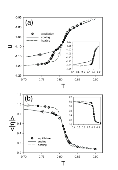
Figure 19: Cooling-heating curves for $\delta=2$, $L=48$ and $r=10^{-6}$. The insets show the same curves for a wider range of temperatures. (a) Average energy per spin (b) Average of the absolute value of the orientational order parameter.

V Discussion

The main contribution of this paper are the several evidences of the existence of nematic phases in an ultrathin magnetic film model, at least for some range of values of the exchange to dipolar intensities ratio. These results are in agreement with one of the two possible scenarios of the critical behavior of those systems predicted by the continuum approximation of Abanov and co–workersAbanov et al. (1995). Let us discuss first the stripe-nematic phase transition. Although the finite size scaling behavior of different quantities around that transition agree with that expected in a first order transition, both the fact that the energy becomes continuous and the saturation of the specific heat maximum in the thermodynamic limit are unusual in a simple first order transition, suggesting a more complex phenomenology. In fact, those properties strongly resemble those observed in the $1/r^{2}$ one dimensional Ising model transition point, namely, continuous energy, discontinuous order parameter and saturation of the specific heat maximum. These analogies suggest that some KT type mechanism, probably associated with the unbinding of dislocations, could be responsible of the observed phenomenology, in agreement with Abanov and coworkers prediction. The observed first-order-like finite size scaling behavior appears to be related with the discontinuous change of the orientational order parameter at the transition point in the thermodynamic limit, which suggests the existence of a finite density of dislocation pairs. Indeed, we observed the presence of an increasing number of dislocations pairs (bridges) in the striped phase at $T=T_{1}$ but, up to $L=72$ system sizes we didn’t find any evidence of QLRO (algebraic decaying correlations). One important consequence of such first-order-like phenomenology is the existence of diverging free energy barriers at that point, which has an important physical implication, namely, the possibility to obtain highly stable supercooled nematic states through cooling. This opens the possibility of having complex slow dynamical behaviors after a sudden quench, such as those observed in supercooled molecular liquids. We are investigating this problems and the results will be presented in a forthcoming publicationCaS .

Concerning the nematic-tetragonal phase transition, our results suggest a much more complex behavior than the expected from Abanov et al. results, who conjectured a second order phase transition. Although our results are inconclusive due to the presence of strong finite size effects, they suggest a complex phase diagram with multiple nematic phases, separated by first order transition lines, similar to that encountered by Grousson et alGrousson et al. (2001) in a related model, the 3D Coulomb frustrated Ising ferromagnet. However, the departure from the expected first order finite size scaling observed for $L=64$ in the maximum of the specific heat (see Fig.13) and the susceptibility, could be an indication of a behavior similar to that observed in the stripe-nematic transition. Hence, the possibility of a nematic-tetragonal KT phase transition, associated with a disclination unbinding mechanism, cannot be excluded. A similar scenario appears in a related problem, namely, the two-dimensional meltingStrandburg (1988). On the other hand, the Hartree approximation of the Landau-Ginzburg version of the present model predicts a fluctuation induced first order phase transitionCannas et al. (2004) for any value of $\delta$.

The case of small exchange/dipolar ratio is simpler in the sense that only one transition is observed from a stripe phase directly to a tetragonal liquid phase. We obtained evidence that this transition is a weak first order one.

Although we have analyzed the critical behavior of this system for relatively small values of the exchange/dipolar ratio ($\delta=1$ and $\delta=2$), the present results may help to understand the critical behavior for larger values. Booth and coworkersBooth et al. (1995) analyzed the behavior of the specific heat and the orientational order parameter for $\delta=3$ and $\delta=4.45$ and system sizes up to $L=64$. While their results suggest a continuous stripe-tetragonal phase transition, numerical results based on time series analysis from Casartelli and coworkersCasartelli et al. (2004), for the same parameters and system sizes, indicate that the transition is first order. For those values of $\delta$ the stable low temperature phase is composed by stripes with a larger width ($h=4$), so much more larger system sizes would be required to allow the appearance of a large density of topological defects (dislocations and disclinations of the stripes). Therefore, for larger system sizes one could expect a scenario similar to that observed for $\delta=2$, namely, the appearance of nematic order in a narrow range of temperatures.

The experimental verification of the different transitions and phases suggested by theory and simulations is an important challenge which can be reached in the near future due to the emergence of new observation techniques.

Fruitful discussions with A. Cavagna and T. Grigera are acknowledged. We thank very useful suggestions and comments from anonymous referees. This work was partially supported by grants from CONICET (Argentina), Agencia Córdoba Ciencia (Argentina), SeCyT, Universidad Nacional de Córdoba (Argentina), CNPq (Brazil) and ICTP grant NET-61 (Italy).

References

- Allenspach et al. (1990) R. Allenspach, M. Stampanoni, and A. Bischof, Phys. Rev. Lett. 65, 3344 (1990).
- Vaterlaus et al. (2000) A. Vaterlaus, C. Stamm, U. Maier, M. G. Pini, P. Politi, and D. Pescia, Phys. Rev. Lett. 84, 2247 (2000).
- De’Bell et al. (2000) K. De’Bell, A. B. MacIsaac, and J. P. Whitehead, Rev. Mod. Phys. 72, 225 (2000).
- Politi (1998) P. Politi, Comments Cond. Matter Phys. 18, 191 (1998).
- Booth et al. (1995) I. Booth, A. B. MacIsaac, J. P. Whitehead, and K. De’Bell, Phys. Rev. Lett. 75, 950 (1995).
- Abanov et al. (1995) A. Abanov, V. Kalatsky, V. L. Pokrovsky, and W. M. Saslow, Phys. Rev. B 51, 1023 (1995).
- Sampaio, deAlbuquerque, and deMenezes (1996) L. C. Sampaio M. P. deAlbuquerque and F. S. deMenezes, Phys. Rev. B 54, 6465 (1996).
- Stoycheva and Singer (2000) A. D. Stoycheva and S. J. Singer, Phys. Rev. Lett. 84, 4657 (2000).
- Toloza et al. (1998) J. H. Toloza, F. A. Tamarit, and S. A. Cannas, Phys. Rev. B 58, R8885 (1998).
- Stariolo and Cannas (1999) D. A. Stariolo and S. A. Cannas, Phys. Rev. B 60, 3013 (1999).
- Gleiser et al. (2002) P. M. Gleiser, F. A. Tamarit, and S. A. Cannas, Physica D 168-169, 73 (2002).
- Gleiser et al. (2003) P. M. Gleiser, F. A. Tamarit, S. A. Cannas, and M. A. Montemurro, Phys. Rev. B 68, 134401 (2003).
- Cannas et al. (2004) S. A. Cannas, D. A. Stariolo, and F. A. Tamarit, Phys. Rev. B 69, 092409 (2004).
- Casartelli et al. (2004) M. Casartelli, L. Dall’Asta, E. Rastelli, and S. Regina, J. Phys. A: Math. Gen. 37, 11731 (2004).
- Portmann et al. (2003) O. Portmann, A. Vaterlaus, and D. Pescia, Nature 422, 701 (2003).
- Wu et al. (2004) Y. Z. Wu, C. Won, A. Scholl, A. Doran, H. W. Zhao, X. F. Jin, and Z. Q. Qiu, Phys. Rev. Lett. 93, 117205 (2004).
- Portmann et al. (2006) O. Portmann, A. Vaterlaus, and D. Pescia, Phys. Rev. Lett. 96, 047212 (2006).
- (18) It is worth noting that the definition of the Hamiltonian in ReferencesDe’Bell et al. (2000); MacIsaac et al. (1995); Booth et al. (1995) is slightly different from ours. While in those papers the dipolar term contains a sum over all pairs of spins, here we consider the sum over every pair of spins just once. This leads to the equivalence , being the exchange parameter in the above references. Since the dipolar parameter also fixes the energy units in our work, there is also a factor between the critical temperatures obtained in those works and ours.
- MacIsaac et al. (1995) A. B. MacIsaac, J. P. Whitehead, M. C. Robinson, and K. De’Bell, Phys. Rev. B 51, 16033 (1995).
- Challa et al. (1986) M. S. S. Challa, D. P. Landau, and K. Binder, Phys. Rev. B 34, 1841 (1986).
- Lee and Kosterlitz (1991) J. Lee and J. M. Kosterlitz, Phys. Rev. B 43, 3265 (1991).
- Gupta and Baillie (1992) R. Gupta and C. F. Baillie, Phys. Rev. B 45, 2883 (1992).
- Luijten and Messingfeld (2001) E. Luijten and H. Messingfeld, Phys. Rev. Lett. 86, 5305 (2001).
- Imbrie and Newman (1988) J. Z. Imbrie and C. M. Newman, Commun. Math. Phys. 118, 303 (1988).
- Ainzenman et al. (1988) M. Ainzenman, J. T. Chayes, L. Chayes, and C. M. Newman, J. Stat. Phys. 50, 1 (1988).
- (26) S. A. Cannas, D. A. Stariolo and F. A. Tamarit, to be published.
- Grousson et al. (2001) M. Grousson, G. Tarjus, and P. Viot, Phys. Rev. E 64, 036109 (2001).
- Strandburg (1988) K. J. Strandburg, Rev. Mod. Phys 60, 161 (1988).