Spectral signatures of Holstein polarons

1 Fundamentals

1.1 Self-trapping phenomenon

Electrons or holes delocalised in a perfect rigid lattice can be “trapped” in a potential well produced by displacements of atoms if the particle-lattice interaction is sufficiently strong [1]. Such trapping is energetically favoured over wide-band Bloch states if the carrier’s binding energy exceeds the strain energy required to produce the trap. Since the potential itself depends on the carrier state, this highly non-linear process is called “self-trapping” (Fig. 1). A self-trapped state is referred to as “large” if it extends over multiple lattice sites. Alternatively, for a quasi-particle (QP) with extremely large effective mass $m^{*}$ – practically confined to a single site – the state is designated as “small”. Self-trapping does not imply a breaking of translational invariance, i.e., in a crystal these eigenstates are still itinerant allowing, in principle, for coherent transport with an extremely small bandwidth.

Figure 1: Polaron formation: The standard phase transition concept fails to describe this highly non-linear feedback phenomenon.

Introducing the concept of polarons into physics, the possibility of electron self-trapping was pointed out by Landau as early as 1933 [2]. Self-trapped polarons consisting of electrons accompanied by phonon clouds can be found, e.g., in alkali(ne) metal (earth) halides, II-IV- and group-IV semiconductors, and organic molecular crystals [3]. With the observation of polaronic effects in high-$T_{c}$ cuprates [4] and colossal magneto-resistance manganites [5], research on polarons has attracted renewed attention (see also [6]).

1.2 Holstein model

Depending on the relative importance of long- and short-range electron-lattice interaction, simplified models of the Fröhlich [7] or Holstein [8] type have been widely used to analyse polaronic effects in solids with displaceable atoms. The spinless Holstein Hamiltonian reads

$$H=-t\sum_{\langle i,j\rangle}c_{i}^{\dagger}c_{j}-\sqrt{\varepsilon_{p}\omega_{0}}\sum_{i}(b_{i}^{\dagger}+b_{i})n_{i}+\omega_{0}\sum_{i}b_{i}^{\dagger}b_{i}\,.$$ (1)

Here $c_{i}^{[\dagger]}$ and $b_{i}^{[\dagger]}$ are the annihilation [creation] operators of a (spinless) fermion and a phonon at Wannier site $i$, respectively, and $n_{i}=c_{i}^{\dagger}c_{i}$. In (1), the following idealisations of real electron-phonon (EP) systems are made: (i) the electron transfer $t$ is restricted to nearest-neighbour pairs $\langle ij\rangle$; (ii) the charge carriers are locally coupled to a dispersionless optical phonon mode [$\varepsilon_{p}$ measures the polaron binding energy and $\omega_{0}$ is the bare phonon frequency ($\hbar=1$)]; (iii) the phonons are treated within the harmonic approximation.

Nevertheless, as yet, none of the various analytical treatments, based on weak- and strong-coupling adiabatic and anti-adiabatic perturbation expansions [9], are suited to investigate the physically most interesting polaron transition region. In the latter, the characteristic electronic and phononic energy scales are not well separated and non-adiabatic effects become increasingly important, implying a breakdown of the standard Migdal approximation. Quasi-approximation-free numerical methods like quantum Monte Carlo (QMC) [10, 11, 12], exact diagonalisation (ED) [13], or the density matrix renormalisation group (DMRG) [14] can, in principle, close the gap between the weak- and strong-EP-coupling limits, therefore representing the currently most reliable tools to study polarons close to the cross-over regime (see also [15]).

1.3 Ground-state properties

Previous numerical work mainly focused on the single-polaron problem. There are two control parameters common in use, the first being the adiabaticity ratio $\omega_{0}/t$. In the adiabatic limit $\omega_{0}/t\to 0$, the motion of the particle is affected by quasi-static lattice deformations, whereas in the opposite anti-adiabatic limit $\omega_{0}/t\to\infty$, the lattice deformation adjusts instantaneously to the carrier position. The second parameter is the EP coupling strength $\lambda=\varepsilon_{p}/2\mathrm{D}t$, the ratio of the polaron binding energy of an electron confined to a single site and the free electron half-bandwidth in D dimensions.

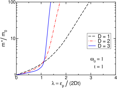
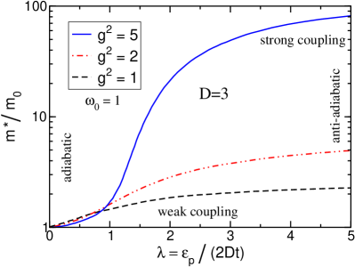
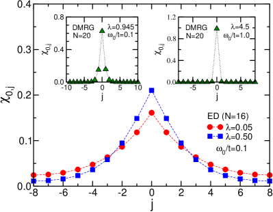
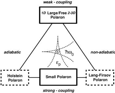
Figure 2: Effective mass $m^{*}/m_{0}$ (data taken from [16]), (normalised) electron-phonon correlation function $\chi_{0,j}=\langle n_{0}(b^{\dagger}_{0+j}+b_{0+j})\rangle/2g\langle n_{0}\rangle$, and schematic “phase diagram” of the Holstein model. Depending on the adiabaticity of the system, the cross-over regime is determined by the more stringent of the two conditions $\lambda\simeq 1$ and $g\simeq 1$. Thus starting from “light” ($\omega_{0}/t<1$) or “heavy” ($\omega_{0}/t>1$) electrons it is possible to understand the formation of small adiabatic “Holstein” or anti-adiabatic “Lang-Firsov” polarons as two limiting cases of a general picture.

Figure 2 summarises selected ground-state characteristics of small-polaron formation, showing results obtained by (variational) ED [16, 17] and DMRG [14]. The transition to a polaron with large effective mass takes place at $\lambda\simeq 1$, and is much sharper in higher dimensions [16]. Adiabatic theory predicts an energy barrier separating quasi-free (infinite radius) polarons from small-sized lattice polarons in $\mathrm{D}>1$, but not in $\mathrm{D}=1$. However, the (variational) ED data show that for $\omega_{0}>0$, the cross-over is continuous in any dimension, i.e., the Holstein model does not exhibit a true phase transition [16, 17], in accordance with the theorem of Gerlach and Löwen [18]. In the anti-adiabatic regime, a further parameter ratio, $g^{2}=\varepsilon_{p}/\omega_{0}$, turns out to be crucial. Small-polaron formation takes place if both $\lambda>1$ and $g^{2}>1$. Note that the mass enhancement notably deviates from the strong-coupling (perturbation theory) result $\exp(g^{2})$ at intermediate phonon frequencies [16]. The cross-over from an only weakly phonon-dressed electron to a small polaron also shows up very clearly in the correlation between electron- and phonon-displacements (not be equated with the polaron radius): At the critical coupling, there is a strong enhancement of the on-site correlations [17, 14]. Furthermore, $\chi_{0,j}/\chi_{0,0}$ decays more rapidly as D increases, i.e., the surrounding phonons are localised closer to the electron in higher dimensions [16].

The ground-state properties discussed so far constitute only one aspect of polaron physics. Of equal importance is the dynamical response of a polaronic system to external perturbations. For a moving (small) polaron there is a perpetual exchange of momentum between the electron and the deformation field [19]. Photoemission spectroscopy and inelastic neutron scattering should therefore be able to detect the strong interrelation of electron and phonon degrees of freedom. The strong mixing of purely electronic states with lattice vibrational excitations should be visible in the optical response as well. In the following sections, we therefore present exact numerical results for electron/phonon spectral functions and the optical conductivity in the framework of the Holstein model. A very efficient Chebyshev-expansion-based algorithm for the calculation of such dynamical correlation functions is outlined in [15] (for more details see [20]).

2 Photoemission spectra

Examining the dynamical properties of polarons, it is of particular interest whether a QP-like excitation exists in the spectrum. This is probed by direct (inverse) photoemission, where a bare electron is removed (added) from (to) the many-particle system. The intensities (transition amplitudes) of these processes are determined by the imaginary part of the retarded one-particle Green’s functions,

$$G^{\pm}(k,\omega)=\langle\langle c_{k}^{\mp};c_{k}^{\pm}\rangle\rangle_{\omega}=\lim_{\eta\to 0^{+}}\ \langle\psi_{0}|c_{k}^{\mp}\,[\omega+\mathrm{i}\eta\mp H]^{-1}\,c_{k}^{\pm}|\psi_{0}\rangle\,,$$ (2)

i.e., by the wave-vector resolved spectral functions

$$A^{\pm}(k,\omega)=-\frac{1}{\pi}\mathrm{Im}\,G^{\pm}(k,\omega)=\sum_{m}|\langle\psi_{m}^{\pm}|c_{k}^{\pm}|\psi_{0}\rangle|^{2}\,\delta[\,\omega\mp(E_{m}^{\pm}-E_{0})]$$ (3)

with $c_{k}^{+}=c_{k}^{\dagger}$ and $c_{k}^{-}=c_{k}$. These functions test both the excitation energies $E_{m}^{\pm}-E_{0}$ and the overlap of the ground state $|\psi_{0}\rangle$ with the exact eigenstates $|\psi_{m}^{\pm}\rangle$ of a $(N_{\rm e}\pm 1)$-particle system. Hence, $G^{+}(k,\omega)$ [$G^{-}(k,\omega)$] describes the propagation of an additional electron [a hole] with momentum $k$ [$-k$] and energy $\omega$. The electron spectral function of the single-particle Holstein model corresponds to $N_{\rm e}=0$, i.e., $A^{-}(k,\omega)\equiv 0$. $A(k,\omega)=A^{+}(k,\omega)+A^{-}(k,\omega)$ can be determined, e.g., by cluster perturbation theory (CPT) [21, 15]: We first calculate the Green’s function $G^{c}_{ij}(\omega)$ of a $N_{c}$-site cluster with open boundary conditions for $i,j=1,\dots,N_{c}$, and then recover the infinite lattice by pasting identical copies of this cluster along the edges, treating the inter-cluster hopping in first-order perturbation theory.

Figure 3 shows that at weak coupling (left panel), the electronic spectrum is nearly unaffected for energies below the phonon emission threshold. Hence, for the case considered here with $\omega_{0}$ lying inside the bare electron bandwidth $4Dt$, the renormalised dispersion $E(k)$ follows the tight-binding cosine dispersion (lowered $\propto\varepsilon_{p}$) up to some $k_{X}$, where the dispersionless phonon intersects the bare electron band. For $k>k_{X}$, electron and phonon states “hybridise”, and repel each other, leading to the well-known band-flattening phenomenon [22]. The high-energy incoherent part of the spectrum is broadened $\propto\varepsilon_{p}$, with the $k$-dependent maximum again following the bare cosine dispersion.

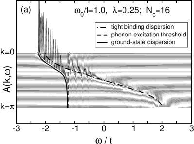
Figure 3: Spectral function of the 1D Holstein polaron calculated within CPT in the weak (a) and strong (b) non-adiabatic EP coupling regime. CPT is based on ED of a finite cluster with $N_{c}$ sites, $M=7$ ($\lambda=0.25$) and $M=25$ ($\lambda=2$) phonon quanta.

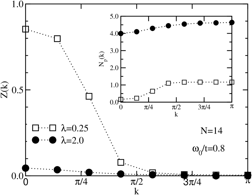
Figure 4: QP residue $Z(k)$ and mean phonon number $N_{\rm p}(k)$ (inset) obtained by ED at the allowed $k$ vectors of a 1D 14-site lattice with periodic boundary conditions. Note that $g^{2}$ roughly gives the mean phonon number in the strong-coupling case.

To substantiate this interpretation, we compute the QP weight and mean phonon number,

$$Z(k)=|\langle\psi^{+}_{k}|c^{\dagger}_{k}|\psi_{0}\rangle|^{2}\qquad\mbox{and}\qquad N_{\rm p}(k)=\sum_{i}\langle\psi^{+}_{k}|(b_{i}^{\dagger}+b_{i})|\psi_{0}\rangle\,,$$ (4)

for each $k$-sector (see Fig. 4). The $k$-dependent $Z$-factor can be taken as a measure of the “electronic contribution” to the QP. For weak EP coupling, we have $Z(k\ll k_{X})\lesssim 1$ [$Z(k>k_{X})\ll 1$], reflecting the electronic [phononic] character of the states at the band centre [band edge], which are basically zero-phonon [one-phonon] states (see Fig. 4, inset). Increasing the EP coupling, a strong mixing of electron and phonon degrees of freedom takes place, whereby – forming a small polaron – both quantum objects cease to exist independently. As expected, this leads to a significant suppression of the (electronic) QP residue $Z(k)$ for all $k$. Now the states $|\psi_{0}\rangle$, $|\psi_{k}^{\pm}\rangle$ are multi-phonon states, and the polaronic QP is heavy because it has to drag with it a large number of phonons in its phonon cloud (cf. Fig. 4, inset).

The inverse photoemission spectrum in the strong-coupling case is shown in the right panel of Fig. 3. First, we observe all signatures of the famous polaronic band-collapse, where a well-separated, narrow (i.e., strongly renormalised), coherent QP band is formed at $\omega\simeq-\varepsilon_{p}$. If we had calculated the polaronic instead of the electronic spectral function (3), nearly all spectral weight would reside in the coherent part, i.e., in the small-polaron band [23]. In contrast, $Z(k)$, defined by (4), is extremely small and approaches the strong-coupling result $Z=\exp(-g^{2})$ for $\lambda\,,g^{2}\gg 1$. Note that the inverse effective mass $m^{*}/m_{0}$ and $Z(k)$ differ if the self-energy is strongly $k$-dependent. This discrepancy has its maximum in the intermediate-coupling regime for 1D systems, but vanishes in the limit $\lambda\to\infty$ and, in any case, for $D=\infty$ [16]. The incoherent part of the spectrum is split into several sub-bands separated in energy by $\omega_{0}$, corresponding to excitations of an electron and one or more phonons (Fig. 3).

Finally, let us emphasise that for all couplings, the lowest-lying band in $A(k,\omega)$ almost perfectly coincides with the coherent polaron band-structure (solid line in Fig. 3) obtained by variational ED [16]. This method has been shown to give very accurate results for the infinite system, also underlining the high precision of our CPT approach.

3 Phonon spectra

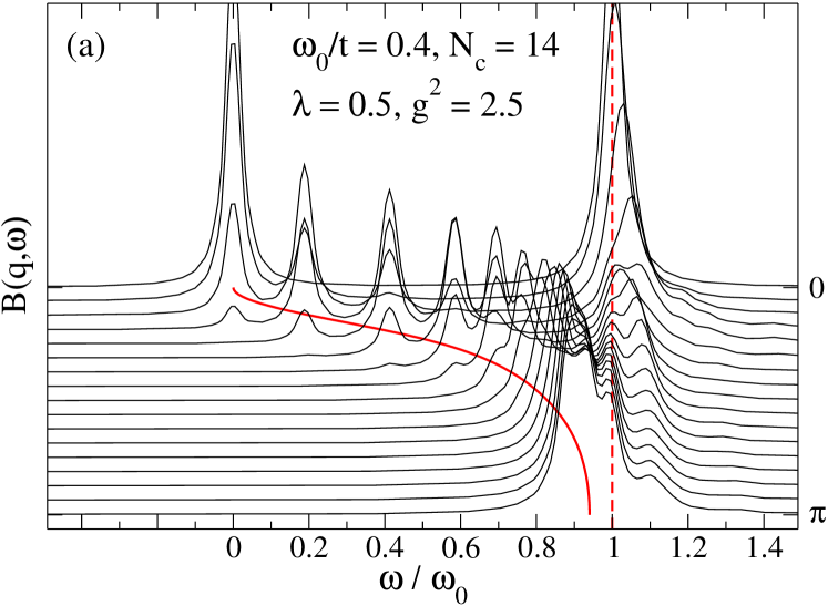
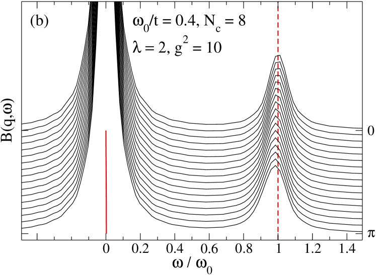
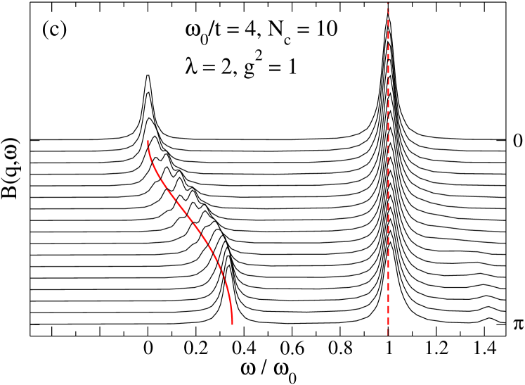
Figure 5: Phonon spectral function for the 1D single-electron Holstein model. The bare phonon frequency is indicated by a dashed vertical line. The solid line corresponds to the polaron band dispersion $E(k)-E(0)$, calculated using the method presented in [16]. Shown are exemplary results for the adiabatic weak and strong-EP-coupling [(a) and (b)] and anti-adiabatic intermediate-coupling [panel (c)] regimes.

Next we show that the phonon spectra provide additional useful information concerning the polaron dynamics. For this purpose, we calculate the $T=0$ spectral function $B(q,\omega)$, which is related to the phonon Green’s function $D(q,\omega)$ for $\omega>0$ by

$$B(q,\omega)=-\frac{1}{\pi}\mathrm{Im}\,D(q,\omega)\,,\quad D(q,\omega)=2\omega_{0}\langle\langle x_{q};x_{-q}\rangle\rangle_{\omega}\,,$$ (5)

where $x_{q}=N^{-\mbox{\small$\frac{1}{2}$}}\sum_{j}x_{j}\mbox{e}^{-{\rm i}jq}$ and $x_{j}=(b^{\dagger}_{j}+b_{j})/\sqrt{2\omega_{0}}$. Again we employ a cluster approach, determining first the cluster phonon Green’s function $D_{ij}^{c}(\omega)$, and afterwards, as in CPT, constructing the energy and momentum dependent Green’s function of the infinite lattice from $D(q,\omega)=\frac{1}{N_{c}}\sum_{i,j=1}^{N_{c}}D^{c}_{ij}(\omega)\text{ e}^{-{\rm i}q(i-j)}$. Since for the Holstein model the bare phonon Green’s function $D^{0}(\omega)=2\omega_{0}/(\omega^{2}-\omega_{0}^{2})$ is $k$-independent, this cluster expansion is identical to replacing the full real-space Green’s function $D_{ij}$ by $D^{c}_{ij}$.

Figures 5(a) and (b) show the evolution of the phonon spectrum with increasing EP interaction in the adiabatic case ($\omega_{0}/t=0.4$). For $\lambda=0.5$, there is a dispersive low-energy absorption reflecting the polaron band dispersion, as demonstrated by the comparison with variational-ED data for $E(k)$. If the weakly renormalised electron band intersects the (dispersionless) bare phonon excitation at some $q_{Y}$, level repulsion occurs and we observe two adjacent absorption features. At larger EP couplings, the polaron band separates completely from the bare phonon signature until, in the extreme strong-coupling limit, two almost flat absorption bands emerge, corresponding to the lowest (small) polaron band and the first excited band, separated by a one-phonon excitation. Both signals are strong because of the large “phonon content” in these states.

As stated above, in the anti-adiabatic regime, the small-polaron cross-over is determined by the ratio $g^{2}$, and occurs at about $g^{2}=1$. For $g^{2}\ll 1$, nearly the whole spectral weight resides in the bare phonon peak (if $\omega_{0}>4Dt$). The phonon spectrum near the transition point is shown in Fig. 5(c) for $\omega_{0}/t=4$. We detect a clear signature of the small-polaron band with renormalised width $W\simeq 1.5t$ – a factor of about ten larger than in the adiabatic case ($\lambda=1$, $\omega_{0}/t=0.4$; note that the excitation energy in Fig. 5 is plotted in units of $\omega_{0}$). The dispersionless excitation at $\omega_{0}$ is obtained by adding one phonon with momentum $q$ to the $k=0$ ground state. Above this pronounced peak, we find an “image” of the lowest polaron band – shifted by $\omega_{0}$ – with extremely small spectral weight, hardly resolved in Fig. 5.

4 Optical response

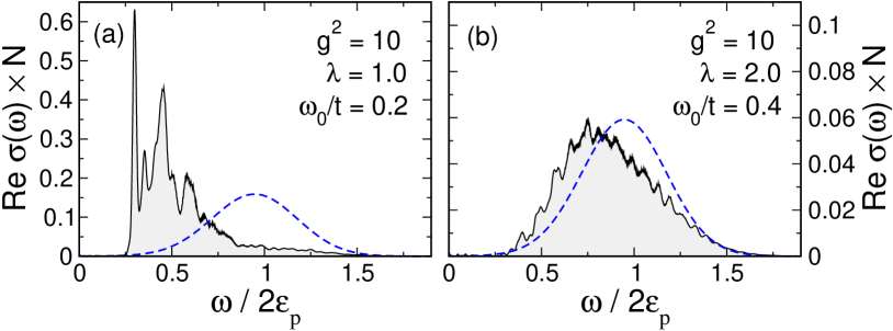
Figure 6: Optical conductivity (in units of $\pi e^{2}t^{2}$) of the 1D Holstein polaron at $T=0$ compared to the analytical small-polaron result (dashed line). ED data are for a system with $N=6$ sites and 45 phonons; $\sigma_{0}$ is determined to give the same integrated spectral weight as $\mbox{Re}\,\sigma(\omega>0)$.

We apply the ED-KPM scheme outlined in [15, 20, 24] to calculate the optical absorption of the 1D Holstein polaron. The results for the (regular) real part of the conductivity,

$$\mbox{Re}\,\sigma(\omega)=\frac{\pi}{\omega N}\sum_{E_{m}>E_{0}}|\langle\psi_{m}|\hat{\jmath}|\psi_{0}\rangle|^{2}\ \delta[\omega-(E_{m}-E_{0})]$$ (6)

(here $\hat{\jmath}=-\mbox{i}et\sum_{i}(c_{i}^{\dagger}c_{i+1}-c_{i+1}^{\dagger}c_{i})$ is the current operator), and possible deviations from established polaron theory are important for relating theory to experiment. The standard description of small polaron transport [25] yields for the $T=0$ ac conductivity

$$\mbox{Re}\,\sigma(\omega)=\frac{\sigma_{0}}{\sqrt{\varepsilon_{p}\omega_{0}}}\frac{1}{\omega}\exp\left[-\frac{(\omega-2\varepsilon_{p})^{2}}{4\varepsilon_{p}\omega_{0}}\right]\,.$$ (7)

For sufficiently strong coupling this formula predicts a weakly asymmetric Gaussian absorption peak centred at twice the polaron binding energy.

Figure 6 shows $\mbox{Re}\,\sigma(\omega)$ when polaron formation sets in (a), and above the transition point (b). For $\lambda=2$ and $\omega_{0}/t=0.4$, i.e., at rather large EP coupling but not in the extreme small-polaron limit, we find a pronounced maximum in the low-temperature optical response, which, however, is located somewhat below $2\varepsilon_{p}=2g^{2}\omega_{0}$, the value for small polarons at $T=0$. At the same time, the line-shape is more asymmetric than in small-polaron theory, with a weaker decay at the high-energy side, fitting even better to experiments on standard polaronic materials such as TiO₂ [26]. At smaller couplings, significant deviations from a Gaussian-like absorption are found, i.e., polaron motion is not adequately described as hopping of a self-trapped carrier almost localised on a single lattice site.

5 Many-polaron problem

Finally, we address the important issue how the character of the QPs of the system changes with carrier density. While for very strong EP coupling no significant changes are expected due to the existence of rather independent small (self-trapped) polarons with negligible residual interaction, a density-driven cross-over from a state with large polarons to a metal with weakly dressed electrons may occur in the intermediate-coupling regime [11]. This problem has recently been investigated experimentally by optical measurements on La_2/3(Sr/Ca)_1/3MnO_3 films [27].

In the Holstein model, the above-mentioned density-driven transition from large polarons to weakly EP-dressed electrons is expected to be possible only in 1D, where large polarons exist at weak and intermediate coupling. The situation is different for Fröhlich-type models [7, 28, 29] with long-range EP interaction, in which large-polaron states exist even for strong coupling and in $\mathrm{D}>1$.

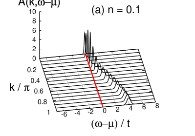
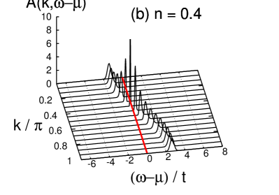
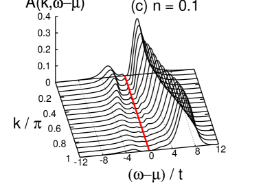
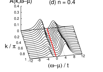
Figure 7: One-electron spectral function $A(k,\omega-\mu)$ of the 1D spinless Holstein model from QMC [11] for low ($n=0.1$) and high ($n=0.4$) carrier densities at weak [(a),(b); $\lambda=0.1$] and strong [(c),(d); $\lambda=2$] EP coupling, $\omega_{0}/t=0.4$, $N=32$, and $t/k_{\rm B}T=8$ (inverse temperature). Note that QMC cannot resolve features with very small spectral weight.

To set the stage, Fig. 7 shows the evolution of the one-electron spectral function $A(k,\omega-\mu)$ with increasing electron density $n$ in the weak- and strong-coupling limiting cases. In the former [Fig. 7(a),(b)], the spectra bear a close resemblance to the free-electron case for all $n$, i.e., there is a strongly dispersive band running from $-2t$ to $2t$, which can be attributed to weakly dressed electrons with an effective mass close to the non-interacting value. As expected, the height (width) of the peaks increases (decreases) significantly in the vicinity of the Fermi momentum, which is determined by the crossing of the band with the chemical potential $\mu$. In the opposite strong-coupling limit [Fig. 7(c),(d)], the spectrum exhibits an almost dispersionless coherent polaron band at $\mu$ (QMC, due to the use of maximum entropy, has problems resolving such extremely weak signatures). Besides, there are two incoherent features located above and below the chemical potential, broadened $\propto\varepsilon_{p}$, reflecting phonon-mediated transitions to high-energy electron states. At $n=0.4$, the photoemission spectrum for $k<\pi/2$ becomes almost symmetric to the inverse photoemission spectrum for $k>\pi/2$ and already reveals the gapped structure expected at $n=0.5$ due to the Peierls transition (charge-density-wave formation). The most important point, however, is the clear separation of the coherent band from the incoherent parts even at large $n$. This indicates that small polarons are well-defined QPs in the strong-coupling regime, even at high carrier density.

Figure 8 displays the inverse photoemission [$A^{+}(k,\omega)$] and photoemission spectra [$A^{-}(k,\omega)$] at intermediate EP coupling strength, determined by CPT at $T=0$.

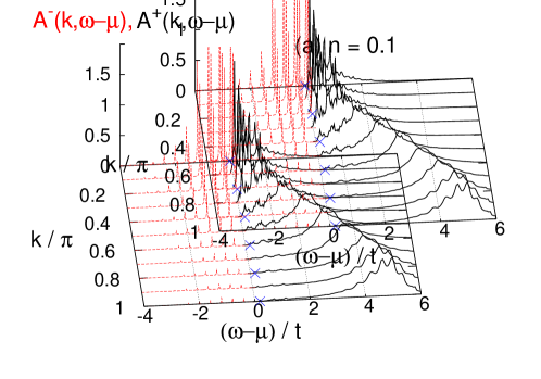
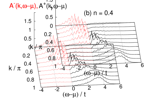
Figure 8: Single particle spectral functions $A^{-}(k,\omega)$ (red dashed lines) and $A^{+}(k,\omega)$ (black solid lines) for different band fillings $n$ at $\omega_{0}/t=0.4$ and $\lambda=1$ (CPT results with $N_{c}=10$). Blue crosses track the small-polaron band obtained by ED.

At $n=0.1$ we can also identify a (coherent) polaron band (blue crosses; cf. also the ED data in [11]). The Fermi energy $E_{\mathrm{F}}=\mu(T\to 0)$ is located within this signature. The large-polaron band has small electronic spectral weight especially away from $E_{\mathrm{F}}$ and flattens as an effect of the EP coupling at large $k$ (see Sec. 2). Below this band, there exist equally spaced phonon satellites, reflecting the Poisson distribution of phonons in the ground state. Above $E_{\mathrm{F}}$ there is a broad dispersive incoherent feature whose maximum follows closely the dispersion relation of free particles.

As $n$ increases, a well-separated coherent polaron band can no longer be identified. At about $n\simeq 0.3$ the deformation clouds of the (large) polarons start to overlap leading to a mutual (dynamical) interaction between the particles. Increasing the carrier density further, the polaronic QPs dissociate, stripping their phonon cloud. Now diffusive scattering of electrons and phonons seems to be the dominant interaction mechanism. As a result both, the phonon peaks in $A^{-}(k,\omega)$ and the incoherent part of $A^{+}(k,\omega)$ are washed out, the spectra broaden and ultimately merge into a single wide band [11, 30]. As can be seen from Fig. 8 (b), the incoherent excitations lie now arbitrarily close to the Fermi level. These are significant differences to the nearly free electron and small polaron spectra shown for the same carrier density in Figs. 7 (b) and (d), respectively. Obviously the low-energy physics of the system can no longer be described by small-polaron theory.

6 Summary and open problems

In this contribution, we have reviewed ground-state- and, most notably, spectral properties of Holstein polarons by means of quasi-exact numerical methods such as (variational) Lanczos diagonalisation, a kernel polynomial expansion technique, cluster perturbation theory, and quantum Monte Carlo. Our numerical approaches yield unbiased results in all parameter regimes, but are of particular value in the non-adiabatic intermediate-coupling regime, where perturbation theories and other analytical techniques fail. The data presented for the (inverse) photoemission, phonon- and optical spectra show that electron and phonon excitations become intimately, dynamically connected in the process of polaron formation.

Although we have now achieved a rather complete picture of the single (Holstein) polaron problem (perhaps dispersive phonons, longer-ranged EP interaction, finite temperature and disorder effects deserve closer attention), the situation is discontenting in the case of a finite carrier density. Here electron-phonon coupling competes with sometimes strong electronic correlations as in, e.g., unconventional 1D metals, quasi-1D MX chains, quasi-2D high-$T_{c}$ superconductors, 3D charge-ordered nickelates, or bulk colossal magneto-resistance manganites. The corresponding microscopic models contain (extended) Hubbard, Heisenberg or double-exchange terms, and maybe also a coupling to orbital degrees of freedom, so that they can hardly be solved even numerically with the same precision as the Holstein model. Consequently, the investigation of these materials and models will definitely be a great challenge for solid-state theory in the near future.

- [1] Firsov Y.A., Polarons (Izd. Nauka, Moscow), 1975; Rashba E.I., in Excitons, edited by E.I. Rashba and M.D. Sturge (North-Holland, Amsterdam), 1982, p. 543.
- [2] Landau L.D., Z. Phys., 3 (1933) 664.
- [3] Shluger A.L. and Stoneham A.M., J. Phys. Condens. Matter, 5 (1993) 3049.
- [4] Alexandrov A.S. and Mott N.F., Rep. Prog. Phys., 57 (1994) 1197.
- [5] Jaime M., Hardner H.T., Salamon M.B., Rubinstein M., Dorsey P. and Emin D., Phys. Rev. Lett., 78 (1997) 95;. Millis A.J., Nature, 392 (1998) 147.
- [6] Ranninger J., Proc. Int. School of Physics “Enrico Fermi”, Course CLXI, Polarons in Bulk Materials and Systems with Reduced Dimensionality, Eds. G. Iadonisi, J. Ranninger, G. de Filippis, (IOS Press, Amsterdam, Oxford, Tokio, Washington DC) 2006, pp 1-25.
- [7] Fröhlich H., Adv. Phys., 3 (1954) 325.
- [8] Holstein T., Ann. Phys. (N.Y.), 8 (1959) 325; 8 (1959) 343.
- [9] Migdal A.B., Sov. Phys. JETP, 7 (1958) 999; Lang I.G. and Firsov Y.A., Zh. Eksp. Teor. Fiz., 43 (1962) 1843; Marsiglio F., Physica C, 244 (1995) 21.
- [10] De Raedt H. and Lagendijk A., Phys. Rev. B, 27 (1983) 6097; Kornilovitch P.E., Phys. Rev. Lett., 81 (1998) 5382.
- [11] Hohenadler M., Neuber D., von der Linden W., Wellein G., Loos J. and Fehske H., Phys. Rev. B, (2005) 245111.
- [12] Mishchenko A. S., Proc. Int. School of Physics “Enrico Fermi”, Course CLXI, Polarons in Bulk Materials and Systems with Reduced Dimensionality, Eds. G. Iadonisi, J. Ranninger, G. de Filippis, (IOS Press, Amsterdam, Oxford, Tokio, Washington DC) 2006, pp 177-201.
- [13] Ranninger J. and Thibblin U., Phys. Rev. B, 45 (1992) 7730; Wellein G., Röder H. and Fehske H., Phys. Rev. B, 53 (1996) 9666.
- [14] C. Zhang, Jeckelmann E. and White S.R., Phys. Rev. Lett., 80 (1998) 2661; Jeckelmann E. and White S.R., Phys. Rev. B, 57 (1998) 6376.
- [15] Jeckelmann E. and Fehske. H., Proc. Int. School of Physics “Enrico Fermi”, Course CLXI, Polarons in Bulk Materials and Systems with Reduced Dimensionality, Eds. G. Iadonisi, J. Ranninger, G. de Filippis, (IOS Press, Amsterdam, Oxford, Tokio, Washington DC) 2006, pp 247-284.
- [16] Ku L.C., Trugman S.A. and Bonča J., Phys. Rev. B, 65 (2002) 174306; see also Bonča J., Trugman S.A. and Batistić I., Phys. Rev. B, 60 (1999) 1633.
- [17] Wellein G. and Fehske H., Phys. Rev. B, 58 (1998) 6208.
- [18] Gerlach B. and Löwen H., Rev. Mod. Phys., 63 (1991) 63.
- [19] Alexandrov A.S. and Ranninger J., Phys. Rev. B, 45 (1992) 13109.
- [20] Weiße A., Wellein G., Alvermann A. and Fehske H., Rev. Mod. Phys. 78 275 (2006).
- [21] Sénéchal D., Perez D. and Pioro-Ladrière M., Phys. Rev. Lett., 84 (2000) 522; Hohenadler M., Aichhorn M. and von der Linden W., Phys. Rev. B, 68 (2003) 184304.
- [22] Stephan W., Phys. Rev. B, 54 (1996) 8981; Wellein G. and Fehske H., Phys. Rev. B, 56 (1997) 4513.
- [23] Fehske H., Loos J. and Wellein G., Z. Phys. B, 104 (1997) 619; Loos J., Hohenadler M. and Fehske H., J. Phys.: Condens. Matter 18 (2006) 2453.
- [24] Schubert G., Wellein G., Weiße A., Alvermann A. and Fehske H., Phys. Rev. B, 72, (2005) 104304
- [25] Emin D., Phys. Rev. B, 48 (1993) 13691.
- [26] Kudinov E.K., Mirlin D.N. and Firsov Y.A., Fiz. Tverd. Tela, 11 (1969) 2789.
- [27] Hartinger C. et al., Phys. Rev. B, 69 (2004) 100403(R).
- [28] Alexandrov A.S. and Kornilovitch P.E., Phys. Rev. Lett., 82 (1999) 807; Fehske H., Loos J. and Wellein G., Phys. Rev. B, 61 (2000) 8016.
- [29] Devreese J.T. and Tempere J., Phys. Rev. B, 64 (2001) 104504.
- [30] Hohenadler M., Wellein G., Alvermann A. and Fehske H., Physica B 378-380 (2006) 64.