Classical wave experiments on chaotic scattering

Abstract

We review recent research on the transport properties of classical waves through chaotic systems with special emphasis on microwaves and sound waves. Inasmuch as these experiments use antennas or transducers to couple waves into or out of the systems, scattering theory has to be applied for a quantitative interpretation of the measurements. Most experiments concentrate on tests of predictions from random matrix theory and the random plane wave approximation. In all studied examples a quantitative agreement between experiment and theory is achieved. To this end it is necessary, however, to take absorption and imperfect coupling into account, concepts that were ignored in most previous theoretical investigations. Classical phase space signatures of scattering are being examined in a small number of experiments.

1 Introduction

Experiments with classical waves, originally conceived to study the spectral properties of closed systems, have more recently become an important tool to study the scattering properties of open systems as well.

At about 1980 the main experimental information on spectra and scattering properties of chaotic systems came from nuclear physics and resulted in the development of random matrix theory by Wigner, Dyson, Mehta and others on one side [1], and of scattering theory by Weidenmüller and coworkers on the other side [2].

Interest in the properties of chaotic systems suddenly renewed, when it was conjectured by Casati et al[3] and Bohigas et al[4] that the universal properties of all chaotic systems should be described by random matrix theory. An equivalent of the conjecture for open systems was formulated somewhat later by Blümel and Smilansky [5]. These conjectures proved to be extremely useful and gave a new impetus to the whole field.

The experimental situation, however, remained unsatisfactory until 1990, when the first analogue experiments were published, starting with vibrating solids [6] and chaotic microwave cavities [7]. Meanwhile the technique has been extended to water surface and pressure waves [8, 9] and optical systems [10, 11, 12]. At about the same time the tremendous progress in the fabrication of semiconductor microstructures allowed to study the transport properties of submicron size structures of various types such as quantum dots [13], tunnelling barriers [14], and quantum corrals [15]. The state of the art till 1999 can be found in chapter 2 of reference [16].

In the beginning these experiments focussed on the spectral properties of closed systems though there was already an early experiment looking for the scattering properties of an open microwave system [17]. Strictly speaking, the systems are always open, due to the necessity to introduce antennas or transducers to perform the measurements. Therefore scattering theory is mandatory for a quantitative interpretation of the measurements. This is why it became necessary to establish a relation between the Green’s function of the closed system and the scattering matrix [18], which is a direct equivalent of a corresponding expression derived in nuclear physics many years ago. For the case of an isolated resonance the well-known Breit-Wigner formula is recovered [19]. Details will be given in section 2. The same equivalence also holds for quantum-dot systems, as long as electron-electron interactions can be neglected. Thus with respect to scattering theory it does not make any difference whether atomic nuclei, quantum dots, microwave cavities, or vibrating blocks are involved, provided one is interested in the universal features only.

This allows experimental tests of theoretical predictions from scattering theory with an unprecedented precision. A number of important consequences of scattering theory have been demonstrated with classical waves, but never found in nuclei, such as the algebraic decay of the scattering matrix from a system with a small number of channels [20, 21], or the fact that with increasing coupling to the channels the resonances eventually become narrow again [22], known as resonance trapping.

There are a number of clear advantages of microwave resonators and vibrating blocks as compared e. g. to nuclei, but also to quantum dots. First of all, the geometry is perfectly known, and the coupling to the external channels can be calculated explicitly from the antenna geometry. The systems are clean, and if there are impurities, they are introduced intentionally. The geometry can easily be varied thus allowing level dynamic measurements of different types, which is impossible for nuclei, and can be achieved only in a very restricted way in quantum dots. Further advantages arise from the fact that the relevant wavelengths in microwave resonators or vibrating blocks are of the order of mm to cm resulting in very convenient system sizes. Last but not least the experiments can be performed at room temperature since there are no dephasing processes as in quantum dots which have to be frozen out. This advantage is lost in microwave experiments using superconducting cavities, but still the applied temperatures of some K are far above the 0.01 to 1 K temperatures usually applied in quantum dot experiments.

In this review we present results from microwave resonators, vibrating blocks, and optical systems, and their comparison with the predictions of scattering theory. Wave experiments on localization in disordered systems are excluded since they are treated in a separate contribution to this volume [23]. Results on quantum dots, tunneling diodes and other mesoscopic structures are excluded as well. They would have deserved a contribution of their own, and will be mentioned only in cases where a comparison with results from experiments with classical waves seems appropriate.

This review is organized as follows. In the next section a Green’s function technique is applied to establish a relation between the scattering matrix and the Green’s function of the system. In addition the random superposition of plane waves model is introduced to describe amplitude distributions in chaotic cavities. Though demonstrated for the example of a flat microwave cavity where there is a perfect analogy to quantum mechanics, the results of this section can be applied without changes to all experiments with classical waves. Therefore this section is the basis for all following ones where the results in open microwave cavities, vibrating blocks, and optical systems are presented.

2 The scattering matrix for billiard systems

2.1 The billiard Breit-Wigner formula

A microwave billiard is a special example for a scattering system, where the measuring antennas take the role of the scattering channels. We are now going to discuss the consequences of the external coupling for resonance positions and widths.

Let us start with a two-dimensional quantum billiard of arbitrary shape, and assume that there are a number of channels coupled to the billiard with diameters small compared to the wave length. Let $\psi(\bi{r},k)$ be the amplitude of the field within the billiard while matter waves enter and exit through the different channels. $\psi(\bi{r},k)$ obeys the Helmholtz equation

$$\left(\Delta+k^{2}\right)\psi=0\,.$$ (1)

Close to the channels the field is given by a superposition of incoming and outgoing circular waves,

$$\psi(\bi{r},k)=a_{i}H_{0}^{(1)}(k_{i}|\bi{r}-\bi{r_{i}}|)-b_{i}H_{0}^{(2)}(k_{i}|\bi{r}-\bi{r_{i}}|)\,,$$ (2)

where $\bi{r_{i}}$ is the position of the $i$th channel. $a_{i}$ and $b_{i}$ are the amplitudes of the waves entering and leaving the billiard through the channel, and $H_{0}^{(1)}(x)$ and $H_{0}^{(2)}(x)$ are Hankel functions. Denoting the amplitude vectors of the waves entering or leaving the billiard by $a=(a_{1},a_{2},\dots,a_{N})$ and $b=(b_{1},b_{2},\dots,b_{N})$, respectively, the scattering matrix for the billiard system is defined by the relation

$$b=Sa\,.$$ (3)

The $a_{i}$ and $b_{i}$ are obtained by matching fields and their normal derivatives at the coupling positions of the channels. This is achieved by means of Green’s function techniques. Details can be found, e. g., in Section 6.1.2 of Ref. [16]. Thus one obtains

$$S=\frac{1-\imath W^{\dagger}GW}{1+\imath W^{\dagger}GW}\,,$$ (4)

where the matrix elements $W_{nm}$ of $W$ contain the information of the coupling of the $n$th eigenfunction to the $m$th channel, and $G$ is given by

$$G=\frac{1}{k^{2}-H}\,,$$ (5)

where $H=-\Delta$ is the Hamilton operator for the undisturbed system.

An explicit calculation of the $W_{nm}$ has to take into account the details of the coupling geometries. For antennas in microwave resonators this has been achieved in Ref. [24]. But it is common practice to treat the $W_{nm}$ as free parameters which are taken from the experiment.

An elementary transformation of equation (4) yields the equivalent expression

$$S=1-2iW^{\dagger}\frac{1}{k^{2}-H+\imath WW^{\dagger}}W\,,$$ (6)

For the case of non-overlapping resonances and point-like coupling this reduces to

$$S_{ij}(k)=\delta_{ij}-2\imath\gamma\bar{G}(\bi{r_{i}},\bi{r_{j}},k)\,,$$ (7)

with the modified Green’s function

$$\bar{G}(\bi{r_{i}},\bi{r_{j}},k)=\sum_{n}\frac{\psi_{n}(\bi{r_{i}})\psi_{n}(\bi{r_{j}})}{k^{2}-k_{n}^{2}+\imath\gamma\sum_{k}\left|\psi_{n}(\bi{r_{k}})\right|^{2}}\,$$ (8)

(see reference [18]). $\psi_{n}$ are the real eigenfunctions of the closed systems and $\gamma$ describes the antenna coupling. The last equations constitute the billiard equivalent of the Breit-Wigner formula well-known from nuclear physics for many years [25]. Often the scattering matrix is studied on the time domain. To this end the Fourier transform is performed,

$$\hat{S}_{ij}(t)=\frac{1}{2\pi}\int S_{ij}(k)\rme^{-\imath\omega t}\,\rmd\omega\,,$$ (9)

where $\omega=\hbar k^{2}/2m$. It follows

$$\hat{S}_{ij}(t)=\delta_{ij}\,\delta(t)-\frac{\hbar\gamma}{m}\sum_{n}\psi_{n}(\bi{r_{i}})\psi_{n}(\bi{r_{j}})\exp{\left[-\left(\imath\omega_{n}+\frac{1}{2}\Gamma_{n}\right)t\right]}\,,$$ (10)

with $\Gamma_{n}=(\hbar\gamma/m)\sum_{k}\left|\psi_{n}(\bi{r_{k}})\right|^{2}$. This holds for the quantum mechanical case. For non-dispersive classical waves we have instead $\omega=ck$, and $\gamma$ has to be replaced by $k\gamma$ in Eqs. (7) and (8). Thus one obtains

$$\hat{S}_{ij}(t)=\delta_{ij}\,\delta(t)-2\gamma c\sum_{n}\psi_{n}(\bi{r_{i}})\psi_{n}(\bi{r_{j}})\sin\left(\omega_{n}t\right)\rme^{-\frac{1}{2}\Gamma_{n}t}\,,$$ (11)

where now $\Gamma_{n}=\gamma c\sum_{k}\left|\psi_{n}(\bi{r_{k}})\right|^{2}$. In both cases $\Gamma$ corresponds to the decay rate of the square of the field.

Equation (7) shows that the complete modified Green’s function $\bar{G}(\bi{r_{i}},\bi{r_{j}},k)$ can be obtained from a transmission measurement between two antennas of variable position [18]. A reflection measurement at one antenna only yields the spectrum and the modulus of the wave function [7, 26]. The ‘true’ wave function $G(\bi{r_{i}},\bi{r_{j}},k)$, however, is never obtained since the resonances are broadened by $\Gamma_{n}$. This is the price to be paid for every measurement.

2.2 The random plane wave approximation

A model which proved to be very useful to describe field distributions and correlation in chaotic billiards is the random plane wave approximation. It assumes that the wave function can be described at any point, not too close to the boundary, by a random superposition of plane waves, entering from different directions, but with the same modulus of the wave number,

$$\psi(\bi{r})=\sum\limits_{n}a(\bi{k_{n}})\rme^{\imath\bi{k_{n}}\bi{r}}\,,\qquad|\bi{k_{n}}|=k\,.$$ (12)

The model has been independently introduced in different fields, among others in acoustics [27] and in quantum mechanics of chaotic systems [28]. It is known as Berry’s conjecture in the quantum chaos community. The random plane wave approximation can be obtained from the Green’s function of the billiard by averaging over a small energy window as was shown by Hortikar, Srednicki [29] and further exploited by Urbina, Richter [30].

As an immediate consequence of the central limit theorem one obtains a Gaussian distribution for the amplitudes of the wave function of closed systems,

$$p(\psi)=\sqrt{\frac{A}{2\pi}}\exp\left(-\frac{A\psi^{2}}{2}\right)\,,$$ (13)

where $A$ is the billiard area (see e. g. Section 6.2 of Ref. [16]). In open systems real and imaginary part of $\psi(r)$ are uncorrelated and both Gaussian distributed.

The model allows the explicit calculation of various correlation functions, the most popular among them the spatial amplitude autocorrelation function

$$c_{\psi}(\bi{r_{1}},\bi{r_{2}}) = \langle\psi^{*}(\bi{r_{1}})\psi(\bi{r_{2}})\rangle$$ (14)

$$= \frac{1}{A}J_{0}(kr)\,,$$

where $r=\left|\bi{r_{1}}-\bi{r_{2}}\right|$.

The random plane wave approximation can be used to calculate the distribution of line widths. The line width in a billiard with $\nu$ attached channels is given by a sum over the squares of $\nu$ Gaussian distributed random numbers, (compare the expressions following equations (10) and (11)). The distribution $p_{\nu}(x)$ is hence a $\chi^{2}$ distribution

$$p_{\nu}(x)=\left(\frac{A}{2}\right)^{\nu/2}\frac{1}{\Gamma\left(\nu/2\right)}x^{\nu/2-1}\rme^{-\frac{A}{2}x}\,.$$ (15)

The distribution of resonance depths for a reflection measurement can be obtained as well. According to equation (8) the resonance depths are proportional to $\left|\psi_{n}(\bi{r})\right|^{2}$, where $\bi{r}$ is the antenna position. The depth distribution function for a closed system is thus a $\chi^{2}$ distribution with $\nu=1$,

$$p_{1}(x)=\sqrt{\frac{A}{2\pi x}}\rme^{-\frac{A}{2}x}\,,$$ (16)

i. e. a Porter-Thomas distribution. For an completely open system one obtains a $\chi^{2}$ depth distribution with $\nu=2$, which is just a single exponential,

$$p_{2}(x)=\frac{A}{2}\rme^{-\frac{A}{2}x}\,.$$ (17)

The model allows the calculation of averages of transients of various correlations of scattering matrix elements as well. From equation (10) we obtain for the average of $|\hat{S}_{ij}(t)|^{2}$

$$\hat{C}_{ij}(t)=\langle|\hat{S}_{ij}(t)|^{2}\rangle\sim\left(1+\frac{4\gamma t}{\hbar A}\right)^{-(2+\nu/2)}\,,$$ (18)

i. e. an algebraic decay is expected with an exponent reflecting the number of attached channels. For a very large number of channels the $\chi^{2}$ distribution concentrates in a narrow peak, which is again a consequence of the central limit theorem. In this limit there is a cross-over in the decay of $\hat{C}_{ij}(t)$ to a single exponential behaviour, as is immediately evident from equation (10),

$$\hat{C}_{ij}(t)\sim\rme^{-\Gamma t}\,.$$ (19)

It follows that the Fourier transform of $\hat{C}_{ij}(t)$, which due the the convolution theorem of Fourier theory is just the energy autocorrelation function of the respective scattering matrix elements, is described by a Lorentzian. This is the regime of the Ericson fluctuations [31], well-known in nuclear physics for many years. It is noteworthy that the same universal fluctuation statistics were long ago noted in acoustics as well [32, 33].

2.3 Acoustic and elastodynamic systems

The expressions (1) to (19) of the previous subsections have direct analogs in acoustic and elastodynamic systems. The concepts of ray propagation, and the more abstract formalisms, are essentially identical. The differences are chiefly in the governing wave equation (1) and in the details of experimental transduction.

Like microwaves in 2-d billiards, waves in 2-d shallow water tanks [34, 27] are governed by equation (1), with $k^{2}$ interpreted as $\omega^{2}/gh$ ($g$: acceleration of gravity, $h$: water depth). Chinnery [9] presents acoustic measurements in a deep water tank in quasi-2-d cylindrical geometries. These experiments differ from the corresponding 2-d microwave experiments in that they generally have non-Dirichlet boundary conditions at tank edges and lower $Q$’s than do microwaves in billiards. A similar wave equation applies to the acoustics of a drum head, for which Teitsworth [35] has compared random matrix theory (RMT) predictions, for level statistics and wavefunctions. Capillary waves [8] have even lower $Q$’s, and an interpretation of $k^{2}$ as $(\omega^{2}\rho/T)^{1/3}$, where $T$ is the surface tension. There is at least one report of wave chaos in a soap bubble [36], for which the governing equation is again (1), with $k^{2}$ interpreted as $\omega^{2}T/\rho h$, plus corrections for air loading.

There are surprisingly few reports of wave chaos in 3-d acoustic systems. One example is seismic waves, i. e., low frequency elastic waves in the earth, are also governed by equation (20). At short enough wavelength they are scattered by disorder and show mesoscopic behaviors. Further there are experiments in gasses, e. g., dry helium or argon, which are worth exploring, as impedance mismatches with boundaries can be made large and $Q$’s correspondingly large also. It should be mentioned that there is a large literature on acoustics in rooms (e. g. [37, 38, 39]), however very little of it is carried out in a context of RMT. Notable exceptions are the works of Schröder [40, 41, 42, 43], Lyon [44], and Davy [45].

The chief acoustic venue for experimental studies of wave chaos and related mesoscopic wave physics has been elastodynamics, i. e., ultrasonics in solids. At MHz frequencies wavelengths are of the order of several mm in typical solids, and laboratory systems are of convenient size. In aluminum, $Q$’s can approach $10^{5}$, [46, 47, 48, 49, 21], in quartz they approach $10^{6}$ [50, 51]. The governing equation differs from (1) in that the dependent variable is a not a scalar, but rather vector displacement $\bi{u}$, and $\Delta$ is replaced by a tensor-valued linear differential operator, $\pounds_{ij}$ [52]

$$\omega^{2}\rho(\bi{x})u_{i}(\bi{x},\omega)-\pounds_{ij}u_{j}(\bi{x},\omega)=-\rho(\bi{x})f_{i}(\bi{x},\omega)$$ (20)

$$\pounds_{ij}=-\partial_{k}c_{ikjl}(\bi{x})\partial_{l}$$

where $\bi{f}$ is the density of externally applied force divided by the mass density $\rho$, and summation convention is in force. In isotropic media $\pounds$ is given in terms of the Lamé moduli of elasticity $\lambda$ and $\mu$,

$$\pounds_{ij}=-(\lambda\delta_{ik}\delta_{jl}+\mu\delta_{ij}\delta_{kl}+\mu\delta_{il}\delta_{jk})\partial_{k}\partial_{l}.$$ (21)

Propagation and reflection of rays differs from the simpler case of equation (1) in that there are two propagation speeds corresponding the transverse and longitudinal polarizations (more in anisotropic media) and reflection generally results in mode conversion. A ray of one type incident on a wall will reflect into two or more types. Thus ray dynamics is complex.

In 2-d, e. g., in a plate below the first cutoff frequency, and in the presence of up/down symmetry in material properties and in geometry the governing equations decouple into two classes of waves. One may be identified as flexural; it has a displacement that is predominantly normal to the surface. It has a governing equation – at sufficiently long wavelength - like (1) with $\Delta$ replaced by $\Delta^{2}$, the Kirchhoff plate equation. These flexural waves propagate with high dispersion. Except for the dispersion and the modified boundary conditions, such systems closely resemble the familiar scalar billiard. They have been discussed in the context of ray chaos and semiclassics and RMT by Bogolmolny and Hugues [53]. The other decoupled wave has displacement vector predominantly in-plane, and consists of superposed shear and dispersive-longitudinal motions, coupled by mode conversion at the boundaries, the Poisson plate equation. At frequencies above the first cutoff ($f=c_{T}/2\times\mathrm{thickness}$) the elastodynamics of a plate is best described in terms of its several dispersive Lamb modes of propagation [52], all coupled at the boundaries.

Regardless of the precise form of the governing equation or the geometry, and indeed regardless of the presence of internal heterogeneities, all these systems may be abstracted in the limit of no absorption and in the presence of the proper boundary conditions, by a self-adjoint operator problem. With typical, e. g., traction-free, boundary conditions, the governing equation (20) remains not only Hermitian, but real and symmetric, i. e., time-reversal invariant, and the eigenvalues $\omega_{n}^{2}$ are real and non negative, and the eigenfunctions $\bi{u}^{n}(\bi{x})$ real and orthogonal.

$$H_{0}|\bi{u}^{n}\rangle=\omega_{n}^{2}|\bi{u}^{n}\rangle;\qquad H_{0}=(1/\rho)\pounds$$ (22)

$$\langle\bi{u}^{n}|\bi{u}^{m}\rangle=\int\bi{u}^{n}(\bi{x})\bi{\cdot}\bi{u}^{m}(\bi{x})\rho(\bi{x})\rmd\bi{x}=\delta_{nm}$$

The mass density $\rho$ acts as a weight function in the inner product. The Hamiltonian $H_{0}$ is real-symmetric positive semi-definite. It is conjectured for many purposes to be ergodically equivalent to a member of the Gaussian Orthogonal Ensemble of random matrices.

Linear loss mechanisms are modeled by visco-elasticity, a general framework based upon a presumption that stress depends only on the history of local strain. In this case the otherwise Hermitian operator $H_{0}$ gains an additional term, an imaginary symmetric operator $-\rmi WW^{T}$, which may in principle depend on frequency. Such dependence is, however, expected to be weak. On expressing $WW^{T}$ in terms of its (real) eigenvectors $|\bi{c}\rangle$ and eigenvalues $\chi_{c}$, one writes

$$H=H_{0}-\rmi WW^{T}=H_{0}-\rmi\Sigma_{c}|\bi{c}\rangle\chi_{c}\langle\bi{c}|$$ (23)

This may be compared to the effective Hamiltonian in the denominator of (6). The eigenvectors $\bi{c}$ represent loss channels, the real quantities $\chi_{c}$ their strengths. The channels $|\bi{c}\rangle$ may be represented as normalised vector functions of position $\bi{c}(\bi{x})$. The $\chi_{c}$ and $|\bi{c}\rangle$ are expected to vary slowly with frequency. Some of the loss channels may be associated with physical contacts to the body, supports or attached sensors. Others may be internal and material. The non-Hermitian but symmetric operator $H$ has complex orthogonal eigensolutions

$$H|\bi{u}^{n}\rangle=(\omega_{n}-\rmi\Gamma_{n}/2)^{2}|\bi{u}^{n}\rangle$$ (24)

$$\langle\bi{u}^{n}|\bi{u}^{m}\rangle=\int\bi{u}^{n}(\bi{x})\bi{\cdot}\bi{u}^{m}(\bi{x})\rho(\bi{x})\rmd\bi{x}=\delta_{nm}$$

It may be noted that the above inner product is defined without complex conjugation.

Level widths are given exactly by (compare the expression following equation (11)),

$$\Gamma_{n}=\frac{1}{\omega_{n}}\sum_{c}\frac{\chi_{c}|\langle\bi{u}^{n}|\bi{c}\rangle|^{2}}{\langle\bi{u}^{n\ast}|\bi{u}^{n}\rangle}$$ (25)

There is a similar identity for the natural frequencies

$$\omega_{n}^{2}-\frac{\Gamma_{n}^{2}}{4}=\frac{|\langle\bi{u}^{n\ast}|H_{0}|\bi{u}^{n}\rangle|}{\langle\bi{u}^{n\ast}|\bi{u}^{n}\rangle}$$ (26)

Green’s function $(\omega^{2}-H)^{-1}$ is given by a modal expansion, cf equation (8),

$$G=\sum\limits_{n}{\frac{|\bi{u}^{n}\rangle\langle\bi{u}^{n}|}{\omega^{2}-(\omega_{n}-\rmi\Gamma_{n}/2)^{2}}}$$ (27)

or

$$\tilde{G}(x,y;\omega)=\sum\limits_{n}{\frac{\bi{u}^{n}(x)\bi{u}^{n}(y)}{\omega^{2}-(\omega_{n}-\rmi\Gamma_{n}/2)^{2}}}$$ (28)

In the time domain one has,

$$G(x,y;t)=-{\rm Im}\sum\limits_{n}{\frac{\bi{u}^{n}(x)\bi{u}^{n}(y)\exp\{-\rmi\omega_{n}t-\Gamma_{n}t/2\}}{\omega_{n}-\rmi\Gamma_{n}/2}}$$ (29)

$$G_{ij}(x,y;t)=-{\rm Im}\sum\limits_{n}{\frac{\bi{u}_{i}^{n}(x)\bi{u}_{j}^{n}(y)\exp\{-\rmi\omega_{n}t-\Gamma_{n}t/2\}}{\omega_{n}-\rmi\Gamma_{n}/2}}$$

Elastic waves are coupled into and out of the bodies by, most often, piezoelectric devices. The ideal device exerts a concentrated point impulse in response to an electrical impulse. In practice the dynamical force is distributed in time and over the face of the transducer. Similarly an ideal detector responds with an electrical signal proportional to the instantaneous displacement at a point. In practice a detector gives a signal dependent on the recent history of displacement across the transducer face. Calculating the space-time transfer function is difficult. It is a complicated problem in piezoelectricity and elastodynamics [54]. It depends on how the transducer is coupled and on the material of the body. Nevertheless, general arguments using electro-mechanical reciprocity show that a detector $\bi{d}$ connected to a single coaxial cable may be represented as delivering a signal

$$V=\chi_{d}\langle\bi{d}|\bi{u}\rangle$$ (30)

linear in the displacement field. The detection channel $\langle\bi{d}|$ may be presented as a vector function of position, non zero only at the position of the physical detector and oriented in the direction of its sensitivity. Similarly a source $\bi{s}$ delivers a distributed force (normalised to unit mass density) $\bi{f}(\bi{x})$ in response to an applied voltage $V$, which may be expressed as

$$|\bi{f}\rangle=|\bi{s}\rangle\chi_{s}V$$ (31)

where $|\bi{s}\rangle$ represents the spatial distribution and orientation of the force $\bi{f}(\bi{x})$ generated by the source $V$. $|\bi{s}\rangle$ and $|\bi{d}\rangle$ as well as the scalars $\chi_{d}$ and $\chi_{s}$ in general depend on frequency, but do so weakly on the scale of the level spacings and over the ranges of fluctuation expected in the wave response of the structures.

Unlike the usual case with microwaves, our sources and detectors do not present significant compliance to the specimen. What impedance there is, is almost entirely mechanical and independent of the electronics. Signal measurements per se therefore do not absorb or affect the waves. While the contact devices may so affect the waves, it is usually found that the vectors $|\bi{d}\rangle$ and $|\bi{s}\rangle$ do not correspond to significant loss channels $|\bi{c}\rangle$. Thus unlike the microwave case we do not speak of measuring $S$ matrices but rather of responses. The signal in a detector $\bi{d}$ due to an input $V^{\rm in}$ to a source $\bi{s}$ is the solution $V^{\rm out}$ to

$$H|\bi{u}\rangle-\omega^{2}|\bi{u}\rangle=|\bi{f}\rangle=|\bi{s}\rangle\chi_{s}V^{in}$$ (32)

$$V^{\rm out}=\chi_{d}\langle\bi{d}|\bi{u}\rangle$$ (33)

i. e.,

$$V^{\rm out}=\chi_{d}\langle\bi{d}|G|\bi{s}\rangle\chi_{s}V^{\rm in}$$ (34)

The output signal is the input signal convolved with the $ds$ component of the Green’s function, convolved with the source and receiver functions $\chi_{s}$ and $\chi_{d}$, respectively. It is for this reason that we speak of measuring components of the Green’s function, not components of an S matrix. In acoustics literature the process is not usually termed scattering or measurement of an S matrix element, although it is scattering in the sense of this review article.

The approximation of negligible loss into the channels $\bi{d}$ and $\bi{s}$ is exact if source and detector are non-contact. Laser interferometry provides a non contact, albeit less sensitive detection [55]. Dropped ball bearings [49, 46, 47], and laser thermoelastic excitation are also sources which do not act as loss channels. The use of contact pin-like piezoelectric transducers [46, 47, 55, 56], or needles [57, 49] is only minimally intrusive.

The random plane wave approximation (12) does not apply directly to elastodynamics, as there is additional information needed on the relative amplitudes of the different wave types. Nevertheless, RMT tells us (for the non lossy case where the modes are real) that a diffuse wave field in general, and a mode in particular, should be a Gaussian random process. The generalized Berry conjecture [58] asserts that the two-point mode correlation function is the imaginary part of the Green’s function

$$-\frac{1}{\pi}{\rm Im}G_{ij}(x,y\,,\omega_{n})=\frac{\partial N/\partial\omega}{2\omega}\,\overline{\bi{u}_{i}^{n}(x)\,\bi{u}_{j}^{n}(y)}\,,$$ (35)

where $\partial N/\partial\omega$ is the spectral density of modes.

This is equivalent to equation (14), but applies also to non-scalar waves and to regions near heterogeneities. That this is exact if the average is over a frequency interval, i. e., for short times, was pointed out in [58].

In the presence of losses, the modes are in general not real. But the above equation tells us that the real and imaginary parts are uncorrelated. That the imaginary parts are Gaussian processes also has been assumed [59], but the relative variance of the real and imaginary parts is as yet not understood.

As in the discussion preceding equation (15) and (25), one notes that a level width is given by a weighted sum of the squares of Gaussian random numbers. If all channels have equal strength $\chi$, and if the modes are approximately real (as they are in the weak absorption limit) then a line width $\Gamma$ is a chi square random number, and $|V^{\rm out}(t)|^{2}$ decays in time like an incoherent superposition of terms, each $\sim\exp(-\Gamma_{n}t)$

$$\overline{\left|{V^{\rm out}(t)}\right|^{2}}=\int{p(\Gamma)\rmd\Gamma\exp(-\Gamma t)}=E_{o}\left(1+2\overline{\Gamma}t/\nu\right)^{-\nu/2}$$ (36)

where $\nu$ is the number of channels and $\overline{\Gamma}$ is the average decay rate. This was first derived in acoustics by Schröder [60] and later by Burkhardt [61, 62, 63]. This differs from (18) due to the assumed lack, in acoustics, of significant losses into the source and detection channels. As in (19), it reduces to a simple exponential in the limit of a large number of channels $\nu$.

In section 4 we review the many experimental evidences in support of the applicability of RMT, for open (lossy) and closed (nonlossy) acoustic systems. Many of the earliest studies emphasized eigenstatistics, in particular level and eigenfunction statistics. These are reviewed for completeness. More recent research has emphasized responses, i. e., scattering. Response statistics are often measured with the intention to understand them in terms of eigenstatistics. Thus the two types of studies are closely related.

3 Microwave experiments

3.1 Fundamental tests of scattering theory

There are a number of fundamental predictions from scattering theory on resonance shapes, width distributions, decay behaviour, and others, all of which have been verified in microwave systems. We give here only a short account, as this subject has already thoroughly been discussed in section 6 of reference [16].

Alt et al[64] performed a detailed study of the shapes of resonance in the non-overlapping regime and could show that they are described perfectly well by the billiard Breit-Wigner function (7). In a quarter-stadium-shaped microwave billiard with three attached antennas the same group looked for the distribution of the line depths at one antenna, and the sum of the line depths at two and three antennas, respectively, and found $\chi^{2}$ distributions with $\nu=1,2,3$ as expected [65, 66]. In the time domain one expects for the system an algebraic decay with a power of 7/2 due to the presence of three antennas, see equation (18), which was also observed in [20]. Algebraic decay behaviour has been observed in reverberant blocks as well (see Section 4.5).

The first microwave scattering experiment has been performed by Doron et al[17] in an elbow-shaped resonator. It will be discussed in more detail in section 3.6 in the proper context. It is interesting to note, that essentially the same system was studied numerically independently by Jalabert et al[67] but at this time in the context of universal conductance fluctuations, a nice illustration of the fact that nuclei, microwave billiards, and mesoscopic systems do not differ, as long as universal scattering properties are concerned.

A measurement of the elements of the scattering matrix yield directly the billiard Green’s function, though modified due to the presence of the antennas (see equation (7)). Thus the complete quantum mechanical information is available. This was used in reference [18] in a measurement in a quarter stadium billiard, where one antenna was fixed, whereas the other one was scanned through the billiard. From the transmission spectra the propagator is obtained by means of Fourier transforms. For short times a circular wave was found, emitted from the fixed antenna, being destroyed after a small number of reflections. After some time the primary pulse was partially reconstructed due to the focussing properties of the circular part of the boundary. Similar measurements have been performed in a ray-splitting billiard, realised by a rectangular billiard, where a quarter-circular insert of teflon was attached to one corner [68]. Teflon has an index of refraction of $n=1.44$, thus giving rise to a ray splitting upon every reflection. In microwave billiards the matrix elements $W_{nm}$ of $W$, describing the coupling of the antennas to the wave function, see equation (4), can be explicitly calculated from the geometry [69, 24]. Since the poles of the scattering matrix $S$ are given by the eigenvalues of the effective Hamiltonian $H_{\rm eff}=H-\imath WW^{\dagger}$, see equation (6), this allows a detailed study of these poles in dependence of the coupling strengths [22]. Details will be given in section 3.2.

The $\chi^{2}$ distribution found for the line widths presents an indirect verification of the random plane wave approximation. A nice direct verification, though in the regime of visible light, has been obtained by Doya et al[10]. The authors studied the transport of a He-Ne laser beam through a glass fiber with a $D$-shaped cross-section with $R=63.5\,\mu m$. For the near-field intensity directly at the exit of the glass fiber they found a speckle-like pattern. Introducing an additional lens, and mapping the intensity pattern in the focal plane, the far-field intensity was obtained. It corresponds to the modulus squared of the two-dimensional Fourier transform of the near-field amplitude. The far-field intensity was found to concentrate on a circle with no specific preference for any direction, thus demonstrating the validity of the random plane wave approximation.

3.2 Pole distributions in the complex plane

In the case of resonance overlap the Breit-Wigner formula is not valid anymore (see equation (8)), and one has to consider the full $S$-matrix as given in equation (5) resulting in new and partly counterintuitive behaviour such as the resonance trapping effect.

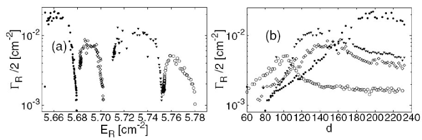
Figure 1: Resonance position for four resonances in a Sinai billiard with attached waveguide with variable opening (a) and their corresponding width $\Gamma_{R}/2$ versus the slit width $d$ (b). The different resonances are marked by different symbols (taken from reference [22]).

Different scales of lifetimes appear for the resonant states if there is sufficient overlap [70, 71, 72]. Some of the states align with the decay channels and become short lived, while the remaining ones decouple from the continuum and become long lived, a phenomenon called trapping. The doorway states in nuclear physics provide an example for the alignment of the short-lived states with the channels [73, 74]. For a clear experimental demonstration of the trapping effect, the coupling strength to the decay channels has to be tuned. This was done experimentally by Persson et al[22], a detailed theoretical discussion can be found in [69]. In the experiment the microwaves were coupled to a resonator of the shape of a Sinai billiard via an attached waveguide, and the reflection was measured. Using a slit with variable opening width $d$ the coupling from the waveguide to the billiard could be changed. The slit width was varied in steps of 0.1 mm from 60 to 240 mm. Resonance positions and widths were extracted using a centered time-delay analysis [22]. In figure 1(a) the dependence of four resonance positions on the opening $d$ of the slit is shown. In figure 1(b) the width $\Gamma$ is plotted as a function of the slit opening $d$. For small slit openings $d$ the widths of the resonances first increase with $d$ but for larger openings the width finally decrease again, thus demonstrating the effect of resonance trapping [22].

In the case of resonance trapping all resonances are treated on equal footings. If there is only an overlap of two resonances and all others resonances are far apart one can describe the occurring pattern in the transmission by Fano resonances [75, 76]. Fano resonances have been observed originally in photoabsorption in atoms [77, 78, 79] but occur in many fields in physics like electron and neutron scattering [80, 81], Raman scattering [82], photoabsorption in quantum well structures [83], scanning tunnel microscopy [84], and ballistic transport through quantum dots ( artificial atoms ) [85, 86, 87, 88]. Close to a given resonance $E_{i}^{R}$ the spectra can be approximated by the Fano form [79, 89],

$$|T(E,d)|^{2}\approx\frac{|E-E_{i}^{R}(d)+q_{i}(d)\Gamma_{i}(d)/2|^{2}}{\left[E-E_{i}^{R}(d)\right]^{2}+\left[\Gamma_{i}(d)/2\right]^{2}}$$ (37)

where $d$ describes the coupling strength, $E_{i}^{R}(d)$ is the position of the $i$th resonance, $\Gamma_{i}(d)$ its width, and $q_{i}(d)$ the complex Fano asymmetry parameter. Window resonances appear in the limit $q\rightarrow 0$ while the Breit-Wigner limit is reached for $|q|\gg 1$ (see reference [90] for details). It should be noted that, in general, $q$ cannot be simply identified with the ratio of resonant to non-resonant coupling strength [89, 91, 92]. Moreover, since Fano resonances result from the interference between resonances related to the eigenmodes in the cavity, the parameter $q$ depends very sensitively on the specific constellation of the involved resonance poles [75, 76].

In none of the previously mentioned experiments the Fano resonances could be systematically studied by varying the coupling strength. Again this has been achieved in a microwave billiard [90, 93]. The setup consisted of two commercially available waveguides which were attached centred both to the entrance and the exit side of a rectangular resonator. At the junctions to the cavity metallic apertures of different openings $d$ were inserted. In the applied frequency range only two transverse modes for the rectangular cavity could be excited. A continuous transition from a narrow Breit-Wigner ($q$ very large, $d$ small) to a window resonance ($q\to 0$, $d$ large) was found [90]. In a further investigation the effect of decoherence and dissipation on the Fano resonance lineshapes was discussed [93].

Up to now only resonances with no or weak overlap or, as in the case of the Fano resonances, with just two strongly overlapping resonances have been investigated experimentally. For a complete exploration of the features of the scattering matrix an investigation of the poles in the strong overlapping regime is needed. By means of the harmonic inversion technique [94, 95, 96, 97] this now has become possible [98].

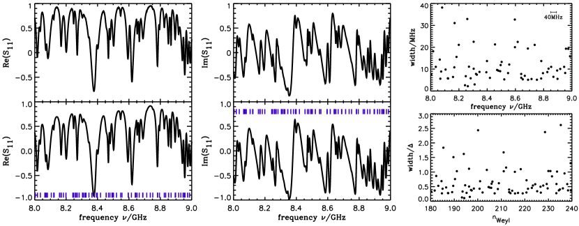
Figure 2: Left and centre: Real and imaginary part of a spectrum of a half Sinai microwave billiard with absorption. On top the measured spectrum is shown, on bottom the reconstructed spectrum as obtained from the harmonic inversion. The resonance positions are marked by short lines. Right: Resonance widths for the displayed spectra in MHz (top), and normalised to the mean level spacing (bottom) (taken from reference [98]).

In figure 2(left and centre) the complex reflection coefficient $S_{11}$ of a half Sinai billiard is shown for the frequency range from 8 to 9 GHz (for details see [98]). It is compared with a reconstructed spectrum obtained from the harmonic inversion. The resonance positions are marked by small lines. Apart from a secular overall phase shift the reconstruction is nearly perfect. Global phase shifts are not serious as long as one is only interested in resonance positions, width and absolute values of the amplitude, and their behaviour in dependence of an external parameter. On the right (top) the widths are plotted versus the frequency and (bottom) versus energy, normalised to a mean level spacings of one. In the example the resonance widths are of the order of the mean level spacing $\Delta$, but it was possible to penetrate into regimes where the resonance width amounted up to about ten times the mean level spacings. For isolated resonances one expects a Porter-Thomas distribution [99, 1], whereas for strong coupling the tails of the distribution decay according to $P_{\Gamma}(\Gamma)\propto\Gamma^{-2}$ [100, 101]. This could be verified in the experiment [98].

3.3 Distribution of reflection and transmission coefficients

The first experimental investigation of scattering theory was done by Doron et alwho studied the reflection properties of an elbow system [17]. It concentrated on the influence of the classical escape behaviour on the reflection, and will be treated in subsection 3.6 in the proper context. It took about ten more years until the influence of coupling and absorption was investigated experimentally by several groups in microwave billiards in more detail [102, 103, 24, 104, 105, 106]. Barthélemy et aldeveloped a model to describe the coupling of a microwave antenna to the system and could separate their contribution $\Gamma_{c}$ to the total resonance width $\Gamma$ from the part $\Gamma_{ohm}$ resulting from ohmic losses in the wall [24].

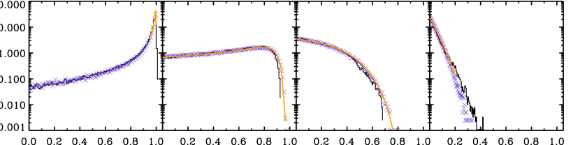
Figure 3: The distribution of the reflection $P_{R}(R)$ is shown for four different coupling strength ($T_{a}$=0.116, 0.754, 0.989, 0.998) and total absorption ($\gamma$=0.56, 2.42, 8.40, 48). Additionally the theoretical curve (yellow line) and numerical results are plotted (blue crosses) (for details see [102, 103]).

Méndez-Sánchez et alinvestigated reflection spectra in dependence of the coupling strength and the absorption [102]. The experiment was performed in a half Sinai billiard, where an additional absorbing wall could be introduced to increase the total absorption. They could verify the theoretical predictions for the limiting case of strong absorption [107]. The known result of weak absorption [108] could not be verified as it assumed perfect coupling which was not realised in the experiment. An interpolating formula for the distribution $P_{R,0}$ of reflection coefficients in the case of perfect coupling was derived [103, 109]

$$P_{R,0}(R_{0})=C_{\beta}\frac{\rme^{-{\alpha}/{(1-R)}}}{(1-R)^{2+\beta/2}}\left[A\alpha^{\beta/2-1}+B(1-R)^{\beta/2}\right],$$ (38)

with $\alpha={\gamma_{d}\beta}/{2}$, $A={\alpha}\left(\rme^{\alpha}-1\right)$, $B=(1+\alpha-\rme^{\alpha})$, $C_{\beta}=[A\Gamma(1+\beta/2,\alpha)/\alpha^{2}+B\rme^{-\alpha}/\alpha]^{-1}$ and the universality index $\beta$. $\gamma_{d}$ is a parameter describing the dissipation [103] and $\Gamma(x,\alpha)=\int_{\alpha}^{\infty}t^{x-1}\rme^{-t}dt$ is the upper incomplete Gamma function. Meanwhile there exists an exact but lengthy expression by Savin, Sommers, and Fyodorov [110]. The deviations from equation (38) are typically small. From the distribution $P_{R,0}$ the joint distribution of the reflection coefficient and the phase of the reflection coefficient ($S=\sqrt{r}\rme^{\rmi\theta}$) for incomplete coupling can be calculated via

$$P_{R,\Theta}(S)=\left(\frac{1-\langle S\rangle^{2}}{|1-S\langle S\rangle|^{2}}\right)^{2}\frac{1}{2\pi}P_{R,0}(R_{0}),$$ (39)

where $\langle S\rangle=\sqrt{1-T_{a}}$ and $R_{0}=|S_{0}|^{2}$ with $S_{0}=(S-\langle S\rangle)/(1-\langle S\rangle S)$. In figure 3 the distribution of the reflection $P(R)$ is shown for four different coupling strength $T_{a}$ and absorption $\gamma_{d}$. The theoretical curves shown in blue are obtained via a projection to the corresponding axis of $P_{R,\Theta}(S)$. A good agreement between experiment and theory is found for $P(R)$ [102, 103]. In a further work the phase distribution $P(\Theta)$, called the Poisson kernel, and the joint distribution were determined experimentally, again in perfect agreement with theory [103]. For phase distributions see section 4.6.

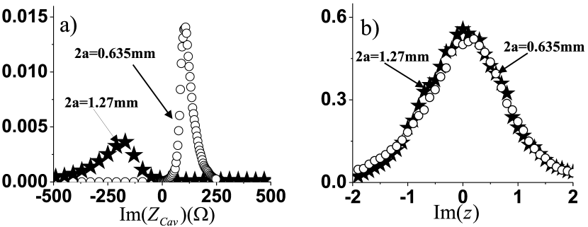
Figure 4: (a) Distribution of the imaginary part of cavity impedance for two different couplings from 9 to 9.6 GHz. (b) Rescaled plot of two curves in (a) after dividing the experimental impedances by the impedances $Z_{0}$ of the antenna (taken from reference [105]).

Hemmady et alapplied a different approach [105, 106, 111, 112]. They did not study the scattering matrix but looked for the impedance matrix $Z$ instead. These quantities are related via

$$Z=Z_{0}(1+S)/(1-S)\,.$$ (40)

$Z_{0}$ describes the coupling port and is fixed by an independent measurement. The impedance matrix relates the applied voltages $V$ to the currents at the antennas ($V=ZI$), whereas the scattering matrix relates the incoming flux with the outgoing flux. Using the impedance matrix Hemmady et alcould remove the effects of coupling thus obtaining a normalised cavity impedance, which shows a universal behaviour [105, 111]. This is demonstrated by figure 4.

Microwave graphs are another possibility to study the influence of absorption on the distribution of reflection coefficients, real and imaginary part of impedances etc. This has been done by Hul et al[113]. Again a perfect agreement with RMT predictions was found.

Though there are no analytical results available for the joint distribution of scattering matrix elements for more than one channel, apart from the distribution of the modulus of the eigenvalues [114], there are results for the distribution of the total transmission $T$. This quantity is of practical interest, since due to the Landauer formula the total transmission through an open quantum dot is, up to an universal vector, nothing but the conductance $G$,

$$G\sim T=\sum\limits_{n,m}\left|S_{nm}\right|^{2}\,,$$ (41)

where the index $n$ sums over all incoming and the index $m$ over all outgoing channels. There are a number of predictions on the distribution $p(T)$ of the transmission in dependence of the channel number for systems with and without time-reversal symmetry [115, 116]. In the calculation the matrix elements had been assumed to be Gaussian distributed, and uncorrelated, apart from the constraint of the universality of the $S$ matrix. The assumption of Gaussian distributed scattering matrix elements seems to be in contrast to expression (4) for the scattering matrix. It can be shown, however, that for chaotic cavities and perfect coupling both approaches are equivalent [117] (see section IIA.4 of reference [118] for a discussion). Experimentally obtained conductance distributions for quantum dots were in serious disagreement with the calculations, though the influence of the break of time reversal symmetry could be qualitatively reproduced [119]. A possible problem arises from the fact, that the geometry of the dots defined by the gate electrodes is ill-defined, and thus the channel number as well.

In microwave cavities this problem does not exist. Experiments have been performed in a chaotic cavity with two attached waveguides both on the entrance and the exit side. Time reversal symmetry was broken by inserting ferrite cylinders. The phase-breaking mechanism of the ferrite can be qualitatively understood as follows: Applying a magnetic field, the electronic spins in the ferrite perform a precession with the consequence that microwaves reflected from a ferrite surface experience a phase shift whose sign depends on the direction of propagation. This effect has been used previously by So et al[120] and Stoffregen et al[121] to study time-reversal symmetry breaking in closed microwave billiards. However, the ferrite introduces strong absorption, and the phase-breaking effect is present only in a narrow frequency window in the wing of the ferromagnetic resonance. Thus the calculation of the transmission distribution has to be modified by introducing additional absorbing channels. If this is done, both the break of time-reversal symmetry and the channel number dependence can be well reproduced by the calculations [122].

3.4 Correlations of $S$ matrix elements

The Fourier transform of the spectral autocorrelation function

$$C(E)=\left<\rho(\bar{E})\rho(\bar{E}+E)\right>-\left(\left<\rho(\bar{E})\right>\right)^{2}\,,$$ (42)

yields the spectral form factor

$$K(t)=\int_{-\infty}^{\infty}C(E)\exp\left(-\frac{\imath}{\hbar}Et\right)\,dE\,.$$ (43)

In chaotic systems $K(t)$ shows a hole for small values of $t$, resulting from the spectral rigidity. Extensive work on the spectral hole has been done, among others in nuclear physics [123] and in the analysis of spectra from microwave cavities [124]. The spectral hole is thus a convenient indicator to test chaotic behaviour.

In open systems the spectral autocorrelation function has to be replaced by scattering matrix correlation functions

$$C[S^{*}_{ab},S_{cd}](E)=\langle S^{*}_{ab}(\bar{E})\,S_{cd}(\bar{E}+E)\rangle-\langle S^{*}_{ab}(\bar{E})\rangle\;\langle S_{cd}(\bar{E})\rangle\,,$$ (44)

or, alternatively, by their Fourier transforms

$$\hat{C}[S^{*}_{ab},S_{cd}](t)=\langle\hat{S}^{*}_{ab}(t)\,\hat{S}_{cd}(t)\rangle-\delta(t)\langle S^{*}_{ab}(\bar{E})\rangle\;\langle S_{cd}(\bar{E})\rangle\,,$$ (45)

where

$$\hat{S}_{ab}(t)=\int_{-\infty}^{\infty}S_{ab}(E)\exp\left(-\frac{\imath}{\hbar}Et\right)\,dE$$ (46)

.

The optical theorem

$$\sigma_{\rm tot}^{(a)}=2\left(1-{\rm Re}S_{aa}\right)$$ (47)

establishes a relation between the diagonal elements of the scattering matrix and the total cross section, often used in nuclear physics. Correlation functions of the diagonal elements of the scattering matrix may thus be alternatively expressed in terms of correlation functions of the total cross section [125].

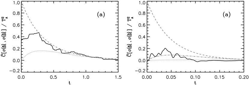
Figure 5: Normalized cross-correlation function $\hat{C}[\sigma_{\rm tot}^{(a)},\sigma_{\rm tot}^{(b)}]$ for (a) a rectangular and (b) a chaotic billiard with $C_{3}$ symmetry with the Fourier transform taken over the frequency range 13 to 14 GHz (the division by $T_{A}^{2}$ accounts for the antenna coupling, see the original paper for details). Dotted and dashed lines are theoretical results for GOE and POE, respectively, taking absorption into account. The dash-dotted line in (b) corresponds to the theoretical expectation for the $C_{3}$ billiard (for details see the original work) (taken from reference [126]).

As an example figure 5 shows the cross correlation for a rectangular and the chaotic cavity, obtained from reflection measurements at two different antennas [126]. There was a strong absorption, which had to be considered in the theory. Whereas for integrable systems an exponential decay of the correlation function is expected, caused by the absorption, for chaotic systems the correlation is always close to zero, thus exhibiting the correlation whole. In both cases the experimental results follow the predictions. Discrepancies are found only for the rectangular billiard for small times. They are caused by the presence of the antennas making the systems pseudo-integrable and producing a small correlation hole which is absent in the ideal rectangle [127].

An experimental observation of the correlation hole in the regime of visible light has been achieved by Dingjan et al[11]. The authors studied a transmission spectrum of a He-Ne laser through an open resonator made up of two end mirrors, either curved or flat and a curved folding mirror. By misaligning the latter one very large aberrations could be introduced thus making the system chaotic. Taking the Fourier transform of the spectral autocorrelation functions both for the regular and the disturbed system, curves were obtained very similar to the ones shown in figure 5 for the microwave system.

Very recently the study of scattering matrix correlation functions has been extended to the subject of fidelity. The fidelity amplitude is defined as the overlap integral of some initial state with itself after the evolution under the influence of two slightly different time evolution operators $U(t)$, $U^{\prime}(t)$,

$$f(t)=\left<\psi(0)\right|U^{\dagger}(t)\,U^{\prime}(t)\left|\psi(0)\right>$$ (48)

The modulus square of the fidelity amplitude, the fidelity $F(t)=|f(t)|^{2}$, had been proposed years ago by Peres to quantify the stability of a quantum-mechanical system against perturbations [128]. The renewed interest in the topic results from its relevance for quantum-information processing. The fidelity amplitude as defined in equation (48), is experimentally hardly accessible, as it requires the knowledge of the complete wave function. This was the motivation by Schäfer et al[129], to introduce a scattering fidelity, defined in terms of scattering matrix elements of the perturbed and unperturbed system. In the weak coupling limit the scattering fidelity approaches the ordinary fidelity (48). Perturbation theory predicts an exponential decay of the fidelity for $t<t_{H}$, and a cross-over to a Gaussian decay for $t>t_{H}$. $t_{H}=\hbar/\Delta E$ is the Heisenberg time, where $\Delta E$ is the mean level spacing [130].

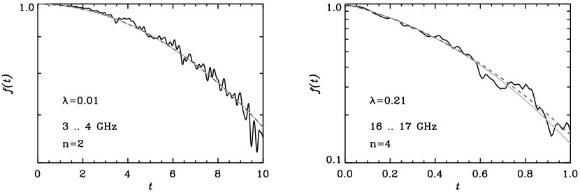
Figure 6: Fidelity amplitude for a chaotic microwave billiard. The smooth solid line shows the linear-response result, while the dashed line corresponds to the exact result. The perturbation parameter $\lambda_{\rm exp}$ has been fitted to each experimental curve (see the original work for details) (taken from reference [129]).

In a microwave experiment the perturbation was achieved by moving one wall in a chaotic microwave resonator with two attached antennas. In addition averaging was performed by superimposing the results from different energy window and geometries. Figure 6 shows the result for different perturbations. For small perturbations the Gaussian decay dominates, whereas with increasing perturbations strength a cross-over to an exponential decay is observed. In the range accessible to the experiment a good agreement was found with a linear-response prediction of random matrix theory [131]. Deviations of the linear response results from the exact results, obtained by super-symmetry techniques [132, 133] amount to at most 10 percent in the regimes shown in the figure, which could not be detected in the experiment.

Essentially the same results have been obtained in an experiment in elastodynamic billiards [134]. They will be presented in section 4.3.

3.5 Current correlations

A systems has to be opened if a measurement is to be performed. As a consequence the eigenvalues are turned into resonances and acquire widths. This has been investigated in the previous subsections. Now we want to investigate the effect of the openings on wave functions and currents. Due to the openness the wave function acquires an imaginary part, i. e.,

$$\psi=\psi_{r}+\rmi\psi_{i}.$$ (49)

A convenient parameter to characterise the openness is the phase rigidity $|\rho|^{2}$ of $\psi$ [135], where

$$\rho=\int\rmd\bi{r}\,\psi(\bi{r})^{2}=\frac{\langle\psi_{r}^{2}\rangle-\langle\psi_{i}^{2}\rangle}{\langle\psi_{r}^{2}\rangle+\langle\psi_{i}^{2}\rangle}\,.$$ (50)

$\rho$=1 corresponds to the closed and $\rho$=0 to the completely open system.

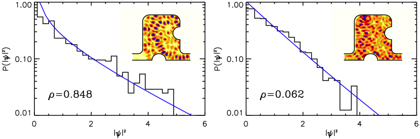
Figure 7: Intensity distribution $P_{\rho}(I)$ for two different values of rigidity $\rho$. The insets show the corresponding intensity pattern $I=|\psi|^{2}$ for a quantum dot like microwave billiard.

The random plane wave approach introduced in section 2.2 allows to calculate the intensity distribution. In open systems the amplitudes $a(\bi{k})$ (see equation (12)) obey the relation $\langle a(\bi{k})a(-\bi{k})\rangle=\rho\langle a(\bi{k})a^{*}(\bi{k})\rangle$. For a fixed value of $\rho$ this implies a generalised Porter-Thomas distribution for the intensity,

$$P_{\rho}(I)=\frac{1}{\sqrt{1-|\rho|^{2}}}\exp\left[-\frac{I}{1-|\rho|^{2}}\right]I_{0}\left[\frac{|\rho|I}{1-|\rho|^{2}}\right],$$ (51)

In figure 7 the intensity distribution for a microwave billiard with attached leads is plotted. The transitional behaviour from a closed system to an open system is clearly visible [136]. Good agreement with the theoretical prediction is found, where the only free parameter $\rho$ is taken directly from the data.

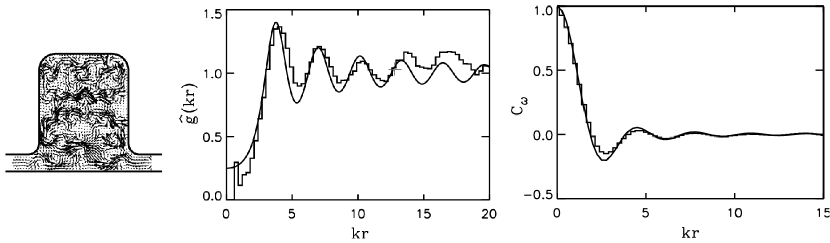
Figure 8: Left: Typical probability current pattern. Centre: Experimental vortex pair correlation function $\hat{g}$, together with the theoretical prediction. Right: vorticity spatial autocorrelation function (taken from reference [137]).

For closed systems there is a large interest in nodal lines (see e. g. [138]), whereas in open systems there exists only nodal points. The nodal points correspond to vortices of the quantum mechanical probability density

$$\bi{j}(\bi{r})=\frac{A}{k}{\rm Im}[\psi^{*}(\bi{r})\nabla\psi(\bi{r})].$$ (52)

At the same time the vortices give rise to phase singularities which have been demonstrated in a rectangular microwave billiard with an introduced absorber [139]. There are a number of theoretical results on the distribution of the modulus of the currents $j$ or its components $j_{x}$, $j_{y}$ [140], vortex spacing distributions [141, 142], various spatial autocorrelation functions etc., using the plane wave approximation. In quasi-tow-dimensional systems there is a one-to-one correspondence between the quantum probability current and the Poynting vector [139], allowing to determine the flow patterns experimentally. The left part of figure 8 shows a typical example. This has been used to verify these distributions and correlation functions by microwave experiments [143, 137]. In the central figure 8 the vortex pair correlation function is shown, together with the prediction from the random plane wave approximation [144, 141]. In the right part of the figure the spatial autocorrelation function of the vorticity $\omega=(1/2)\bi{[\nabla\times j]}$ is shown, again together with the theoretical prediction. In both examples a good agreement between theory and experiment is found.

Usually spatial correlations vanish for $kr\to\infty$. Therefore it came as a surprise when Brouwer showed that there exist a number of correlation functions with long-range correlations [145], i. e., with a surviving correlation in the limit $kr\to\infty$. This is the case, e. g. for the connected correlator of the squared intensity, $\langle I(\bi{r})^{2}I(\bi{r}^{\prime})^{2}\rangle_{c}$ showing a surviving correlation of $\mathrm{var}|\rho|^{2}$ for $kr\to\infty$ (the subscript “$c$” refers to the connected correlator, $\langle AB\rangle_{c}=\langle AB\rangle-\langle A\rangle\langle B\rangle$). The long-range correlation was experimentally verified for various correlators [136].

3.6 Classical phase space signatures of scattering

In the preceding section we discussed some universal properties of the scattering matrix. In the following a number of features shall be presented associated with individual system properties. The basis for the semi-classical treatment of scattering is an expression for the scattering matrix originally given by Miller [146],

$$S(\bi{r},\bi{r}\,^{\prime},k)=\sum\limits_{n}w_{n}e^{\frac{\imath}{\hbar}S_{n}}\,,$$ (53)

where the sum is over all classical trajectories from $\bi{r}$ to $\bi{r}\,^{\prime}$. $w_{n}$ is a stability factor, which can be calculated from the classical dynamics, and $S_{n}$ is the classical action. For billiard system $S_{n}$ is given by $S_{n}=\hbar kl_{n}$, where $l_{n}$ is the length of the trajectory. Equation (53) can be looked upon as a special result of Gutzwiller’s semi-classical quantum mechanics, expressing the Green’s function in terms of classical trajectories [147].

In billiards systems the Fourier transform of equation (53), with $k$ as the variable, gives the stability weighted length spectrum. This has be used by Kim et al[148, 137] in a number of papers to test a conjecture that the transport in quantum dots is mainly promoted via scarred wave functions. In a soft-walled microwave billiard the same authors found evidence for dynamical tunneling, i. e. quantum-mechanical cross-talking between stable islands in phase space being classically separated [149].

For a large number of open channels the scattering matrix in the time domain decays exponentially with a time constant $\tau$, resulting in a Lorentzian shape of the corresponding autocorrelation function with width $\Gamma=1/\tau$, see equation (19). Semiclassical theory identifies $\tau$ with the classical escape rate [150, 151]. This was the issue of the first microwave experiment on scattering in an elbow-shape resonator, where, however, the number of open channels was not large but just one. Lu et al[152] studied the spectral autocorrelation function in an $n$-disc scattering system with $n=1,2,3,$ and found a perfect agreement between the observed width and the values expected from the classical escape weight.

A characteristic feature of the $n$-disc system is a classical repeller associated with a bouncing ball orbit between two neighbouring discs. It follows from semiclassical theory that the decay of the scattering matrix is no longer single-exponential but given by a superposition,

$$\hat{C}_{ij}(t)=\sum\limits_{n}a_{n}\rme^{-\gamma_{n}t}\cos({\gamma_{n}}^{\prime}t)\,.$$ (54)

where ${\gamma_{n}}^{\prime}$ and $\gamma_{n}$ are real and imaginary part of the eigenvalues of the Frobenius-Perron operator describing the classical dynamics of the system. The corresponding autocorrelation function shows the so-called Ruelle-Pollicott resonances.

These resonances have been studied by Pance et al[153] for the $n$-disk system for $n=1,2,3$. In all cases the found resonances were in perfect agreement with those expected from the classical dynamics.

Another scattering experiment showing clear fingerprints of the underlying classical dynamics has been performed by Dembowski et al[154]. The authors studied the transport of microwaves through a channel confined from above by a Gaussian and from below by an inverted parabola. The dominant structure of the associated Poincarè section, taken at either boundary, is a stable island associated with the bouncing ball orbit along the symmetry line of the channel. This region is classically not accessible. The trajectories surround instead the stable island repeatedly in phase space, before they leave the channel either to the left or the right side. This revolution show up in a lighthouse-like oscillatory decay of the scattering matrix on the time domain.

3.7 Summary

Up to about 1990 the study scattering was essentially a domain of theory. Noticeable exceptions were the spectra of compound nuclei giving rise to the development of random matrix theory [1]. The situation changed completely with the emergence of different types of billiard experiments. After the first microwave study [7] there were numerous experiments with classical waves and quantum dots [16]. In microwave experiments, in contrast to quantum dots, there is a complete control over the geometric parameters. Therefore a quantitative agreement between experiment and random matrix predictions was achieved for all cases studied up to now. To this end it was necessary, however, to take absorption and imperfect coupling into account which was ignored in most previous investigations. Fortunately there has been quite a large number of theoretical studies in recent years to close this gap ([155], this volume), motivated last but not least by the possibility to test the theoretical predictions experimentally.

4 Experiments with sound waves

4.1 Measurements of eigenstatistics in acoustics

Manfred Schröder [40] appears to have been the first to note that RMT level statistics should apply to acoustic systems and could have implications for room acoustics and for structural vibration. Interestingly, in his thesis he used microwaves in order to conduct experiments that would be analogous to an acoustic system. Weaver [46, 47] was the first to measure RMT statistics in acoustics. He determined about 150 elasto-dynamic levels in each of three small aluminum blocks excited by impulsive forces and measured in the time domain with piezoelectric detectors. Acoustic systems often lend themselves naturally to time-domain measurements. Such measurement are related by Fourier transform to the frequency sweeps typically done on microwave billiards. Ellegaard and several co-workers repeated these measurements, and extended them [48, 49]. Here Ellegaard et almeasured $\sim$ 300 resonances in each of several aluminum blocks with varying spherical octants of material removed from a corner. Sub-Poissonian level statistics were observed in the less irregular samples and ascribed to mode conversions. Statistics approached the GOE as more material was removed. The work was extended to quartz blocks [50], of higher $Q$, with the identification of about 1400 levels. Again various sized octants of material were removed from the corner, thus allowing a study of the transition between a sub-Poissonian and a GOE case. Neicu and Kudrolli [156] also studied the evolution of eigenstatistics under shape deformations.

Later work from the Copenhagen group emphasized studies of 2-d plate-structures, analogous to the microwave billiard experiments conducted by many others. At sufficiently low frequency or small thickness of the plate it has only flexural and in-plane modes, which may or may not be coupled depending on the breaking of up/down symmetry. Bertelsen et al[157] studied nearly 1000 levels of a Sinai-stadium plate and found good agreement with a Weyl-like estimate of level density, and, if up/down symmetry is broken, good agreement with RMT predictions for other level statistics. Andersen et al[49] showed how variations in air-pressure on such plates allows to distinguish between flexural waves (with non-negligible losses to air) and in-plane modes (with low losses to air). Once distinguished in this manner, the level statistics of the two kinds of modes could be separately shown to be GOE.

Level dynamics, under variation of a parameter, has attracted attention also. Not only can one study the evolution of statistics as a system changes its symmetry or integrability, RMT also makes predictions for the (scaled) distribution of level curvatures as a parameter is varied. Bertelsen et al[51] studied the ’Devil’s spaghetti’ formed by the level dynamics under variations in temperature.

At a lower confidence level, due to lower $Q$ systems and few modes identified, others also have confirmed GOE level statistics in vibrations and acoustics, [35, 45]

The spatial statistics of diffuse fields in general and modes in particular, have also attracted attention. There are a few measurements directly imaging mode shapes, and a few of more generic diffuse fields. More commonly such statistics are investigated implicitly by means of field correlations amongst a discrete set of points.

4.2 Spatial correlations

Ebeling and Rollwage et al[34, 27] discussed measurements of diffuse waves in reverberation rooms and in 2-d ripple tanks and showed agreement with predictions based on the random plane-wave superposition argument. In particular they showed that field-field correlations $\langle\psi(\bi{x})\psi(\bi{x}+\bi{r})\rangle=J_{0}(k|r|)$, and that intensity-intensity correlations were the expected $\langle I(\bi{x})I(\bi{x}+\bi{r})\rangle=2J_{0}^{2}(k|r|)+1$. The particular virtue of ripple tanks is ready imaging of wavefields. Chinnery [9] has also presented pictures of (2-d) acoustic modes in water. Similar studies have been made on drum heads [35], and capillary waves [8].

Schaadt et al[57] studied mode shapes and their statistics in a plate with flexural and in-plane modes. By scanning their needle-like piezoelectric sensor, they could map a component of the surface displacement field of any mode of their choice. By means of pressure variations, they could determine if the mode in question was flexural or in-plane (or a mixture if the plate lacked up-down symmetry.) They showed the expected $1+2J_{0}^{2}$ intensity-intensity ($I$-$I$) statistics amongst the flexural waves, and an expected more complex relation for the $I$-$I$ statistics of the in-plane modes. The complexity is due to the mixture of wave speeds associated with such modes [58].

Several works of late have reported theory and measurements of diffuse-field-diffuse field correlations with features beyond the well-known $J_{o}$ behaviour. These features are somewhat weaker and more difficult to discern than the short-distance $J_{o}$, but they are non-universal and of some practical importance. While this work has generally been confined to correlations amongst generic fields, one imagines that they apply also to modes.

Weaver [158, 159] showed that the field-field correlation function in a reverberant body was the (imaginary part of the) Green’s function. This is essentially equivalent to a correlation between S matrix elements $\langle S_{ij}(\omega)S_{kj}^{\ast}(\omega)\rangle$. The correlation reduces to $J_{0}$ in the interior of a large 2-d single wave speed isotropic billiard, but has other features in more complex bodies, or near boundaries or scatterers. In particular it retains signatures associated with reflections from nearby heterogeneities. Weaver derived this from a modal perspective [158, 159] using assumptions on modal statistics, but it has also been derived in other ways. Derode [160] showed that this relation is closely related to time-reversed acoustics. An example, taken from [161] and plotted in figure 9, shows how a conventional waveform, with sharp arrivals in the time domain related to strong reflections, emerges from correlations of a diffuse field. Campillo et al[162, 163, 164] have used such correlations to map the earth’s surface structure using seismic waves. The ability to retrieve the Green’s function by passive measurements is gathering attention in ocean acoustics and seismology [162, 163, 164, 165, 166].

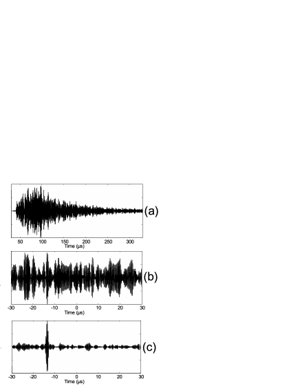
Figure 9: A transient diffuse field in a multiply scattering water tank (a) is autocorrelated (b). On averaging (b) over 118 distinct distant sources, a sharp arrival appears. The sharp feature appears at a time corresponding to a retroreflection from a nearby heterogeneity, as would be seen if the receiver were used in pulse-echo mode (taken from reference [161]).

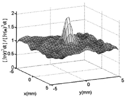
Figure 10: The enhanced backscatter peak near the position of the source in a 2-d chaotic elastic wave billiard was imaged by de Rosny et al(taken from reference [55]).

4.3 Fidelity

In section 3.4 the concept of scattering fidelity was introduced to account for the fact that fidelity as originally defined is not accessible to the experiment. It was shown that under the assumptions of ergodicity the two definitions of fidelity are the same [167, 132]. Snieder introduced the notion of ‘coda-wave interferometry’ in seismology [168] equivalent to scattering fidelity. Weaver and Lobkis independently studied the same idea in ultrasonics [134] where temperature changes were responsible for the changed Hamiltonian. De Rosny et al[169] looked at a similar effect with acoustic waves in a tank with moving scatterers. Snieder applied it to ultrasonics in rock [168] and showed an effect from temperature variations and from the opening of a crack. Weaver and Lobkis [134] showed that the measurement could be used to evaluate the mixing rates of different waves. In particular they showed that a regular body had much lower fidelity than did a ray-chaotic body. They confined their quantitative evaluations to times short compared to the Heisenberg time. Later Gorin et al[170] showed that RMT theory for the time dependence on the scale of the Heisenberg time was consistent with Weaver and Lobkis’s measurements over such times.

Ribay et alhave considered the effect of temperature variations on reverberant acoustic signals in water and in air and on flexural waves in plates [171]. To the extent that temperature changes in these systems merely change wave speed and volume, and do so homogeneously, the only effect of such changes is to dilate the waveforms. This trivial effect is not difficult to account for. Because longitudinal and shear wave speeds have different dependencies on temperature, in elastic bodies there is also a nontrivial change of waveform [134].

Lu and Michaels [172] have suggested that ultrasonic fidelity, after correction for temperature variations, may be useful as a nondestructive means for monitoring the condition of materials and built structures. Growth of a crack for example will degrade fidelity [168], and do so in a manner depending on the size and position of the crack.

Lobkis (unpublished) has measured the almost perfect fidelity of ultrasonic waveforms under the addition of a very weakly coupled loss channel, and shown extraordinary sensitivity to that addition, far greater than that exhibited by the energy dynamics (see below)

Figure 11: Measurements of the free decay of intensity $|S(t)|^{2}$. It is found that the Breit-Wigner formula (36) and its generalizations (dashed lines), often do not match measurements. A full RMT calculation (solid lines) does match. Differences are most pronounced when channels are well coupled (taken from reference [21]).

4.4 Reflection and Transmission Distributions

Coherent backscattering, i. e., enhancements of the diagonal elements of $G$ or $S$, are most profitably studied in the time domain. Acoustics is thus a natural way to examine it. Coherent backscatter enhancements by factors varying in time from two and three are readily observed: $|S_{ii}|^{2}\sim(2$ to $3)\times|S_{ij}|^{2}$ $(i\neq j)$. Lyon [44] was the first to predict enhanced backscatter in acoustics, followed much later by a prediction of its dynamics by Weaver and Burkhardt [173] using a modal perspective and assumed GOE modal statistics. It was first observed in acoustics by de Rosny et alin a 2-d billiard [55] (See fig. 10) and by Lobkis and Weaver in a 3-d billiard [174]. Larose et al[175] observed enhanced backscatter with seismic waves in an open multiply scattering system, with potential for application to characterizing the earth.

A system consisting of two or more weakly coupled cavities can exhibit an enhanced backscatter that is a form of Anderson localization; all elements $S_{ij}$ or $G_{ij}$ with $i$ and $j$ within the same substructure are enhanced, by arbitrarily large factors, relative to others. This was observed by Lobkis and Weaver [176] in a system consisting of two coupled reverberant elastic bodies. It has been analyzed theoretically by Weaver and Lobkis [176] and by Gronqvist and Guhr [177]

In a non-lossy system, responses are given simply in terms of real modes and real natural frequencies. Spectra $|S_{ij}(\omega)|^{2}$ consist of distinct resonances; interpretation of spectra is straightforward. In the presence of loss these resonances spread and at high enough loss, they overlap, thus complicating interpretation of power spectra. At very high loss where the modes are well overlapped, the statistics simplify; they become equivalent to Ericson fluctuations [31]; responses in the time domain can be understood as simply decaying coloured Gaussian random processes. Frequency domain response statistics are derived from that picture by Fourier transform.

Statistics at intermediate overlap are not as well understood. Most acoustics has concentrated on the question of the variance of power transmission $|S_{ij}(\omega)|^{2}$ for $i\neq j$, (as opposed to its distribution as in section 3.3) These may be considered intensity-intensity statistics, and thus an extension of the field-field statistics of the previous section. Lyon [44] early appreciated that these random spectra were relevant to reverberation rooms and structural vibrations. He made theoretical estimates for the intensity variance by expressing responses in the modal form (28), and taking expectations of $|G|^{2}$ written in terms of sums of various products of four modal factors. The square of the intensity $T=|G|^{2}$ transmitted from a source at $y$ with polarization $j$ to a receiver at $x$ with polarization $i$ is given, after a few minor approximations and simplifications, by the modal expansion [178]:

$$T^{2}=\sum_{rmlk}\frac{u_{i}^{r}(\bi{x})u_{j}^{r}(\bi{y})}{\omega-\omega_{r}+\rmi\Gamma_{r}}\frac{\{u_{i}^{m}(\bi{x})u_{j}^{m}(\bi{y})\}^{*}}{\omega-\omega_{m}+\rmi\Gamma_{m}}\frac{u_{i}^{l}(\bi{x})u_{j}^{l}(\bi{y})}{\omega-\omega_{l}+\rmi\Gamma_{l}}\frac{\{u_{i}^{k}(\bi{x})u_{j}^{k}(\bi{y})\}^{*}}{\omega-\omega_{k}+\rmi\Gamma_{k}}$$ (55)

Under a naive assumption of simple eigenstatistics and homogeneous damping, (real modes, fixed level width) and using expressions like (55), Lyon evaluated expectations of $T$ and $T^{2}$. Waterhouse [179] and Davy [180, 181, 182] discussed and extended the analysis of Lyon. Davy carried out extensive measurements in reverberation rooms in order to corroborate such predictions, and found some limited success. Weaver [183] pointed out that consideration of spectral rigidity neglected by Lyon and Davy would improve agreement, but that discrepancies would remain. Lobkis et al[178] re-developed the modal-expansion theory for variance of $T$ using exact GOE level and mode statistics. They also incorporated the effect of a level width distribution and consequent decay curvature. For lack of any other model, they retained the assumption of real eigenmodes, with modal statistics identical to those of the GOE.

Like that of Davy, their theory consistently overestimated variance relative to measurements on ultrasound in reverberant elastic bodies, see figure 12. They ascribed the discrepancies to their neglect of the complexness of the eigenmodes. A detailed comparison with a direct supersymmetric RMT calculation for variance (e. g. [184]) has not yet been made.

Langley et al[185, 186] have continued to study the problem of variance in statistical structural vibration, and have presented evidence for a consistent difference between the RMT value for inverse participation ratio (three) and that observed in their structures. They furthermore conjecture that this difference may explain the differences between measured and predicted power variances.

Figure 12: The normalized variance of power transmission $|G_{ij}|^{2}$ for $i\neq j$, as measured (jagged line) in a reverberant aluminum block, and as predicted (dashed line) using a ‘naive’ theory like that of Lyon [44] or Davy [180, 181, 182] but incorporating GOE statistics on eigenvalues and real eigenfunctions, and a distribution of level widths. It is found that the naive theory consistently overestimates the variance (taken from reference [178]).

4.5 Dissipation

In dissipative systems, losses can be intrinsic to the material or the structure, or be due to explicit open channels. The first order effect of losses is to introduce a uniform exponential decay in the time domain, equivalently to add an imaginary constant to the frequency. It may be a nuisance in experiments, but the effects are trivial when viewed that way, and the theoretical questions it engenders are simple. All eigen-statistics are preserved.

In practice losses are not perfectly diagonal and there is some interesting mesoscopic physics. Dissipation is often distributed nearly homogeneously, so deviations from the predictions of simple theory are small; they are nevertheless observable. Three major non-trivial topics have been addressed. The simplest is perhaps that of ‘decay curvature’ [187, 188, 61, 62, 63] (discussed below) in which a variance of level widths manifests as a non-exponential decay of intensity in the time domain as in equation 18 and 36. In the frequency domain this manifests in field-field correlations $\langle S_{ij}(\omega)S_{ij}^{*}(\omega+\Omega)\rangle$ (see section 4.2). There are also studies of transmission power variances $\langle|S|^{4}\rangle-\langle|S|^{2}\rangle^{2}$ (see section 4.4) and of complex modes (see section 4.6).

Decay curvature (36) was derived in acoustics by Schröder [60] and later by Burkhardt [61, 62, 63]; it is based on a Breit-Wigner expression for level widths (15), (25) (It was discussed for microwaves in eqn. 8). Burkhardt [61, 62, 63] found good agreement between observed decay curvatures and the formula (36) and furthermore found that $\nu$ correlated with the number of sites of material damage in a reverberant body. Weaver and Lobkis [21] and Lobkis Weaver and Rozhkov [178] also found that the formula (36) does a good phenomenological job of fitting observed decay curvatures over accessible dynamic ranges. This is may be surprising, as the assumption of equally strong loss channels is surely incorrect. It is furthermore unreasonable to suppose that real modal statistics assumed in the derivation of (18) and (36) are correct. Thus Weaver and Lobkis [21] went on to show that, carefully scrutinized, decay curvature does not fit to the formula (36). They did find that a full supersymmetric RMT calculation [134] does fit the observations (see figure 11).

It is possible to understand the difference between the Breit-Wigner picture of decay curvature, equation (36) and (18), and the exact RMT result by noting that the actual modes of a lossy system are complex. Thus the conclusion that level widths are chi-square random numbers given by a sum of squares of $\nu$ equal-variance Gaussian numbers is incorrect. That sum must be replaced by a sum of $\nu$ squares of the real parts of the modes and $\nu$ squares of their imaginary parts, cf equation (25). Thus the level width distribution ought be more narrow in the presence of complex modes, and the decay curvature ought be less pronounced. RMT indeed predicts less decay curvature than does Breit-Wigner, especially for very open channels; see for example figure 11. Microwave results on non-algebraic decay have already been presented in section 3.1.

4.6 Complex eigenmodes

Non-real modes, and in particular their statistics, which have been discussed for microwaves in terms of rigidity (see section 3.4) are at present under-studied in acoustics as well. Lobkis and Weaver [59] showed that modes in moderately damped structures (where they remain discernable as they are only moderately overlapped) can have significant complexity, and that their phases have a distribution in good accordance with theoretical guesses (see figure 13). They found that observed complexities were sufficient to account for differences like those of figure 12 between naive theory and measurements. If theoretical estimates may be obtained for complex modal statistics, perhaps in terms of level width variances [104], it may be that the modal-based estimates for power variances [44, 180, 181, 182, 183, 59, 185, 186] could be brought into agreement with measurements. The distribution of resonance phases shown in figure 13b is presumably related to that of the Poisson kernel introduced for microwave systems in section 3.4, but the exact correspondence is not yet clear.

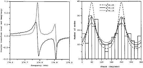
Figure 13: A short section of the real and imaginary parts of a transmission through a reverberant lossy elastodynamic body (left). It is clear that these two modes differ by a substantial phase. A histogram of the phase of resonances in this body fits well to a model of complex Gaussian modes (right) (taken from reference [59]).

4.7 Summary

In acoustics the study of response statistics has developed, over decades, mostly within the context of eigenstatistics. Theoretical predictions for field-field correlations and for intensity correlations have been formulated in terms of assumptions about the modes, with some success. It is only very recently that RMT theory and better informed measurements have been applied and the various assumptions questioned. For response statistics, as for decay curvature, a direct RMT calculation, e. g., by supersymmetry can be expected to match experimental measurements more perfectly than will an eigenmode perspective. Nevertheless eigenmode perspectives [44, 180, 181, 182, 59] that make convenient albeit incorrect assumptions about eigenstatistics have had a good deal of success. That approach to decay curvature is in most cases sufficiently accurate, and is also adequate for field-field correlations.

The eigenmode perspective for intensity variances has so far failed to accurately match measurements. If, however, such perspectives were to be extended beyond that of the most recent [178], one imagines that they might achieve an accuracy approaching that of RMT. While a full RMT treatments of systems with loss, using for example supersymmetric [184] or Monte-Carlo methods, are in principle possible, it remains desirable also to have an approach in terms of the familiar and useful and simpler concepts of eigenmodes. The estimates of Lyon, Davy, Weaver, and Langley are close enough to success to encourage the hope that such an approach may become feasible, and that a modal picture can be developed to comprehend all aspects of response statistics.

5 Summary

It is not unusual in science that related concepts are developed independently in different fields without mutual knowledge of each other. This is particularly true for scattering theory. The example of Ericson fluctuations in nuclear physics on the one hand, and universal conductance fluctuations in mesoscopic physics on the other hand, and universal power transmission coefficient fluctuations in acoustics, have already been mentioned. Another example is the random plane wave approximation which was proposed independently in the quantum mechanics of chaotic systems [28] and in acoustics [27]. Also the concept of fidelity has been independently developed in both fields, though using different notions. It has been the motivation for this review to illustrate the underlying concepts common to all types of classical waves, with special emphasis on microwaves and sound waves.

R. W. was supported by the NFS and H.-J. St. and U. K. by the DFG.

References

References

- [1] Porter C E 1965 Statistical Theory of Spectra: Fluctuations (New York: Academic Press)
- [2] Mahaux C and Weidenmüller H A 1969 Shell-Model Approach to Nuclear Reactions (Amsterdam: North-Holland)
- [3] Casati G, Valz-Gris F and Guarneri I 1980 Lett. Nuov. Cim. 28 279
- [4] Bohigas O, Giannoni M J and Schmit C 1984 Phys. Rev. Lett. 52 1
- [5] Blümel R and Smilansky U 1990 Phys. Rev. Lett. 64 241
- [6] Weaver R L 1989 J. Acoust. Soc. Am. 85 1005
- [7] Stöckmann H J and Stein J 1990 Phys. Rev. Lett. 64 2215
- [8] Blümel R, Davidson I H, Reinhardt W P, Lin H and Sharnoff M 1992 Phys. Rev. A 45 2641
- [9] Chinnery P A and Humphrey V F 1996 Phys. Rev. E 53 272
- [10] Doya V, Legrand O, Mortessagne F and Miniatura C 2002 Phys. Rev. Lett. 88 014102
- [11] Dingjan J, Altewischer E, Exter M and Woerdman J P 2002 Phys. Rev. Lett. 88 064101
- [12] Gensty T, Becker K, Fischer I, Elsäßer W, Degen C, Debernardi P and Bava G P 2005 Phys. Rev. Lett. 94 233901
- [13] Marcus C M, Rimberg A J, Westervelt R M, Hopkins P F and Gossard A C 1992 Phys. Rev. Lett. 69 506
- [14] Fromhold T M, Eaves L, Sheard F W, Leadbeater M L, Foster T J and Main P C 1994 Phys. Rev. Lett. 72 2608
- [15] Crommie M F, Lutz C P, Eigler D M and Heller E J 1995 Physica D 83 98
- [16] Stöckmann H J 1999 Quantum Chaos - An Introduction (Cambridge: University Press)
- [17] Doron E, Smilansky U and Frenkel A 1990 Phys. Rev. Lett. 65 3072
- [18] Stein J, Stöckmann H J and Stoffregen U 1995 Phys. Rev. Lett. 75 53
- [19] Alt H, Brentano P, Gräf H D, Herzberg R D, Philipp M, Richter A and Schardt P 1993 Nucl. Phys. A 560 293
- [20] Alt H, Gräf H D, Harney H L, Hofferbert R, Lengeler H, Richter A, Schardt P and Weidenmüller H A 1995 Phys. Rev. Lett. 74 62
- [21] Lobkis O I, Rozhkov I S and Weaver R L 2003 Phys. Rev. Lett. 91 194101
- [22] Persson E, Rotter I, Stöckmann H J and Barth M 2000 Phys. Rev. Lett. 85 2478
- [23] Genack A Z 2005 J. Phys. A this volume ???
- [24] Barthélemy J, Legrand O and Mortessagne F 2005 Phys. Rev. E 71 016205
- [25] Blatt J M and Weisskopf V F 1952 Theoretical Nuclear Physics (New York: Wiley)
- [26] Stein J and Stöckmann H J 1992 Phys. Rev. Lett. 68 2867
- [27] Ebeling K J Statistical properties of random wave fields volume 17 of Physical Acoustics: Principles and Methods p 233. Academic Press New York 1984
- [28] Berry M V 1977 J. Phys. A 10 2083
- [29] Hortikar S and Srednicki M 1998 Phys. Rev. Lett. 80 1646
- [30] Urbina J D and Richter K 2003 J. Phys. A 36 L495
- [31] Ericson T 1963 Ann. Phys. (N.Y.) 23 390
- [32] Schroeder M R and Kuttruff K H 1962 J. Acoust. Soc. Am. 34 76
- [33] Schroeder M R 1962 J. Acoust. Soc. Am. 34 1819
- [34] Rollwage M, Ebeling K and Guicking D 1985 Acustica 58 149
- [35] Teitsworth S W 2000 Quantum chaos effects in mechanical wave systems Proceedings of the XVI Sitges Conference on Statistical Mechanics Held at Sitges, Barcelona, Spain, 7-11 June 1999 () ed Reguera D, Platero G, Bonilla L L and Rubi J M (Berlin: Springer) p 62
- [36] Arcos E, Báez G, Cuatláyol P A, Prian M L H, Méndez-Sánchez R A and Hernández-Saldaña H 1998 Am. J. Phys. 66 601
- [37] Kutruff H 1991 Room Acoustics (London: Elsevier Science) 3rd edition
- [38] Beranek L L 1992 J. Acoust. Soc. Am. 92 1–39
- [39] Ebeling K J, Freudenstein K and Alrutz H 1982 Acustica 51 145
- [40] Schroeder M R 1954 Acustica 4 456
- [41] Schroeder M R 1959 J. Acoust. Soc. Am. 31 1407
- [42] Schroeder M R 1969 J. Acoust. Soc. Am. 46 277
- [43] Schroeder M R 1969 J. Acoust. Soc. Am. 46 534
- [44] Lyon R H 1969 J. Acoust. Soc. Am. 45 545
- [45] Davy J 1990 Internoise 1990 International Conference on Noise Control Engineering. Inter-noise: proceedings. Poughkeepsie, NY.: Noise Control Foundation. 1 159
- [46] Weaver R 1989 J. Acoust. Soc. Am. 85 1005
- [47] Delande D, Sornette D and Weaver R 1994 J. Acoust. Soc. Am. 96 1873
- [48] Ellegaard C, Guhr T, Lindemann K, Lorensen H Q, Nygård J and Oxborrow M 1995 Phys. Rev. Lett. 75 1546
- [49] Anderson A, Ellegaard C, Jackson A D and Schaadt K 2001 Phys. Rev. E 63 066204
- [50] Ellegaard C, Guhr T, Lindemann K, Nygård J and Oxborrow M 1996 Phys. Rev. Lett. 77 4918
- [51] Bertelsen P, Ellegaard C, Guhr T, Oxborrow M and Schaadt K 1999 Phys. Rev. Lett. 83 2171
- [52] Graff K F 1975 Wave Motion in Elastic Solids (Oxford: Dover)
- [53] Bogomolny E B and Hugues E 1998 Phys. Rev. E 57 5404
- [54] Kino G S 1987 Acoustic Waves: Devices, Imaging, and Analog Signal Processing (Englewood Cliffs, N. J.: Prentice-Hall)
- [55] de Rosny J, Tourin A and Fink M 2000 Phys. Rev. Lett. 84 1693
- [56] Draeger C and Fink M 1997 Phys. Rev. Lett. 79 407
- [57] Schaadt K, Guhr T, Ellegaard C and Oxborrow M 2003 Phys. Rev. E 68 036205
- [58] Akolzin A and Weaver R L 2004 Phys. Rev. E 70 046212
- [59] Lobkis O I and Weaver R L 2000 J. Acoust. Soc. Am. 108 1480
- [60] Schroeder M R Some new results in reverberation theory and measurement methods 5e Congres International D’Acoustique LIÉGE 7-14 Sept. p G31. 1965
- [61] Burkhardt J and Weaver R L 1996 J. Acoust. Soc. Am. 100 320
- [62] Burkhardt J 1997 J. Acoust. Soc. Am. 102 2113
- [63] Burkhardt J 1998 Ultrasonics 36 471
- [64] Alt H, Brentano P, Gräf H D, Hofferbert R, Philipp M, Rehfeld H, Richter A and Schardt P 1996 Phys. Lett. B 366 7
- [65] Schardt P Mikrowellenexperimente zum chaotischen Verhalten eines supraleitenden Stadion-Billards und Entwicklung einer Einfangsektion am S-DALINAC PhD thesis Technische Hochschule Darmstadt 1995
- [66] Richter A Playing billiards with microwaves - quantum manifestations of classical chaos Emerging Applications of Number Theory (The IMA Volumes in Mathematics and its Applications, Vol. 109) ed Hejhal D A, Friedman J, Gutzwiller M C and Odlyzko A M The IMA Volumes in Mathematics and its Applications, Vol. 109 pp 479–523. Springer New York 1999
- [67] Jalabert R A, Baranger H U and Stone A D 1990 Phys. Rev. Lett. 65 2442
- [68] Schäfer R, Kuhl U, Barth M and Stöckmann H J 2001 Foundations of Physics 31 475
- [69] Stöckmann H J, Persson E, Kim Y H, Barth M, Kuhl U and Rotter I 2002 Phys. Rev. E 65 066211
- [70] Moldauer P A 1967 Phys. Rev. Lett. 18 249
- [71] Desouter-Lecomte M and Chapuisat X 1999 Physical Chemistry Chemical Physics 1 2635
- [72] Jung C, Müller M and Rotter I 1999 Phys. Rev. E 60 114
- [73] Sokolov V V and Zelevinsky V G 1997 Phys. Rev. C 56 311
- [74] Persson E and Rotter I 1999 Phys. Rev. C 59 164
- [75] Lee H W 1999 Phys. Rev. Lett. 82 2358
- [76] Magunov A I, Rotter I and Strakhova S I 2003 Phys. Rev. B 68 245305
- [77] Beutler H 1935 Z. Phys. 93 177
- [78] Fano U 1935 Nuov. Cim. 12 156
- [79] Fano U 1961 Phys. Rev. 124 1866
- [80] Adair R K, Bockelman C K and Peterson R E 1949 Phys. Rev. 76 308
- [81] Simpson J A and Fano U 1963 Phys. Rev. Lett. 11 158
- [82] Cerdeira F, Fjeldly T A and Cardona M 1973 Phys. Rev. B 8 4734
- [83] Faist J, Capasso F, Sirtori C, West K W and Pfeiffer L N 1997 Nature 390 589
- [84] Madhavan V, Chen W, Jamneala T, Crommie M F and Wingreen N S 1998 Science 280 567
- [85] Göres J, Goldhaber-Gordon D, Heemeyer S, Kastner M A, Shtrikman H, Mahalu D and Meirav U 2000 Phys. Rev. B 62 2188
- [86] Nöckel J U and Stone A D 1994 Phys. Rev. B 50 17415
- [87] Rotter S, Weingartner B, Rohringer N and Burgdörfer J 2003 Phys. Rev. B 68 165302
- [88] Kobayashi K, Aikawa H, Katsumoto S and Iye Y 2002 Phys. Rev. Lett. 88 256806
- [89] Kim D H, Sim H S and Chang K 2001 Phys. Rev. B 64 115409
- [90] Rotter S, Libisch F, Burgdörfer J, Kuhl U and Stöckmann H J 2004 Phys. Rev. E 69 046208
- [91] Kim D H, Sim H S and Chang K J 2003 Phys. Rev. B 67 129903
- [92] Eichmann U, Gallagher T F and Konik R M 2003 Phys. Rev. Lett. 90 233004
- [93] Rotter S, Kuhl U, Libisch F, Burgdoerfer J and Stöckmann H J cond-mat/0412544
- [94] Wall M R and Neuhauser D 1995 J. Chem. Phys. 102 8011
- [95] Mandelshtam V A and Taylor H S 1997 J. Chem. Phys. 107 6756
- [96] Mandelshtam V A and Taylor H S 1997 Phys. Rev. Lett. 78 3274
- [97] Main J 1999 Phys. Rep. 316 233
- [98] Kuhl U, Höhmann R, Main J and Stöckmann H J 2005 Preprint private communication
- [99] Porter C E and Thomas R G 1956 Phys. Rev. 104 483
- [100] Fyodorov Y V and Sommers H J 1997 J. Math. Phys. 38 1918
- [101] Sommers H J, Fyodorov Y V and Titov M 1999 J. Phys. A 32 L77
- [102] Méndez-Sánchez R A, Kuhl U, Lewenkopf M B C H and Stöckmann H J 2003 Phys. Rev. Lett. 91 174102
- [103] Kuhl U, Martínez-Mares M, Méndez-Sánchez R A and Stöckmann H J 2005 Phys. Rev. Lett. 94 144101
- [104] Barthélemy J, Legrand O and Mortessagne F 2005 Europhys. Lett. 70 162
- [105] Hemmady S, Zheng X, Ott E, Antonsen T M and Anlage S M 2005 Phys. Rev. Lett. 94 014102
- [106] Hemmady S, Zheng X, Antonsen Jr. T M, Ott E and Anlage S M 2005 Phys. Rev. E 71 056215
- [107] Kogan E, Mello P A and Liqun H 2000 Phys. Rev. E 61 R17
- [108] Beenakker C W J and Brouwer P W 2001 Physica E 9 463
- [109] Fyodorov Y V and Savin D V 2004 JETP Lett. 80 725
- [110] Savin D V, Sommers H J and Fyodorov Y V 2005 JETP Lett. 82 603
- [111] Hemmady S, Zheng X, Antonsen Jr. T M, Ott E and Anlage S M 2005 Preprint nlin.CD/0506025
- [112] Zheng X, Hemmady S, Jr. T M A, Anlage S M and Ott E 2005 Preprint cond-mat/0504196
- [113] Hul O, Tymoshchuk O, Bauch S, Koch P and Sirko L 2005 J. Phys. A this volume ???
- [114] Brouwer P W and Beenakker C W J 1997 Phys. Rev. B 55 4695
- [115] Baranger H U and Mello P A 1994 Phys. Rev. Lett. 73 142
- [116] Jalabert R A, Pichard J L and Beenakker C W J 1994 Europhys. Lett. 27 255
- [117] Brouwer P W 1995 Phys. Rev. B 51 16878
- [118] Beenakker C W J 1997 Rev. Mod. Phys. 69 731
- [119] Huibers A G, Patel S R, Marcus C M, Brouwer P W, Duruöz C I and Harris, Jr. J S 1998 Phys. Rev. Lett. 81 1917
- [120] So P, Anlage S M, Ott E and Oerter R N 1995 Phys. Rev. Lett. 74 2662
- [121] Stoffregen U, Stein J, Stöckmann H J, Kuś M and Haake F 1995 Phys. Rev. Lett. 74 2666
- [122] Schanze H, Stöckmann H J, Martínez-Mares M and Lewenkopf C H 2005 Phys. Rev. E 71 016223
- [123] Lombardi M, Bohigas O and Seligman T H 1994 Phys. Lett. B 324 263
- [124] Alt H, Gräf H D, Guhr T, Harney H L, Hofferbert R, Rehfeld H, Richter A and Schardt P 1997 Phys. Rev. E 55 6674
- [125] Gorin T and Seligman T H 2002 Phys. Rev. E 65 026214
- [126] Schäfer R, Gorin T, Seligman T H and Stöckmann H J 2003 J. Phys. A 36 3289
- [127] Haake F, Lenz G, Šeba P, Stein J, Stöckmann H J and Życzkowski K 1991 Phys. Rev. A 44 R6161
- [128] Peres A 1984 Phys. Rev. A 30 1610
- [129] Schäfer R, Gorin T, Seligman T H and Stöckmann H J 2005 New J. of Physics 7 152
- [130] Cerruti N R and Tomsovic S 2002 Phys. Rev. Lett. 88 054103
- [131] Gorin T, Prosen T and Seligman T H 2004 New J. of Physics 6 20
- [132] Stöckmann H J and Schäfer R 2004 New J. of Physics 6 199
- [133] Stöckmann H J and Schäfer R 2005 Phys. Rev. Lett. 94 244101
- [134] Lobkis O I and Weaver R L 2003 Phys. Rev. Lett. 90 254302
- [135] Langen S, Brouwer P W and Beenakker C W J 1997 Phys. Rev. E 55 R1
- [136] Kim Y H, Kuhl U, Stöckmann H J and Brouwer P W 2005 Phys. Rev. Lett. 94 036804
- [137] Kim Y H, Barth M, Kuhl U, Stöckmann H J and Bird J P 2003 Phys. Rev. B 68 045315
- [138] Berry M V 2002 J. Phys. A 35 3025
- [139] eba P, Kuhl U, Barth M and Stöckmann H J 1999 J. Phys. A 32 8225
- [140] Saichev A I, Ishio H, Sadreev A F and Berggren K F 2002 J. Phys. A 35 L87
- [141] Saichev A I, Berggren K F and Sadreev A F 2001 Phys. Rev. E 64 036222
- [142] Berggren K F, Sadreev A F and Starikov A A 2002 Phys. Rev. E 66 016218
- [143] Barth M and Stöckmann H J 2002 Phys. Rev. E 65 066208
- [144] Berry M V and Dennis M R 2000 Proc. R. Soc. Lond. A 456 2059
- [145] Brouwer P W 2003 Phys. Rev. E 68 046205
- [146] Miller W H 1975 Adv. Chem. Phys. 30 77
- [147] Gutzwiller M C 1990 Chaos in Classical and Quantum Mechanics Interdisciplinary Applied Mathematics, Vol. 1. (New York: Springer)
- [148] Kim Y H, Barth M, Stöckmann H J and Bird J P 2002 Phys. Rev. B 65 165317
- [149] Kim Y H, Kuhl U, Stöckmann H J and Bird J P 2005 J. Phys.: Condens. Matter 17 L191
- [150] Lewenkopf C H and Weidenmüller H A 1991 Ann. Phys. (N.Y.) 212 53
- [151] Doron E, Smilansky U and Frenkel A 1991 Physica D 50 367
- [152] Lu W, Rose M, Pance K and Sridhar S 1999 Phys. Rev. Lett. 82 5233
- [153] Pance K, Lu W and Sridhar S 2000 Phys. Rev. Lett. 85 2737
- [154] Dembowski C, Dietz B, Friedrich T, Gräf H D, Heine A, Mejía-Monasterio C, Miski-Oglu M, Richter A and Seligman T H 2004 Phys. Rev. Lett. 93 134102
- [155] Fyodorov Y V, Savin D V and Sommers H J 2005 Special Issue of J. Phys. A: Math. Gen. on ’Trends in Quantum Chaotic Scattering’ cond-mat/0507016
- [156] Neicu T and Kudrolli A 2002 Europhys. Lett. 57 341
- [157] Bertelsen P, Ellegaard C and Hugues E 2000 Eur. Phys. J. B 15 87
- [158] Weaver R L and Lobkis O I 2001 Phys. Rev. Lett. 87 134301
- [159] Weaver R L and Lobkis O I 2001 J. Acoust. Soc. Am. 110 3011
- [160] Derode A, Larose E, Campillo M and Fink M 2003 Appl. Phys. Lett. 83 3054
- [161] Larose E, Derode A, Campillo M and Fink M 2004 J. Appl. Phys. 95 8393
- [162] Shapiro N M, Campillo M, Stehly L and Ritzwoller M H 2005 Science 307 1615
- [163] Campillo M and Paul A 2003 Science 299 547
- [164] Sabra K G, Gerstoft P, Roux P, Kuperman W A and Fehler M C 2005 Geophys. Res. Lett. 32 L03310
- [165] Roux P, Sabra K G, Kuperman W A and Roux A 2005 J. Acoust. Soc. Am. 117 79
- [166] Roux P and Fink M 2003 J. Acoust. Soc. Am. 113 1406
- [167] Prosen T 2002 Phys. Rev. E 65 036208
- [168] Snieder R, Grêt A, Douma H and Scales J 2002 Science 295 2253
- [169] de Rosny J, Roux P, Fink M and Page J H 2003 Phys. Rev. Lett. 90 094302
- [170] Gorin T, Seligman T H and Weaver R L 2005 nlin.CD/0508008
- [171] Ribay G, de Rosny J and Fink M 2005 J. Acoust. Soc. Am. 117 2866
- [172] Lu Y and Michaels J E 2005 Ultrasonics 43 717
- [173] Weaver R and Burkhardt J 1996 J. Acoust. Soc. Am. 96 3186
- [174] Weaver R L and Lobkis O I 2000 Phys. Rev. Lett. 84 4942
- [175] Larose E, Margerin L, Tiggelen B and Campillo M 2004 Phys. Rev. Lett. 93 048501
- [176] Weaver R L and Lobkis O I 2000 J. of Sound and Vibration 231 1111
- [177] Grönqvist J and Guhr T 2005 Phys. Rev. E 71 036214
- [178] Lobkis O I, Weaver R L and Rozhkov I 2000 J. of Sound and Vibration 237 281
- [179] Waterhouse R V 1978 J. Acoust. Soc. Am. 64 1443
- [180] Davy J L 1981 J. of Sound and Vibration 77 455
- [181] Davy J L 1986 J. of Sound and Vibration 107 361
- [182] Davy J L 1987 J. of Sound and Vibration 115 145
- [183] Weaver R 1989 J. of Sound and Vibration 130 487
- [184] Rozhkov I, Fyodorov Y V and Weaver R L 2004 Phys. Rev. E 69 036206
- [185] Cotoni V and Langley R 2004 J. Acoust. Soc. Am. 116 2519
- [186] Langley R S and Cotoni V 2004 J. Acoust. Soc. Am. 115 706
- [187] Kawakami F and Yamaguchi K 1986 J. Acoust. Soc. Am. 80 543
- [188] Bodlund K 1980 J. of Sound and Vibration 73 19