Nonequilibrium patterns and shape fluctuations in reactive membranes

Abstract

A simple kinetic model of a two-component deformable and reactive bilayer is presented. The two differently shaped components are interconverted by a nonequilibrium reaction, and a phenomenological coupling between local composition and curvature is proposed. When the two components are not miscible, linear stability analysis predicts, and numerical simulations show, the formation of stationary nonequilibrium composition/curvature patterns whose typical size is determined by the reactive process. For miscible components, a linearization of the dynamic equations is performed in order to evaluate the correlation function for shape fluctuations from which the behavior of these systems in micropipet aspiration experiments can be predicted.

I Introduction

Polar lipids self-assemble and orient, with the hydrophilic portions facing water. The water may be sandwiched by two lipid layers, as in the black spots in soap bubbles that develop at locations where the two layers are closer than the shortest wavelength of the visible spectrum and that occur just before the bubble bursts, or the water may be outside of the two lipid layers, as in biomembranes. While it is known that the structure of a biological membrane is far more complex than a simple lipid bilayer lip ; lipnat because of embedded proteins, cholesterol molecules, and ions, to name just a few of the components that provide the full functionality to this structure that is crucial to the life of the cell, it is nevertheless acknowledged that the lipid bilayer is the basic structural unit of all cell membranes. An understanding of this simpler system is therefore extremely important in an effort to shed light on the properties and functioning of active transport, signaling, and adhesion in cells. Furthermore, artificial lipid bilayers are widely used in a number of nanotechnological applications ranging from solar energy transduction and biosensors to drug development.

A lipid bilayer is highly flexible and liquid-like (as is a real membrane). It can therefore not be viewed as a static inert boundary but must be recognized as a dynamical structure hous . In the case of a biological membrane, lipid bilayers serve as quasi-two-dimensional solvents for proteins and all other components, and are intimately involved in many biochemical processes. Moreover, its ability to change its shape (curvature) is an essential property of the lipid bilayer since the formation of vesicles and the permeability properties of the cell depend on it.

From the modeling viewpoint, it became recognized during the 90’s that some internal degrees of freedom are necessary to understand the large variety of conformational changes found in cell and synthetic membranes. In particular, the local composition of the bilayer can crucially affect its local curvature, and some models were developed on the basis of this idea and ; sun ; goz ; dyn3 ; dyn2 ; dyn1 . However, these approaches considered membranes as equilibrium systems. In a biological context, this hypothesis is at best hopeful.

Nonequilibrium conditions are ubiquitous in nature, and for this reason the out-of-equilibrium behavior of membranes, both in cellular systems and in laboratory-prepared vesicles, has attracted much attention over the past few years. The first successful approach to the study of nonequilibrium membranes was introduced by J. Prost et al. prost . Roughly summarizing their modeling approach, they suggested that some externally activated components (intramembrane proteins) act as “pumps,” generating forces on the membrane that locally change its curvature. Variations, improvements and sequels of the initial model prost2 ; prost3 ; sum ; chen as well as related experimental studies prost3 ; prost4 to a large extent complete the understanding of the nonequilibrium behavior of bilayers with inserted active components.

Our interest in this work lies in a different nonequilibrium that may arise from externally activated chemical processes involving the transformation of the elementary membrane lipid components. As an example, nice experiments by P. G. Petrov et al. petrov show the effect of an ongoing photocontroled chemical reaction on the curvature of synthetic giant vesicles. Other evidence of chemically-induced shape transformations is found in the nervous synaptic process: a reaction that interconverts two differently shaped constituent phospholipids of the membrane plays a crucial role in the fission of vesicles in nervous cells scales ; schmidt . Recent experiments also point to the importance of high-curvature lipids in many cell processes such as membrane fusion sci04 . So far, no models for this kind of nonequilibrium situation can be found in the literature. Our aim is to gain physical insight into the role of a generic nonequilibrium reaction acting on a membrane that is, in turn, described through a curvature/composition coupling. We show how the reactive process endows the membrane with a rich pattern formation phenomenology and specific characteristics of its shape fluctuations.

We present a simple kinetic model of a two-component deformable bilayer with a chemical reaction. We model nonactive membranes where the nonequilibrium nature of the system is caused by a chemical reaction that interconverts two differently shaped components of the bilayer rather than by inserted active components. In the model, the membrane is composed of two species: lipid $A$, which is assumed to be coned-shaped, and lipid $B$, which has an inverted cone shape (see Fig. 1). We consider the simplest scenario where the outer layer of the membrane is composed of $A$ and $B$ lipids, whereas the inner layer is composed of a single component without any curvature effect. We also prescribe that lipids do not move between the inner and outer layers. Both of these simplifications are made in most membrane models. According to these assumptions, the membrane is simply modeled as a laterally heterogeneous elastic surface with an internal composition order parameter locally coupled to the curvature.

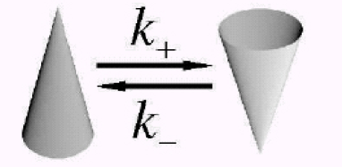
Figure 1: The two membrane components $A$ (left) and $B$ (right) have opposite cone shapes. We arbitrarily choose a positive curvature for $A$ and a negative one for $B$. A reaction interconverts both species with $k_{+}$ and $k_{-}$ being the forward and backward reaction rates, respectively.

Within this framework, we are basically interested in two situations. On the one hand, for immiscible components, we show that phase separation in the membrane leads to the spontaneous development of structures involving heterogeneous distributions of both composition and curvature that finally result in stationary finite-sized nonequilibrium domains. This instability is studied by performing a linear stability analysis of the kinetic equations, and the pattern-selection role of the reactive process is established. Corresponding numerical simulations will be shown to support these predictions. On the other hand, for miscible components we derive the correlation function for the membrane shape fluctuations. The fluctuation spectrum is mainly determined by the bending energy at small surface tension, and here we find the same expression for nonreactive and reactive cases, but with different bending rigidities. This change in the behavior of the fluctuation spectrum between equilibrium and nonequilibrium states might be easily controlled and observed in micropipet aspiration experiments.

This paper is organized as follows. In Sec. II the study of membranes of immiscible components is addressed. We propose a free energy functional, derive the kinetic equations, and perform the linear stability analysis of these equations. Numerical simulations are carried out and some representative results are shown. In Sec. III bilayers of miscible components are analyzed and the change of the height fluctuation spectrum between the reactive and nonreactive situations is established. We conclude with a brief summary in Sec. IV.

II Membranes of immiscible components

II.1 Model and analytical results

The membrane is defined as a two dimensional surface with a concentration difference order parameter $\phi$ and a local extrinsic curvature $H$. The rigidity of the membrane leads to an elastic energy contribution $\frac{\kappa}{2}\int{\left(H-H_{sp}(\phi)\right)^{2}}dxdy$ to the total energy, where $\kappa$ is the bending rigidity modulus, and the spontaneous (equilibrium) curvature $H_{sp}(\phi)$ reflects the shape asymmetry between the two lipid components. For simplicity, we adopt a linear dependence on $\phi$, $H_{sp}=\phi H_{0}$, with $H_{0}>0$ according to the schematic in Fig. 1. In the Monge parametrization geom a deformable surface is described by $(x,y,h(x,y))$, where $h(x,y)$ is the displacement (height) field for the local separation from the flat conformation. This representation is valid for surfaces that are nearly flat with only gradual variations of $h$, and allows the approximation $H\approx\nabla^{2}h$. As a function of these variables, the proposed energy functional reads

$${\mathcal{F}}=\int\left[-\frac{\alpha}{2}\phi^{2}+\frac{\beta}{4}\phi^{4}+\frac{\gamma}{2}|{\mathbf{\nabla}}\phi|^{2}+\frac{\kappa}{2}(\nabla^{2}h-\phi H_{0})^{2}\right]dxdy,$$ (1)

where the first three terms correspond to the typical Ginzburg-Landau expansion responsible for phase separation ($\alpha$, $\beta$, $\gamma>0$), with an equilibrium concentration difference $\phi_{eq}=\pm\sqrt{\alpha/\beta}$, and a typical interface length $\zeta=\sqrt{\gamma/\alpha}$. For self-assembled free membranes, the surface tension contribution ($\frac{\sigma}{2}|{\mathbf{\nabla}}h|^{2}$) in the free energy can be neglected, and we have not included it in Eq. (1).

The kinetics of $\phi$ follows a conserved scheme sancho plus the reaction contributions,

$$\frac{\partial\phi}{\partial t}=D\nabla^{2}\left[\frac{\partial{\mathcal{F}}}{\partial\phi}\right]-\Gamma(\phi-\phi_{0}),$$ (2)

where $\Gamma=k_{+}+k_{-}$ and $\phi_{0}=(k_{-}-k_{+})/(k_{+}+k_{-})$. $k_{+}$ and $k_{-}$ are the forward and backward reaction rate constants, respectively. Considering a permeable membrane (i.e., ignoring hydrodynamic interactions) we adopt the following relaxational equation for the evolution of the height field,

$$\frac{\partial h}{\partial t}=-\Lambda\frac{\delta{\mathcal{F}}}{\delta h},$$ (3)

where $\Lambda$ is a mobility parameter proportional to the inverse of the typical relaxation time $\tau_{h}$.

The kinetic equations can readily be adimensionalized: energy is measured in units of $k_{B}T$, time in units of $\tau_{h}$, and length in units of $\sqrt{D\tau_{h}}$. In terms of the new dimensionless parameters, the kinetic equations become

$$\frac{\partial\phi}{\partial t} = (\kappa H_{0}^{2}-\alpha)\nabla^{2}\phi+3\beta\phi^{2}\nabla^{2}\phi+6\beta\phi|{\mathbf{\nabla}}\phi|^{2}$$ (4)

$$~{}~{}-\gamma\nabla^{4}\phi-\kappa H_{0}\nabla^{4}h-\Gamma\left(\phi-\phi_{0}\right),$$

$$\frac{\partial h}{\partial t} = -\kappa\nabla^{4}h+\kappa H_{0}\nabla^{2}\phi.$$

At thermal equilibrium Eqs. (4) describe the spinodal decomposition of two immiscible components. Due to the composition/curvature coupling $H_{0}$, both fields will form complementary patterns. As phase segregation progresses, membrane regions with positive (negative) $\phi$ deform in such a way that the curvature become positive (negative), as shown in Fig. 2. In the absence of reaction, this coarsening process does not end until there is complete segregation into two large domains. A nonequilibrium reaction such as the one we propose converts one species into the other. This amounts to a large-scale mixing mechanism that counteracts the short-scale ordering effect of phase separation. Therefore, the segregated structures grow only until mixing and ordering effects compensate, resulting in a stationary pattern. These types of nonequilibrium patterns are also found in other systems such as polymer blends patsel ; tcong1 as well as in monomolecular adsorbtion on metal surfaces dewell ; mexPRE , and have to be distinguished from typical Turing patterns turing . Even though they emerge from the same kind of instablity (see below), Turing patterns are expected in systems with species with different diffusivities. In the model presented here, the domains result from the competition between a local thermodynamic affinity of equal species and a nonequilibrium reaction mixing effect. As we will see, linear stability analysis and numerical simulations support this idea.

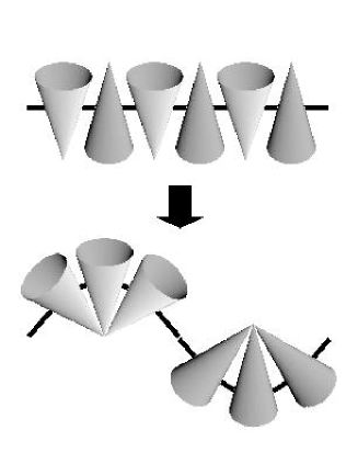
Figure 2: Schematic representation of the composition/curvature coupling effect in an unstable membrane.

The stationary uniform state corresponds to $\overline{\phi}=\phi_{0}$ and arbitrary $\overline{h}$. The linear stability of these uniform solutions is tested by adding small plane-wave perturbations of wave numer $q$ and linearizing Eqs. (4). This procedure determines the $2\times 2$ linearization matrix ${\mathcal{L}}$, with the following coefficients,

$$\begin{split}{\mathcal{L}}_{11}&=-q^{2}\left[\left(\kappa H_{0}^{2}-\alpha+3\beta\phi_{0}^{2}\right)+\gamma q^{2}\right]-\Gamma\\ {\mathcal{L}}_{12}&=-\kappa H_{0}q^{4}\\ {\mathcal{L}}_{21}&=-\kappa H_{0}q^{2}\\ {\mathcal{L}}_{22}&=-\kappa q^{4}.\end{split}$$ (5)

The eigenvalues $\omega_{q}$ of the Jacobian associated with the matrix ${\mathcal{L}}$ correspond to the linear growth rates of the perturbations. Solving the eigenvalue problem we obtain $\omega_{q}=\frac{1}{2}\left(Tr[{\mathcal{L}}]\pm\sqrt{\Delta[{\mathcal{L}}]}\right)$, where $\Delta[{\mathcal{L}}]=Tr[{\mathcal{L}}]^{2}-4Det[{\mathcal{L}}]$. At the instability boundary, $Re(\omega_{q})$ vanishes for one finite wave number that is defined as the first unstable mode. If the imaginary part of $\omega_{q}$ is not zero at this wave number, we have a wave bifurcation. The condition for this bifurcation is obtained by requiring $Tr[{\mathcal{L}}]=0$ and $\Delta[{\mathcal{L}}]<0$. For positive $\kappa$, $\Gamma$, $\alpha$, $\beta$ and $\gamma$, these conditions do not apply at any real wave number, and consequently, wave instability is not found in this model.

On the other hand, if the imaginary part of the growth rate is zero at the bifurcation point, we have a Turing-like bifurcation. The condition for this bifurcation is $Det[{\mathcal{L}}]=0$, whose analytical expression is easily obtained, yielding the following condition for the model parameters,

$$\Gamma=\Gamma_{c}\equiv\frac{\left(\alpha-3\beta\phi_{0}^{2}\right)^{2}}{4\gamma},$$ (6)

and for the wave vector of the first unstable mode,

$$q^{2}_{c}=\frac{\alpha-3\beta\phi_{0}^{2}}{2\gamma}=\sqrt{\frac{\Gamma_{c}}{\gamma}}.$$ (7)

A phase diagram is shown in Fig. 3. In the unstable region, Turing-like patterns emerging from the competition between phase separation and reaction are predicted. In the stable phase, although the two components are not inherently miscible, the reaction completely mixes the system, and the bilayer becomes stable and essentially flat.

Figure 3: Phase diagram for the case of immiscible components in the plane $(\alpha,\Gamma)$ for $\gamma=1$ and $\phi_{0}=0$. The region $\alpha<0$ (not shown) corresponds to a membrane of miscible constituents displaying a flat shape.

In the unstable phase, $\Gamma<\Gamma_{c}$, there is a range of unstable modes. Comparing with the equilibrium case ($\Gamma=0$) where a continuous range of modes starting at $q=0$ is unstable, reaction stabilizes the long wavelength modes so that, as we anticipate, the long time distribution of the system results in a stationary nonequilibrium pattern with a finite size (see further discussion in Sec. II.2). Notice in Fig. 4 that increasing $\Gamma$ reduces the range of unstable modes progressively until $\Gamma$ reaches the marginal value in Eq. (6), above which there is no longer any instability. The limits of the range of unstable modes are given by

$$q^{2}_{\pm}=\frac{\alpha-3\beta\phi_{0}^{2}}{2\gamma}\pm\frac{1}{2\gamma}\sqrt{(\alpha-3\beta\phi_{0}^{2})^{2}-4\gamma\Gamma},$$ (8)

which are independent of curvature parameters. Curvature reduces the unstable mode growth rates (see line with circles in Fig. 4) but without changing either $q_{\pm}$ or the marginal condition (6). The effect of curvature is exclusively related to the kinetics of the phase separation process (see below).

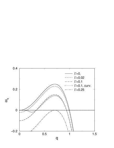
Figure 4: Dispersion relation functions $\omega_{q}$ at different values of $\Gamma$. The other parameters are held fixed at $\alpha=\gamma=1$, $\phi_{0}=0$ and $\kappa=H_{0}=0$, except for the curve with circle symbols (labeled with ‘& curv’ in the legends) that corresponds to $\kappa=10$ and $H_{0}=0.2$.

Before numerically solving the kinetic equation, we can seed light on the expected pattern formation process by performing a weakly nonlinear analysis using the amplitude equations technique. This analysis allows us to compute a solution for our problem near the bifurcation threshold, find the universality class of the pattern formation mechanism, and explain some properties such as the spatial arrangement of the patterns found in the numerical simulations.

For simplicity, we restrict the calculation of the amplitude equations to one spatial dimension. In spite of this restriction, we will be able to predict the kind of spatial arrangement found in two dimensions by using the universality properties of the amplitude equations. Details of the derivation of the amplitude equations are presented in the appendix. The analysis reveals that a solution for Eqs. (4) near the bifurcation to pattern formation reads

$$\phi\left(x,t\right) =\phi_{0}+\left[A\exp\left(iq_{c}x\right)+c.c.\right]\text{,}$$

$$h\left(x,t\right) =\overline{h}+\left[B\exp\left(iq_{c}x\right)+c.c.\right]\text{,}$$

where $c.c.$ stands for the complex conjugate, and the amplitudes $A$ and $B$ satisfy the equations

$$\begin{split}\partial_{t}A&=\left(\Gamma_{c}-\Gamma\right)A\left[1-\frac{2\beta\left(3\alpha+7\beta\phi_{0}^{2}\right)}{\left(\alpha-3\beta\phi_{0}^{2}\right)^{2}}\left|A\right|^{2}\right]+2\left(\alpha-3\beta\phi_{0}^{2}+\frac{H_{0}^{2}\kappa}{2}\right)\partial_{xx}A+\frac{3H_{0}\kappa\left(\alpha-3\beta\phi_{0}^{2}\right)}{\gamma}\partial_{xx}B\text{,}\\ \partial_{t}B&=H_{0}\kappa\partial_{xx}A+\frac{3\kappa\left(\alpha-3\beta\phi_{0}^{2}\right)}{\gamma}\partial_{xx}B\text{.}\end{split}$$ (9)

Moreover, since $B$ is purely relaxational, we can adiabatically eliminate it and reduce (9) to a single evolution equation for the amplitude $A$,

$$\begin{split}\partial_{t}A&=\left(\Gamma_{c}-\Gamma\right)A\left[1-\frac{2\beta\left(3\alpha+7\beta\phi_{0}^{2}\right)}{\left(\alpha-3\beta\phi_{0}^{2}\right)^{2}}\left|A\right|^{2}\right]+4\gamma q_{c}^{2}\partial_{xx}A\text{,}\\ B&=-\frac{H_{0}}{6q_{c}^{2}}A\text{.}\end{split}$$ (10)

Therefore, the amplitudes satisfy the real Ginzburg-Landau equation. If $\Gamma>\Gamma_{c}$ then the amplitudes relax to zero and a homogeneous state ($\phi=\phi_{0}$ and arbitrary $h=\overline{h}$) is obtained. However, if $\Gamma<\Gamma_{c}$ then the amplitudes reach a stationary value and a pattern develops if $q_{c}\in\mathbb{R}$. Notice that the amplitudes present a negative-positive aspect, that is, at sites where $A$ reaches a maximum (minimum) $B$ reaches a minimum (maximum). This is simply a consequence of the particular selection of sign for the spontaneous curvature $H_{0}$. With regard to the nonlinear term, $A\left|A\right|^{2}$, note first that its coefficient is always negative. As a result, the nonlinearity always plays a stabilizing role, the bifurcation to pattern formation is supercritical for all values of the parameters, and no hysteresis may occur. Secondly, the nonlinear term provides information about the relevant modal interactions. At this point, we can take advantage of the universality properties of the amplitude equations to infer the spatial arrangement of the pattern in two dimensions. Since the Swift-Hohenberg model also shares the same universality class when performing an amplitude equation analysis, namely, it also reduces to the real Ginzburg-Landau equation hecke ; newell , the pattern formation mechanism is the same in both models. It is well-known in that case that the modal interactions in two dimensions are such that if the inversion symmetry is preserved then roll-like patterns develop. On the other hand, if that symmetry is not fulfilled, a hexagonal structure appears. Note that in Eqs. (4) the inversion symmetry, $\{\phi\rightarrow-\phi,h\rightarrow-h\}$ is only satisfied if $\phi_{0}=0$. Thus we expect a roll-like pattern in that case, while hexagons will develop otherwise.

II.2 Numerical results

Numerical integration of Eqs. (4) has been performed in two dimensions using an explicit Euler scheme in a square lattice with periodic boundary condition. Small random perturbations around $\overline{\phi}=\phi_{0}$ and $\overline{h}=0$ are implemented as initial conditions. The coordinate step $\Delta x$ was chosen equal to $1$, and the time step was usually $\Delta t=10^{-4}$ to assure good numerical accuracy (length and time in dimensionless simulation units). The numerical results presented in this section correspond to highly immiscible components (deep quench, $\alpha=1$ and $\beta=1$, leading to an equilibrium value of $\phi_{eq}=\pm 1$), and an interface thickness of the order of the space discretization ($\zeta=1$, which leads to $\gamma=1$). The bending rigidity modulus is taken equal to $10$ (in units of $k_{B}T$) kapa , and we consider two constituent lipids of very different shapes by setting $H_{0}=0.2$. All our numerical results are consistent with the predictions of the linear stability analysis and the amplitude equations. Representative numerical results are presented below.

In Fig. 5 we show the simulation results for three different situations. The first row corresponds to small $\Gamma=0.05$ and a critical quench ($\phi_{0}=0$), showing the development of a laberynthine pattern that is still evolving at $t=2000$ (the longest time for the snapshots shown in the figure). The coarsening process, however, is progressively slowed down later on. The $\phi$-field profiles of these domains (horizontal cross-sectional cuts through the pattern) reveal regions where $\phi_{eq}$ is $+1$ or $-1$ connected by abrupt boundaries that indicate the short spatial range over which the equilibrium order parameter changes from one value to the other. This is a signature of the fact that the phase separation process is dominant for this value of $\Gamma$. The second and third sets of panels correspond to large $\Gamma=0.2$ (the marginal condition for the selected parameters is $\Gamma_{c}=0.25$) showing laberynthine (critical quench in the second row) and quasi-hexatic droplet-like (off critical quench, $\phi_{0}=0.1$, in the third set) patterns. A spatial Fourier transform of this stationary pattern shows a clear hexagonal structure. These domains are already stationary at times longer than $t=2000$, and can indeed be considered as nonequilibrium stable phases of the system, involving both composition and curvature modulations. Their $\phi$- and $h$-field profiles have a smooth harmonic shape due to the strength of the reactive process. In both cases, since we are close to the bifurcation boundary, small local deviations from the stationary values are obtained. We especially monitor the variations of the height field and find that $\langle|\nabla h|\rangle<0.05$ is satisfied, so that the model has a real physical correspondence.

Figure 5: Three sets of selected patterns resulting from the numerical simulation based on Eqs. (4). First row: $\Gamma=0.05$, $\phi_{0}=0$. Second row: $\Gamma=0.2$, $\phi_{0}=0$. Third row: $\Gamma=0.2$, $\phi_{0}=0.1$ (off critical quench), showing an array of droplet-like domains rich in the minority species. The first three panels in each row correspond to the $\phi$-field distributions of a $128\times 128$ system at $t=100$, $400$ and $2000$ (from left to right). Darker (lighter) regions are richer in the $A$ ($B$) lipid. In the last panel of each row the height field has been plotted in three dimensions for a $64\times 64$ portion of the corresponding system at $t=2000$. Some exaggeration along the vertical direction has been applied.

In order to assess the kinetic ordering process more quantitatively, we monitor the domain size $L(t)$ computed from the composition correlation functions $\langle\phi({\bf r^{\prime}},t)\phi({\bf r^{\prime}}+{\bf r},t)\rangle$ (the same results are obtained using the height correlation functions). Here, the brackets $\langle\cdots\rangle$ indicate not only an average over orientations of ${\bf r}$ and over surface positions ${\bf r^{\prime}}$, but also over different realizations of random initial conditions. As has been reported in other studies, curvature considerably slows down the coarsening segregation process. This is specially evident when reaction is absent, and for this situation different kinetic approaches have been invoked. A mean-field kinetic scheme by Taniguchi dyn3 leads to extremely slow laberynthine stripe growth obeying $L(t)\sim t^{r}$ with $r=0.1$, instead of the usual spinodal decomposition growth exponent of $1/3$ lifs . Later, Monte Carlo simulations dyn2 ; dyn1 showed how, in the long time evolution, those stripes break up into disconnected buds that subsequently diffuse and coalesce. In our model, when the reactive term is removed, similar results as those presented in Ref. dyn3 are obtained, and no stripe breakup is observed. The reason for the disagreement between the analytic and Monte Carlo schemes is probably due to the fact that continuum models subjected to a specific parametrization of the surface such as given in Eqs. (4) do not allow for overhangs that are surely crucial in the late stages of membrane phase segregation.

However, the cases in which there is no reaction or in which the reaction is weak are not of interest for us, since in these cases the system evolves in such away that large gradients of the height displacement field occur. As noted above, when this happens the Monge surface parametrization is not valid and the model, although mathematically robust, does not describe the physical behavior of any real system. In the reactive cases, however, the slow kinetics is still observed for the times prior to stationary pattern formation. This is observed in Fig. 6, where a set of curves showing the domain size $L(t)$ is presented for several values of $\Gamma$. The situations with and without curvature are compared for each case. Notice how the deformable systems evolve more slowly than the nondeformable ones, although the same final stationary size is achieved. There is no theory to explain such a slowing down effect, but some hand-waving arguments may explain the physical reasons for this behavior. Monitoring of the different energy contributions in Eq. (1) indicates that at early times (when the kinetics with and without curvature are still quite similar) interfacial energy due to the rapid formation of composition domains is much larger than any other energy contribution. In other words, phase separation proceeds and membrane curvature follows the composition change. At this stage the reduction of the interfacial energy governs the coarsening process, leading to the $1/3$ Lifshitz-Slyozov exponent. Later, at intermediate times, when composition domains become larger, the height order parameter is no longer able to keep up with the phase separation process and some curvature energy is stored, causing the whole coarsening process to slow down.

Figure 6: Log-log plots of $L(t)$ vs $t$ for different values of $\Gamma$. The values of $L(t)$ have been computed as an average over $10$ runs of the correlation functions in $128\times 128$ systems. In all cases $\phi_{0}=0$. The curvature parameters are set to $\kappa=10$, $H_{0}=0.2$ for the thin lines, and $\kappa=H_{0}=0$ for the thicker lines.

The final size of the nonequilibrium stationary domains, $L_{f}=L(t\rightarrow\infty)$, is determined by the reaction parameter. The dependence of the final pattern size on the reaction parameter, $L_{f}\sim\Gamma^{-s}$, has been largely discussed in the literature patsel ; chri ; liu . The results of our model also reproduce the two limiting behaviors: $s=1/4$ for large $\Gamma$ (close to its marginal value), and $s=1/3$ for small $\Gamma$. In Fig. 7, $L_{f}$ is plotted for different values of the reaction parameter. Linear fits for the four first and the last four data points give the slopes $0.323\pm 0.006$ and $0.26\pm 0.006$, respectively. The derivation of the exponent values for the rigid situation (nondeformable surfaces) is performed by minimizing an effective free energy expression (where the reactive term is included via Green’s functions) in a square (small $\Gamma$) and a harmonic (large $\Gamma$) approximation for the stationary concentration field chri ; liu . In the present model, the curvature kinetics relaxationally follows the concentration dynamics. At longer times (when the stationary patterns are already achieved) no significant curvature energy is present in the system, so that we can neglect the curvature contributions in Eq. (1) and the results in Refs. chri ; liu are recovered.

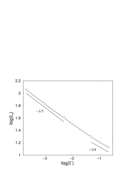
Figure 7: Log-log plot of $L_{f}$ vs. $\Gamma$. The slopes $1/4$ and $1/3$ are plotted for comparison with the large and small $\Gamma$ regimes, respectively. All the points have been calculated for $\phi_{0}=0$, $\kappa=10$ and $H_{0}=0.2$, at sufficiently long times to consider the growth process practically halted. We have performed an average over $10$ realizations. The system sizes are $128\times 128$ for large $\Gamma$, and $256\times 256$ for small $\Gamma$.

In Eq. (3) we ignored the hydrodynamic effects due to the background fluid velocity by considering a permeable membrane through which the fluid drains freely as the system evolves. Solvent hydrodynamic effects seif can be approached through a renormalized height mobility $\Lambda=\left(4\mu q\right)^{-1}$ in the second of Eqs. (4) in Fourier space, where $\mu$ is the solvent kinematic viscosity. The inclusion of this $q$-dependent mobility does not change the main results of the stability analysis and numerical simulations shown so far.

Before ending this section, we check the applicability of our results to real membrane systems. We adimensionalized the kinetic equations to units in which $D=\Lambda=k_{B}T=1$. Redimensionalizing them, taking the typical values $D=10^{-7}-10^{-8}$cm²/s (for lipids in a liquid-phase membrane), $\mu=1$cp ($H_{2}O$ at $20^{\circ}$C) and the typical unstable modes $q\approx q_{c}=0.5$, we find that the size of the patterns obtained above lies within the range $2-20\mu$m, which is accessible in giant vesicle ($10-100\mu$m in diameter) experiments.

III Membranes of miscible components: Linearization and shape fluctuations

In this section we consider a parameter region where the membrane is thermodinamically stable. The instability in the previous section was caused by the immiscibility of the two lipid components, while we now consider the case of miscible membrane constituents. Notice that the two situations could correspond to the same physical system but at different temperatures, below (unstable) or above (stable) the critical temperature. For the stable case we adopt the following free energy functional,

$${\mathcal{F}}=\int\left[-\frac{\alpha}{2}\phi^{2}+\frac{\kappa}{2}(\nabla^{2}h-\phi H_{0})^{2}+\frac{\sigma}{2}\left(|{\mathbf{\nabla}}h|\right)^{2}\right]dxdy,$$ (11)

where $\alpha$ is now negative, and the nonlinear ($\beta$) and line tension ($\gamma$) terms have been removed since they are irrelevant in the absence of phase segregation. An additional surface tension term has been included in order to study membranes under tension.

In the equilibrium situation (no reaction), the concentration field can be integrated out ($\frac{\partial{\mathcal{F}}}{\partial\phi}=0$) from Eq. (11), leading to $\phi_{eq}=\frac{\kappa H_{0}}{\kappa H_{0}^{2}-\alpha}\nabla^{2}h$. Inserting $\phi_{eq}$ in Eq. (11) we obtain an effective free energy for $h$ alone,

$${\mathcal{F}}_{eff}=\int\left[\frac{\kappa_{eff}}{2}(\nabla^{2}h)^{2}+\frac{\sigma}{2}\left(|{\mathbf{\nabla}}h|\right)^{2}\right]dxdy,$$ (12)

with an effective rigidity modulus andel

$$\kappa_{eff}=\kappa\left[1-\left(\frac{\kappa H_{0}^{2}}{\kappa H_{0}^{2}-\alpha}\right)\right].$$ (13)

Notice that, as a consequence of the composition/curvature coupling, the different preferred curvature of the lipid components acts to reduce the rigidity modulus from $\kappa$ to $\kappa_{eff}$. Note also that $\kappa_{eff}>0$ for negative values of $\alpha$, so that the stability of the membrane is assured above the critical temperature.

The dynamics for the immiscibility situation has so far been considered to be strictly deterministic. Here, however, in order to obtain dynamical steady state functions, we add stochastic forces to the kinetic equations and perform an average over an appropriate ensemble. The dimensionless kinetic equation for $\phi$, once the reactive terms are included, reads

$$\frac{\partial\phi}{\partial t}=\nabla^{2}\left[\frac{\partial{\mathcal{F}}}{\partial\phi}\right]-\Gamma(\phi-\phi_{0})+{\mathbf{\nabla}}\cdot{\bf f}_{\phi},$$ (14)

where the last term corresponds to a conserving Gaussian noise with correlations $\langle f_{\phi}({\bf r},t)f_{\phi}({\bf r^{\prime}},t^{\prime})\rangle=2k_{B}T\delta({\bf r}-{\bf r^{\prime}})\delta(t-t^{\prime})$. For the curvature order parameter we again adopt the relaxational equation for a permeable surface,

$$\frac{\partial h}{\partial t}=-\Lambda\frac{\delta{\mathcal{F}}}{\delta h}+f_{h},$$ (15)

with $\Lambda=1$ in dimensionless units, and $f_{h}$ is a thermal equilibrium noise with correlations $\langle f_{h}({\bf r},t)f_{h}({\bf r^{\prime}},t^{\prime})\rangle=2k_{B}T\delta({\bf r}-{\bf r^{\prime}})\delta(t-t^{\prime})$.

The kinetic equations become

$$\begin{split}\frac{\partial\phi}{\partial t}=(\kappa H_{0}^{2}-\alpha)\nabla^{2}\phi-\kappa H_{0}\nabla^{4}h-\Gamma\left(\phi-\phi_{0}\right)+{\mathbf{\nabla}}\cdot{\bf f}_{\phi}\\ \frac{\partial h}{\partial t}=-\kappa\nabla^{4}h-\sigma\nabla^{2}h+\kappa H_{0}\nabla^{2}\phi+f_{h}.\end{split}$$ (16)

The important quantity to characterize membrane shape fluctuations is the height variance $\langle|h_{q}|^{2}\rangle$ at wave number $q$, which is calculated by linearizing the kinetic equations (16) and solving them in Fourier space. If $\hat{\phi}({\bf q},\omega)$ and $\hat{h}({\bf q},\omega)$ are the Fourier transforms of $\phi({\bf r},t)$ and $h({\bf r},t)$, respectively, Eqs. (16) can be written as

$$i\omega\left(\begin{tabular}[]{c}$\hat{\phi}({\bf q},\omega)$\\ $\hat{h}({\bf q},\omega)$\end{tabular}\right)=\left(\begin{tabular}[]{cc}$a_{11}$&$a_{12}$\\ $a_{21}$&$a_{22}$\end{tabular}\right)\times\left(\begin{tabular}[]{c}$\hat{\phi}({\bf q},\omega)$\\ $\hat{h}({\bf q},\omega)$\end{tabular}\right)+\left(\begin{tabular}[]{c}$i{\bf q}\cdot{\bf f}_{\phi}$\\ $f_{h}$\end{tabular}\right),$$ (17)

where

$$\begin{split}a_{11}&=-\left(\kappa H_{0}^{2}-\alpha\right)q^{2}-\Gamma\\ a_{12}&=-\kappa H_{0}q^{4}\\ a_{21}&=-\kappa H_{0}q^{2}\\ a_{22}&=-\kappa q^{4}+\sigma q^{2}\,.\end{split}$$ (18)

Solving these coupled equations, and using the statistical properties of the thermal noises, yields

$$\langle\hat{h}(q,\omega)\hat{h}^{*}(q,\omega)\rangle=\frac{2k_{B}T\left(a_{21}^{2}q^{2}+\omega^{2}+a_{11}^{2}\right)}{\omega^{2}\left(a_{11}+a_{22}\right)^{2}+\left(a_{12}a_{21}-a_{11}a_{22}+\omega^{2}\right)^{2}}.$$ (19)

On integrating over $\omega$, the height variance follows the general expression,

$$\langle|h_{q}|^{2}\rangle=\frac{1}{\nu-\eta}\left[\frac{A}{\sqrt{\nu\eta}}+A^{\prime}\right]\left[\sqrt{-\eta}-\sqrt{-\nu}\right],$$ (20)

where $\nu$ and $\eta$ are negative variables that read

$$\left(\begin{tabular}[]{c}$\nu$\\ $\eta$\end{tabular}\right)=-\frac{B}{2}\pm\frac{1}{2}\sqrt{B^{2}-4C},$$ (23)

and

$$\begin{split}A&=2k_{B}T\left(a_{21}^{2}q^{2}+a_{11}^{2}\right)\\ A^{\prime}&=2k_{B}T\\ B&=a_{11}^{2}+a_{22}^{2}+2a_{21}a_{12}\\ C&=\left(a_{11}a_{22}-a_{21}a_{12}\right)^{2}.\end{split}$$ (24)

In the absence of the reaction, the evaluation of Eq. (20) in the long-wavelength limit for a tensionless membrane leads to $\langle|h_{q}|^{2}\rangle=k_{B}T/\kappa_{eff}q^{4}$. This behavior is truncated and replaced by $k_{B}T/\sigma q^{2}$ for a membrane under tension if only the dominant terms at small $q$ are retained. Keeping the dominant and the first subdominant terms, one recovers the well known expression for the height variance in an equilibrium membrane,

$$\langle|h_{q}|^{2}\rangle=\frac{k_{B}T}{\sigma q^{2}+\kappa_{eff}q^{4}}.$$ (25)

Notice that this result is obtained in a much simpler way from an equilibrium average using the effective free energy in Eq. (12).

One of the usual experiments to study equilibrium membrane shape fluctuations is based on the micropipet aspiration technique evans . In these experiments, a pressure difference is applied inside a micropipet in contact with a vesicle membrane. This creates a tension in the membrane that pulls the excess area $\Delta S$ due to the thermal shape fluctuations inside the micropipet. By means of this technique, the areal strain $\bar{\alpha}\equiv\Delta S/S$ is obtained experimentally for different values of the applied tension $\sigma$. According to Eq. (25), the relative areal strain $\Delta\bar{\alpha}\equiv\bar{\alpha}-\bar{\alpha}_{0}$ ($\bar{\alpha}_{0}$ being the areal strain for a reference value $\sigma_{0}$) can be calculated analytically nuovo ; fournier :

$$\Delta\bar{\alpha}=\frac{k_{B}T}{8\pi\kappa_{eff}}\ln\left(\frac{\sigma}{\sigma_{0}}\right).$$ (26)

Therefore, the slope of the logarithm of $\sigma$ versus $\Delta\bar{\alpha}$ obtained by the micropipet technique yields a measure of the effective bending modulus. Note that in these experiments a certain tension $\sigma$ is needed, but it has to be small since otherwise the $\kappa_{eff}q^{4}$ term in Eq. (25) would be insignificant compared to $\sigma q^{2}$.

Now the question is, how is the shape fluctuation spectrum affected by the presence of the reaction? In other words, how would the nonequilibrium membranes described here behave in micropipet experiments? To answer this, we evaluate Eq. (20) for $\Gamma\neq 0$ and keep only the dominant terms in the limit $q\rightarrow 0$. For tensionless membranes we get $\langle|h_{q}|^{2}\rangle=k_{B}T/\kappa q^{4}$ and for membranes under tension we recover $\langle|h_{q}|^{2}\rangle=k_{B}T/\sigma q^{2}$. Keeping the dominant terms for both limits, in the weak tension regime the fluctuation spectrum reads

$$\langle|h_{q}|^{2}\rangle=\frac{k_{B}T}{\sigma q^{2}+\kappa q^{4}}.$$ (27)

Comparing this result with the fluctuation spectrum obtained for membranes with active proteins prost3 ; sum ; prost4 , no novel nonequilibrium contribution to the height fluctuations is found here. The effect of the nonequilibrium reaction in stable membranes results in a change between a regime governed by $\kappa_{eff}$ to another one with the actual rigidity $\kappa$. Thus, the reaction makes the membrane more rigid by simply removing the composition/curvature coupling effect that diminished the rigidity in the equilibrium situation. This change is more evident when the two components of the bilayer are rather different in shape and miscible but close to the critical temperature. In this situation (large $H_{0}$ and $\bar{\alpha}\lesssim 0$) the difference between $\kappa$ and $\kappa_{eff}$ might be experimentally observable.

Some caution, however, must be observed when deriving Eq. (27). In order to evaluate Eq. (20) for small $q$, we considered the terms $\Gamma^{2}$ to be dominant with respect to the terms $2\Gamma\left(\kappa H_{0}^{2}-\alpha\right)q^{2}$ (subdominant) and also with respect to the subsubdominant quartic contributions $\left(\sigma+\left(\kappa H_{0}^{2}-\alpha\right)\right)q^{4}$ (which are those that led to Eq. (25)). However, the analysis becomes more difficult if one notices that we are not in the region of asymptotically small wavenumbers since the smallest $q$ accessible to an experiment is of order $1/L$, where $L$ is the linear system size. Thus, one must look in detail at the values of the parameters in order to determine exactly which terms initially considered subdominant might indeed be dominant when the reaction is present. $\Gamma^{2}$ is dominant if $\Gamma>2\left(\kappa H_{0}^{2}-\alpha\right)q_{min}^{2}$, with $q_{min}\sim 1/L$ and thus dependent on the system size. We know that for a sufficiently strong reactive process, $\Gamma^{2}$ dominates and Eq. (27) holds, but for intermediate values of $\Gamma$ the spectrum could change significatively. When $2\Gamma\left(\kappa H_{0}^{2}-\alpha\right)q^{2}$ becomes dominant, $\langle|h_{q}|^{2}\rangle=\frac{k_{B}T}{\left(\Gamma\kappa/\sqrt{8\Gamma\left(\kappa H_{0}^{2}-\alpha\right)}\right)q^{3}}$ for a tensionless membrane. These regimes are captured in Fig. 8, where a set of $\langle|h_{q}|^{2}\rangle$ curves is plotted for $\sigma=0$. Very large and zero values for $\Gamma$ show the $q^{-4}$ behavior, although with different rigidity factors ($\kappa$ and $\kappa_{eff}$, respectively). At intermediate $\Gamma$, the $q^{-3}$ behavior appears as predicted above.

Figure 8: Log-log plot for $\langle|h_{q}|^{2}\rangle$ evaluated from Eq. (20) in a tensionless membrane for different values of $\Gamma$. The other parameters are $\alpha=-0.01$, $\kappa=10$ and $H_{0}=0.2$ ($\kappa_{eff}=2$ in these cases). The slopes $-1/4$ and $-1/3$ are plotted to identify the different regimes.

The inclusion of hydrodynamic interactions can again be accomplished by considering $\Lambda=\left(4\mu q\right)^{-1}$ in the Fourier transform of Eq. (15). This modifies the coefficients $a_{21}$ and $a_{22}$ in Eq. (18), which are now divided by $\left(4\mu q\right)$. Accordingly, the $f_{h}$ thermal noise correlations also change to $\langle f_{h}({\bf r},t)f_{h}({\bf r^{\prime}},t^{\prime})\rangle=\frac{2k_{B}T}{\left(4\mu q\right)}\delta({\bf r}-{\bf r^{\prime}})\delta(t-t^{\prime})$, and therefore the parameter $A^{\prime}$ in Eq. (24) has to be divided by $\left(4\mu q\right)$ as well. However, with these modifications the evaluation of $\langle|h_{q}|^{2}\rangle$ again leads to the results in Eqs. (25) and (27).

IV Conclusions

Starting with a simple model of a deformable reactive membrane composed of two differently shaped molecules, we show that stationary finite-sized patterns may appear under some parameter conditions for the immiscibility situation as a result of the competition between phase segregation and reaction. These structures involve heterogeneous distributions of composition and curvature whose sizes are determined by the nonequilibrium reactive process. For typical values of the viscosity of water and lipid lateral diffusion constants in bilayers, and at normal room temperatures, such patterns are predicted to have a size of a few microns (see the discussion at the end of Sec. II.2). Therefore, this behavior would correspond to a reliable pattern formation mechanism in lipid membranes which we believe to be experimentally accessible in giant synthetic vesicles. The amplitude of these patterns is modulated by the bilayer rigidity and the spontaneous curvature of its components. In our numerical calculations we have used realistic typical values for the rigidity, while the spontaneous curvature depends on the specific geometry of the membrane constituents. We specifically propose that azobenzene compounds, which are known to show amphiphilic behavior in Langmuir monolayers, and whose shapes are strongly modified by means of well-known photoisomerization reactions rau ; our , might be suitable to test our predictions. The selection of the applied light wavelength and its intensity may determine both the fraction of the two isomers ($\phi_{0}$) and the strength of the reactive process ($\Gamma$), respectively. Thus, experimental work on synthetic vesicle membranes made of these compounds can be specifically designed to confirm the results of this model.

In the same context, for miscible components membranes we have found a difference between the equilibrium and nonequilibrium situations. The effects of the composition/curvature coupling and the reactive process on the membrane rigidity are established. Micropipet experiments with the proposed membrane systems might confirm these results.

Appendix A Derivation of the amplitude equations

The starting point of the analysis is the one dimensional version of the model for reactive membranes presented herein,

$$\varphi_{t} =\left(\kappa H_{0}^{2}-\alpha\right)\varphi_{xx}+3\beta\left(\varphi+\phi_{0}\right)^{2}\varphi_{xx}+6\beta\left(\varphi+\phi_{0}\right)\left(\varphi_{x}\right)^{2}-\gamma\varphi_{xxxx}$$

$$-\kappa H_{0}h_{xxxx}-\frac{\left(\alpha-3\beta\phi_{0}^{2}\right)^{2}}{4\gamma}\left(1-\varepsilon\right)\varphi\text{,}$$ (28)

$$h_{t} =-\kappa h_{xxxx}+\kappa H_{0}\varphi_{xx}\text{.}$$

For convenience, we have introduced in Eqs. (28) some notation changes and definitions with respect to the ones that appear in Eqs. (4). Thus, in Eqs. (28) subscripts indicate partial derivatives, the field $\varphi=\phi-\phi_{0}$ has been defined, and we have introduced the control parameter $\varepsilon=\left(\Gamma_{c}-\Gamma\right)/\Gamma_{c}$ that accounts for the “distance” to the bifurcation between a homogenous state ($\varepsilon<0$) and pattern formation ($\varepsilon>0$). The homogeneous state according to this definitions corresponds to $\varphi=0$ and arbitrary $h=\overline{h}$.

As shown in Sec. (II.1), by linearizing Eqs. (28) one can easily check that if $\varepsilon>0$ then the homogeneous state becomes unstable and,

$$\begin{split}\varphi\left(x\right)&=A\exp\left(iq_{c}x\right)+A^{\ast}\exp\left(-iq_{c}x\right)\text{,}\\ h\left(x\right)&=B\exp\left(iq_{c}x\right)+B^{\ast}\exp\left(-iq_{c}x\right)\text{,}\end{split}$$ (29)

is a solution in the steady state if $q_{c}^{2}=\left(\alpha-3\beta\phi_{0}^{2}\right)/\left(2\gamma\right)$. It is worth noting that in Eqs. (29) we have arbitrarily taken $\overline{h}=0$ without any loss of generality. Moreover, by substituting (29) into (28) and expanding up to the first harmonic, $\mathcal{O}\left(\exp\left(iq_{c}x\right)\right)$, one finds that the amplitudes scale as a function of $\varepsilon$ as $A,B\sim\sqrt{\varepsilon}$. Thus, we expect that near the bifurcation the following expansion holds,

$$\begin{split}\varphi&=\sum_{n=1}^{\infty}\varepsilon^{n/2}\varphi^{\left(n\right)}\text{,}\\ h&=\sum_{n=1}^{\infty}\varepsilon^{n/2}h^{\left(n\right)}\text{.}\end{split}$$ (30)

By computing the linear growth rate, $\omega_{q}$, that is, the largest eigenvalue of the linear problem (see Eqs. (5)), we also note that,

$$\left.\omega_{q}\right|_{\begin{subarray}{c}q\rightarrow q_{c}\\ \varepsilon\rightarrow 0\end{subarray}}\simeq C_{1}\varepsilon+C_{2}\left(q-q_{c}\right)^{2}\text{,}$$

where $C_{i}$ are constants. Thus, as a function of $\varepsilon$ the width of the band of unstable modes scales as $\sim\varepsilon^{1/2}$. Then, since all modes $\exp\left(iqx\right)$ can be written as $\exp\left(i\left(q-q_{c}\right)x\right)\exp\left(-iq_{c}x\right)$, a separation of spatial scales can be performed between the most unstable mode (fast) and the rest of the modes of the unstable band (slow). Let us call the slow modulation spatial scale $X$, such that $X=\varepsilon^{1/2}x$, where $x$ will now stand for the fast spatial scale. We also note that

$$\left.\exp\left(\omega_{q}t\right)\right|_{\begin{subarray}{c}q\rightarrow q_{c}\\ \varepsilon\rightarrow 0\end{subarray}}\simeq\exp\left(\varepsilon t\right)\text{.}$$

Therefore we can define a slow time scale as a function of the control parameter, $T=\varepsilon t$. The separation of scales can be implemented in Eqs. (28) by replacing the spatial and temporal derivatives according to the chain rule such that $\partial_{x}\rightarrow\partial_{x}+\varepsilon^{1/2}\partial_{X}$ and $\partial_{t}\rightarrow\varepsilon\partial_{T}$.

By implementing the separation of scales and substituting Eqs. (30) into Eqs. (28) we obtain a rather cumbersome expansion in terms of $\varepsilon$. The lowest order contribution is of $O\left(\varepsilon^{1/2}\right)$ and reads

$$\begin{split}\left(3\beta\phi_{0}^{2}+H_{0}^{2}\kappa-\alpha\right)\varphi_{xx}^{\left(1\right)}-\gamma\varphi_{xxxx}^{\left(1\right)}-\frac{\left(\alpha-3\beta\phi_{0}^{2}\right)^{2}}{4\gamma}\varphi^{\left(1\right)}-H_{0}\kappa h_{xxxx}^{\left(1\right)}&=0\text{,}\\ H_{0}\kappa\varphi_{xx}^{\left(1\right)}-\kappa h_{xxxx}^{\left(1\right)}&=0\text{.}\end{split}$$ (31)

Note that Eqs. (31) correspond to the linearized version of Eqs. (28) in the stationary state. We define the linear operator

$$\mathbb{L}\equiv\left(\begin{array}[c]{cc}-\frac{\left(\alpha-3\beta\phi_{0}^{2}\right)^{2}}{4\gamma}+\left(3\beta\phi_{0}^{2}+H_{0}^{2}\kappa-\alpha\right)\partial_{xx}-\gamma\partial_{xxxx}&-H_{0}\kappa\partial_{xxxx}\\ H_{0}\kappa\partial_{xx}&-\kappa\partial_{xxxx}\end{array}\right)\text{.}$$

Then, Eqs. (31) can be trivially written as $\mathbb{L}\mathbf{\chi}_{1}=0$, where $\left(\mathbf{\chi}_{n}\right)^{T}=\left(\varphi^{\left(n\right)},h^{\left(n\right)}\right)$. The contributions of the next order, $O\left(\varepsilon\right)$, are $\mathbb{L}\mathbf{\chi}_{2}=\mathbf{\psi}_{2}\left(\left\{\varphi^{\left(1\right)};h^{\left(1\right)}\right\}\right)$ where $\mathbf{\psi}_{2}^{T}=\left(\mathbf{\psi}_{2}^{\left(a\right)}\mathbf{,\psi}_{2}^{\left(b\right)}\right)$,

$$\mathbf{\psi}_{2}^{\left(a\right)} =-6\beta\phi_{0}\left(\left(\varphi_{x}^{\left(1\right)}\right)^{2}+\varphi^{\left(1\right)}\varphi_{xx}^{\left(1\right)}\right)+2\left(\alpha-3\beta\phi_{0}^{2}-H_{0}^{2}\kappa\right)\varphi_{xX}^{\left(1\right)}+$$

$$+4\gamma\varphi_{xxxX}^{\left(1\right)}+4H_{0}\kappa h_{xxxX}^{\left(1\right)}\text{,}$$

$$\mathbf{\psi}_{2}^{\left(b\right)} =2\kappa\left(-H_{0}\varphi_{xX}^{\left(1\right)}+2h_{xxxX}^{\left(1\right)}\right)\text{,}$$

Finally, at order $\varepsilon^{3/2}$ we get $\mathbb{L}\mathbf{\chi}_{3}=\mathbf{\psi}_{3}\left(\left\{\varphi^{\left(1\right)},\varphi^{\left(2\right)};h^{\left(1\right)},h^{\left(2\right)}\right\}\right)$, where $\mathbf{\psi}_{3}^{T}=\left(\mathbf{\psi}_{3}^{\left(a\right)}\mathbf{,\psi}_{3}^{\left(b\right)}\right)$ reads,

$$\mathbf{\psi}_{3}^{\left(a\right)} =\varphi_{T}^{\left(1\right)}-\Gamma_{c}\varphi^{\left(1\right)}-6\beta\varphi_{x}^{\left(1\right)}\left(\varphi^{\left(1\right)}\varphi_{x}^{\left(1\right)}+2\phi_{0}\left(\varphi_{X}^{\left(1\right)}+\varphi_{x}^{\left(2\right)}\right)\right)+$$

$$+\left(\alpha-H_{0}^{2}\kappa\right)\left(\varphi_{XX}^{\left(1\right)}+2\varphi_{xX}^{\left(2\right)}\right)-3\beta\left[\phi_{0}^{2}\left(\varphi_{XX}^{\left(1\right)}+2\varphi_{xX}^{\left(2\right)}\right)+\right.$$

$$\left.+\varphi_{xx}^{\left(1\right)}\left(\left(\varphi^{\left(1\right)}\right)^{2}+2\phi_{0}\varphi^{\left(2\right)}\right)+2\phi_{0}\varphi^{\left(1\right)}\left(2\varphi_{xX}^{\left(1\right)}+\varphi_{xx}^{\left(2\right)}\right)\right]+$$

$$+2\gamma\left(3\varphi_{xxXX}^{\left(1\right)}+2\varphi_{xxxX}^{\left(2\right)}\right)+2H_{0}\kappa\left(3h_{xxXX}^{\left(1\right)}+2h_{xxxX}^{\left(2\right)}\right)\text{,}$$

$$\mathbf{\psi}_{3}^{\left(b\right)} =h_{T}^{\left(1\right)}+\kappa\left(2\left(3h_{xxXX}^{\left(1\right)}+2h_{xxxX}^{\left(2\right)}\right)-H_{0}\left(\varphi_{XX}^{\left(1\right)}+2\varphi_{xX}^{\left(2\right)}\right)\right)\text{.}$$

We could continue up to any order with the expansion. In all cases we will obtain a nonlinear equation, such that at order $\varepsilon^{n/2}$,

$$\mathbb{L}\mathbf{\chi}_{n}=\mathbf{\psi}_{n}\left(\left\{\varphi^{\left(1\right)},\ldots,\varphi^{\left(n-1\right)};h^{\left(1\right)},\ldots,h^{\left(n-1\right)}\right\}\right)\text{.}$$ (32)

However, at order $\varepsilon^{3/2}$ we are already able to extract a closed evolution equation for the amplitudes of the pattern and so we will stop at that order.

Our task is to solve the hierarchy of equations given by (32). At order $\varepsilon^{1/2}$ the problem is homogeneous and with appropriate boundary conditions,

$$\begin{split}\varphi^{\left(1\right)}&=A\left(X,T\right)\exp\left(iq_{c}x\right)+A^{\ast}\left(X,T\right)\exp\left(-iq_{c}x\right)\text{,}\\ h^{\left(1\right)}&=B\left(X,T\right)\exp\left(iq_{c}x\right)+B^{\ast}\left(X,T\right)\exp\left(-iq_{c}x\right)\text{,}\end{split}$$ (33)

is a solution. However, the amplitudes $A$ and $B$ are undetermined at this point. The subsequent orders are no longer homogeneous and therefore their solvability can not be ensured unless one implements the so-called Fredholm alternative theorem newell . In our case the application of the theorem simply states, as a recipe, that for Eqs. (32) to have a solution the functions $\psi_{n}$ can not contain the fundamental mode $\exp\left(\pm iq_{c}x\right)$. Thus, by substituting the solution (33) into the next order or the hierarchy and imposing the solvability condition we obtain

$$\varphi^{\left(2\right)} =-\frac{8\beta\phi_{0}}{3\left(\alpha-3\beta\phi_{0}^{2}\right)}\left[\left(A\left(X,T\right)\right)^{2}\exp\left(i2q_{c}x\right)+\left(A\left(X,T\right)^{\ast}\right)^{2}\exp\left(-i2q_{c}x\right)\right]\text{,}$$

$$h^{\left(2\right)} =\frac{4\beta\phi_{0}\gamma H_{0}}{3\left(\alpha-3\beta\phi_{0}^{2}\right)^{2}}\left[\left(A\left(X,T\right)\right)^{2}\exp\left(i2q_{c}x\right)+\left(A\left(X,T\right)^{\ast}\right)^{2}\exp\left(-i2q_{c}x\right)\right]\text{.}$$

Once again, the value of $A$ and $B$ can not be determined at this order. However, at order $\varepsilon^{3/2}$ the application of the Fredholm theorem provides the conditions that determine the values of the amplitudes $A$, $B$. These conditions constitute the amplitude equations for our pattern forming system,

$$\partial_{T}A =\frac{\left(\alpha-3\beta\phi_{0}^{2}\right)^{2}}{4\gamma}A-\beta\frac{\left(3\alpha+7\beta\phi_{0}^{2}\right)}{2\gamma}A\left|A\right|^{2}+$$

$$+2\left(\alpha-3\beta\phi_{0}^{2}+\frac{H_{0}^{2}\kappa}{2}\right)\partial_{XX}A+\frac{3H_{0}\kappa\left(\alpha-3\beta\phi_{0}^{2}\right)}{\gamma}\partial_{XX}B\text{,}$$ (34)

$$\partial_{T}B =H_{0}\kappa\partial_{XX}A+\frac{3\kappa\left(\alpha-3\beta\phi_{0}^{2}\right)}{\gamma}\partial_{XX}B\text{.}$$

Equations (A) can be rewritten in terms of $x$ and $t$ to readily obtain Eqs. (9).

References

- (1) R. Lipowsky and E. Sackmann, Structure and Dynamics of Membranes (Elsevier, Amsterdam, 1995).
- (2) R. Lipowsky, Nature 349, 475 (1991).
- (3) M. D. Houslay and K. K. Stanley, Dynamics of Biological Membranes (Wiley, NY, 1982).
- (4) D. Andelman, T. Kawakatsu and K. Kawasaki, Europhys. Lett. 19, 57 (1992).
- (5) P. B. Sunil Kumar, G. Gompper and R. Lipowsky, Phys. Rev. E 60, 4610 (1999).
- (6) W. T. Gozdz and G. Gompper, Phys. Rev. E 59, 4305 (1999).
- (7) T. Taniguchi, Phys. Rev. Lett. 76, 4444 (1996).
- (8) P. B. Sunil Kumar and M. Rao, Phys. Rev. Lett. 80, 2489 (1998).
- (9) P. B. Sunil Kumar, G. Gompper and R. Lipowsky, Phys. Rev. Lett. 86, 3911 (2001).
- (10) J. Prost and R. Bruinsma, Europhys. Lett. 33, 321 (1996).
- (11) S. Ramaswamy, J. Toner and J. Prost, Phys. Rev. Lett. 84, 3494 (2000).
- (12) J. -B. Manneville, P. Bassereau, S. Ramaswamy and J. Prost, Phys. Rev. E 64, 021908 (2001).
- (13) S. Sankararaman, G. I. Menon and P. B. Sunil Kumar, Phys. Rev. E 66, 031914 (2002).
- (14) H. -Y. Chen, Phys. Rev. Lett. 92, 168101 (2004).
- (15) J. -B. Manneville, P. Bassereau, D. Lévy and J. Prost, Phys. Rev. Lett. 82, 4356 (1999).
- (16) P. G. Petrov, J. B. Lee and H. -G. Dobereiner, Europhys. Lett. 48, 435 (1999).
- (17) S. J. Scales and R. H. Scheller, Nature 401, 123 (1999).
- (18) A. Schmidt et al., Nature 401, 133 (1999).
- (19) S. G. Ostrowski, C. T. Van Bell, N. Winograd and A. G. Ewing, Science 305, 71 (2004).
- (20) M. do Carmo, Differential Geometry of Curves and Surfaces (Prentice-Hall, Englewood Cliffs, 1976).
- (21) J. García-Ojalvo and J. M. Sancho, Noise in Spatially Extended Systems (Springer, New York, 1999) and references therein.
- (22) S. C. Glotzer, E. A. Di Marzio and M. Muthukumar, Phys. Rev. Lett. 74, 2034 (1995).
- (23) Q. Tran-Cong and A. Harada, Phys. Rev. Lett. 76, 1162 (1996).
- (24) J. Verdasca, P. Borckmans and G. Dewel, Phys. Rev. E 52, R4616 (1995).
- (25) M. Hildebrand, A. S. Mikhailov and G. Ertl, Phys. Rev. E 58, 5483 (1998).
- (26) A. M. Turing, Philos. Trans. R. Soc. Lonbon B 237, 37 (1952).
- (27) See for instance, M. Kummrow and W. Helfrich, Phys. Rev. A 44, 8356 (1991).
- (28) A. C. Newell, in the Proceedings of the 1988 Complex Systems Summer School, Lectures in the Sciences of Complexity Santa Fe, New Mexico, edited by D. L. Stein (Addison-Wesley, Reading, MA, 1989).
- (29) M. van Hecke, W. van Saarlos, and P.C. Hohenberg, Amplitude Equations for Pattern Forming Systems, in: Fundamental Problems in Statistical Mechanics VIII, H. van Beijeren and M.H. Ernst, Eds. (North Holland, Amsterdam, 1994).
- (30) I. M. Lifshitz and V. V. Slyozov, J. Phys. Chem. Solids 19, 35 (1961).
- (31) J. J. Christensen, K. Elder and H. C. Fogedby, Phys. Rev. E 54, R2212 (1996).
- (32) F. Liu and N. Goldenfeld, Phys. Rev. A 39, 4805 (1989).
- (33) U. Seifert, Adv. Phys. 46, 13 (1997).
- (34) S. Leibler, J. Phys. (Paris) 47, 507 (1986). S. Leibler, D. Andelman, J. Phys. (Paris) 48, 2013 (1987).
- (35) E. Evans and W. Rawicz, Phys. Rev. Lett. 64, 2094 (1990).
- (36) W. Helfrich and R-M. Servuss, Nuovo Cimento D 3, 137 (1984).
- (37) J. -B. Fournier, A. Ajdari, L. Peliti, Phys. Rev. Lett. 86, 4970 (2001).
- (38) H. Rau, Photochemistry and Photophysics, Vol II, pp. 119-141, (CRC Press, Boca Raton, Florida, 1990).
- (39) J. Crusats, R. Albalat, J. Claret, J. Ignés-Mullol and F. Sagués, Langmuir 20, 8668 (2004).