Quantum mechanics with a time-dependent random unitary Hamiltonian:
A perturbative study of the nonlinear Keldysh sigma-model

Abstract

We analyze the perturbative series of the Keldysh-type sigma-model proposed recently for describing the quantum mechanics with time-dependent Hamiltonians from the unitary Wigner–Dyson random-matrix ensemble. We observe that vertices of orders higher than four cancel, which allows us to reduce the calculation of the energy-diffusion constant to that in a special kind of the matrix $\phi^{4}$ model. We further verify that the perturbative four-loop correction to the energy-diffusion constant in the high-velocity limit cancels, in agreement with the conjecture of one of the authors.

I Introduction

While spectral properties of static random-matrix Hamiltonians have been studied in detail by various methods Mehta ; Guhr ; Efetov-book , much less is known about quantum-mechanical evolution with a time-dependent random-matrix Hamiltonian:

$$i\frac{\partial}{\partial t}\Psi=H(t)\Psi.$$ (1)

Such a system with the Hamiltonian $H(t)$ belonging to one of the three Wigner–Dyson random-matrix ensembles (unitary, orthogonal or symplectic) has been studied by Wilkinson in Ref. wilkinson, . The trajectory of the Hamiltonian $H(t)$ in the space of Hermitian matrices is assumed to be nearly linear on the time scales relevant for the problem. This assumption is justified in the limit of large matrix dimension $N$: in this limit the energy level spacing $\Delta$ is small, and a small variation of the Hamiltonian matrix elements (of order $\Delta$, which is much smaller than the matrix elements themselves) already shifts the energy levels by the order of the level spacing and thus changes the level correlations completely. Therefore the relevant time scales are small in $N$, and any trajectory $H(t)$ with smooth (independent of $N$) time dependence may be approximated as linear. This is the usual reasoning in the studies of parametric level statistics SimonsAltshuler93 which deduces that under such an assumption the spectral correlations acquire universal properties (independent of the particular choice of the trajectory).

Following the traditional notation and for the future possibility of describing different time dependencies of $H(t)$, we introduce the time dependence of the Hamiltonian in two steps. First we define the class of linear trajectories $H(\varphi)$ and then let the parameter $\varphi$ be a given function of time $t$. In the present paper we restrict our discussion to the Gaussian Unitary Ensemble, for which the linear trajectories $H(\varphi)$ may be defined by the pair-correlation functions

$$\overline{H_{ij}(\varphi)H_{kl}(\varphi)}=\frac{N\Delta^{2}}{\pi^{2}}\,\delta_{il}\delta_{jk},$$ (2a)

$$\overline{\big{(}H(\varphi)-H(\varphi^{\prime})\big{)}_{ij}\big{(}H(\varphi)-H(\varphi^{\prime})\big{)}_{kl}}=\delta_{il}\delta_{jk}(\varphi-\varphi^{\prime})^{2}\Delta^{2}C(0)+O\left(\frac{(\varphi-\varphi^{\prime})^{4}}{N}\right),$$ (2b)

where $\Delta$ is the mean level spacing in the center of the Wigner semicircle, and $C(0)$ is the conventional notation for the sensitivity of the energy spectrum on the parameter $\varphi$ (see, e.g., Ref. SimonsAltshuler93, ).

Two possibilities of the motion along the trajectory $H(\varphi)$ are of principal importance:

• Linear time dependence $\varphi(t)=vt$. This is the problem studied by Wilkinson wilkinson and also the situation considered in the present paper (except in the Section VIII where more general time dependencies $\varphi(t)$ are discussed).

• Periodic time dependence $\varphi(t)=\cos(\omega t)$. In that case, diffusion in the energy space is suppressed by quantum interference, leading to the phenomenon of dynamic localization Casati79 ; wilkinson2 ; BSK03 . We do not discuss the periodic problem in the present paper.

We further specify to the case of linear motion along the trajectory $\varphi(t)=vt$ and replace the parameter $C(0)$ by a more convenient for our present discussion dimensionless parameter $\alpha$ defined as

$$\alpha=\frac{\pi}{\Delta^{2}}C(0)v^{2}=\frac{\pi}{\Delta^{4}}\overline{\left(\frac{\partial E_{n}}{\partial t}\right)^{2}}.$$ (3)

Depending on whether $\alpha$ is much smaller or much larger than one, the transitions between levels may be described either as Landau–Zener transitions between the neighboring levels or as transitions in the continuum spectrum according to the linear-response Kubo formula. In both limits, the quantum-mechanical state effectively experiences a diffusion in energy, so that the energy drift over a large time $T$ is given by

$$\overline{[E(T)-E(0)]^{2}}=2D\,T\,\Delta^{3}\,.$$ (4)

The dimensionless diffusion coefficient $D$ depends on $\alpha$. A remarkable result of Wilkinson wilkinson is that in the case of unitary random-matrix ensemble, in both limits of large and small $\alpha$, the energy-diffusion coefficient is given by the same expression

$$D(\alpha)=\alpha.$$ (5)

Recently, this problem has been analyzed further by one of the authors skvor ; SBK04 with the use of a $\sigma$-model constructed from the Keldysh-integral averaging over random matrices $H(t)$. The $\sigma$-model formulation of Refs. skvor, , SBK04, contains, in principle, full information about the function $D(\alpha)$, and its diagrammatic expansion allows us to compute the perturbative series for $D(\alpha)$ in the limit of large $\alpha$. For the driven Gaussian orthogonal matrices, the one-loop correction has the form skvor ; GOE-comment : $D(\alpha)=\alpha(1+d_{1}^{\rm(O)}\pi^{-1}\alpha^{-1/3}+\dots)$, where $d_{1}^{\rm(O)}=\Gamma(1/3)\,3^{-2/3}$. For the unitary ensemble, the number of loops in the diagrams for calculating $D(\alpha)$ must be even, which corresponds to expanding in powers of $\alpha^{-2/3}$:

$$D(\alpha)=\alpha\left(1+\frac{d_{2}}{\pi^{2}\alpha^{2/3}}+\frac{d_{4}}{\pi^{4}\alpha^{4/3}}+\dots\right),$$ (6)

where we took into account that, according to Sec. VI, the expansion parameter is $\pi^{-2}\alpha^{-2/3}$. In Refs. skvor, and SBK04, , it has been found that $d_{2}=0$, and it has been further conjectured that all higher-order perturbative terms also vanish. In the present paper we shall verify that this conjecture holds up to the four-loop order: the value of $d_{4}$ obtained by numerical evaluation vanishes with very high accuracy ($|d_{4}|<3\times 10^{-4}$) which is a strong argument in favor of

$$d_{4}=0.$$ (7)

In the process of developing the diagrammatic expansion for $D(\alpha)$ we observe a remarkable cancellation of diagrammatic vertices of order higher than four. This cancellation is proven to all orders in the perturbation theory by combinatoric means. Therefore we find that, at the level of perturbative series, the non-linear $\sigma$-model of Refs. skvor, ; SBK04, is exactly equivalent to a matrix $\phi^{4}$-type theory. We show that the resulting theory can be obtained from the initial $\sigma$-model by applying a transformation analogous to the Dyson-Maleev Dyson56 ; Maleev57 parameterization of quantum spin operators. The equivalence of the $\sigma$-model to a kind of a $\phi^{4}$-type theory may be a more important result than just a tool for calculating higher-order corrections in (6): in particular, this equivalence between two theories may have its counterparts for other types of non-linear $\sigma$-models, such as the one describing the diffusion of a quantum particle in a disordered media Wegner1979 ; ELK1980 ; Efetov-book . We perform one straightforward generalization of this diagram cancellation to the case of arbitrary time-dependence of the control parameter $\varphi(t)$.

The rest of the paper is organized as follows. In Section II we describe the $\sigma$-model of Refs. skvor, ; SBK04, . In Section III, we develop the rules of the diagrammatic expansion. Further in Section IV we apply these rules for constructing the perturbative series for $D(\alpha)$. In Section V we prove the cancellation of the vertices of order higher than four in the “rational” parameterization. We further formulate the new diagrammatic rules and the corresponding $\phi^{4}$ theory. In the following Section VI, we apply the derived equivalence to explicitly write down the corrections to the diffusion coefficient (6). The numerical evaluation of the diagrams to the four-loop order is reported in Section VII. In Section VIII we generalize our results to a more general situation of arbitrary dependence of $\varphi(t)$. In Section IX we demonstrate that our $\phi^{4}$ theory can be obtained from the initial $\sigma$-model by transformation similar to the Dyson-Maleev transformation. We conclude our discussion in Section X. Technically complicated details of the calculations are delegated to Appendices.

II Keldysh sigma-model

The starting point of our analysis is the $\sigma$-model action derived in Ref. skvor, for the unitary ensemble. The field variable is the operator $Q$ which is the integral kernel in time domain with values in $2\times 2$ matrices in retarded-advanced Keldysh space. Technically, we write $Q$ as a $2\times 2$ matrix $Q_{tt^{\prime}}$ depending on time variables $t$ and $t^{\prime}$. The general expression for the action with arbitrary $\varphi(t)$ has the form

$$S[Q]=\frac{\pi i}{\Delta}\mathop{\rm Tr}\nolimits\hat{E}Q-\frac{\pi^{2}C(0)}{4}\mathop{\rm Tr}\nolimits[\hat{\varphi},Q]^{2}.$$ (8)

Here ${\hat{E}}$ is the energy operator with the matrix elements ${\hat{E}}_{tt^{\prime}}=i\delta_{tt^{\prime}}\partial_{t^{\prime}}$, the diagonal in time representation operator $\hat{\varphi}$ is defined by the matrix elements $\hat{\varphi}_{tt^{\prime}}=\delta_{tt^{\prime}}\varphi(t^{\prime})$, and the trace is taken both over the Keldysh and time spaces. The commutator in the last term of Eq. (8) vanishes if $\varphi(t)={\rm const}$, and is generally nonzero for a time-dependent $\varphi(t)$.

To study the system’s dynamics for the case of the linear perturbation $\varphi(t)=vt$, we prefer to simplify the notation by measuring time in the units of $\Delta^{-1}$. The resulting action in dimensionless units may be written as

$$S[Q]=S_{\rm E}[Q]+S_{\rm kin}[Q],$$ (9a)

where

$$S_{\rm E}[Q]=\pi i\mathop{\rm Tr}\nolimits_{{\rm K},t}(\hat{E}Q)=-\frac{\pi}{2}\mathop{\rm Tr}\nolimits_{\rm K}\int dt\,(\partial_{1}-\partial_{2})Q_{t_{1}t_{2}}\Big{|}_{t_{1}=t_{2}=t},$$ (9b)

$$S_{\rm kin}[Q]=-\frac{\pi\alpha}{4}\mathop{\rm Tr}\nolimits_{{\rm K},t}[t,Q]^{2}=\frac{\pi\alpha}{4}\mathop{\rm Tr}\nolimits_{\rm K}\int\!\!\int dt\,dt^{\prime}\,(t-t^{\prime})^{2}\,Q_{tt^{\prime}}Q_{t^{\prime}t}.$$ (9c)

Here $\mathop{\rm Tr}\nolimits_{{\rm K},t}$ and $\mathop{\rm Tr}\nolimits_{\rm K}$ denote the traces over the full Keldysh-time space and over the two-dimensional Keldysh space only, and $\alpha$ is the same dimensionless coupling constant as in (3) and (6).

The $Q$-matrix itself is subject to the constraint ${Q}^{2}=1$, or, more precisely,

$$\int dt^{\prime}\,Q_{tt^{\prime}}Q_{t^{\prime}t^{\prime\prime}}=\begin{pmatrix}\delta^{R}_{tt^{\prime\prime}}&0\\ 0&\delta^{A}_{tt^{\prime\prime}}\end{pmatrix}.$$ (10)

Where we have introduced the “retarded” and “advanced” $\delta$-functions $\delta^{R,A}_{t_{1},t_{2}}=\delta(t_{1}-t_{2}\mp\varepsilon)$ with an infinitesimal shift $\varepsilon$. This definition ensures the proper regularization KamenevAndreev99 of the functional integral of $\exp(-S[Q])$.

The functional integration in $Q$ is performed over an appropriate real submanifold of the complex manifold defined by the constraint (10) (this procedure is standard in the sigma-model derivation both in Keldysh KamenevAndreev99 ; HorbachSchoen1993 and supersymmetric Efetov-book formalisms). We take this manifold to be the orbit

$$Q=U^{-1}\Lambda U$$ (11)

of the saddle-point solution

$$\Lambda_{tt^{\prime}}=\begin{pmatrix}\delta^{R}_{tt^{\prime}}&0\\ 0&-\delta^{A}_{tt^{\prime}}\end{pmatrix}$$ (12)

under unitary rotations $U$. The integration measure $[DQ]$ is then the usual invariant measure on the orbit.

We want to stress that the present approach slightly differs from the scheme originally proposed in Refs. skvor, ; BSK03, ; SBK04, . The sigma-model derived in Ref. skvor, , having the same action (8), was formulated on a different manifold $Q_{F}=U_{F}^{-1}U^{-1}\Lambda UU_{F}=U_{F}^{-1}QU_{F}$, where $U_{F}$ is a non-Hermitian rotation which contains the knowledge about the fermionic distribution function [see Eq. (130) for an explicit form of $U_{F}$]. However, since calculating the energy-space diffusion coefficient $D$ is essentially a single-particle problem, one can get rid of the distribution function $F$ in the definition of the integration manifold and express the diffusion coefficient $D$ in terms of a certain correlation function of the fields $Q$. This refinement of the theory is presented in Appendix A.

The quantity of our interest will be the diffuson ${\cal D}_{\eta}(t)$ defined by

$$\langle Q^{(+)}_{t_{1},t_{2}}\,Q^{(-)}_{t_{3},t_{4}}\rangle=\int[DQ]\,e^{-S[Q]}Q^{(+)}_{t_{1},t_{2}}\,Q^{(-)}_{t_{3},t_{4}}=\frac{2}{\pi}\delta(t_{1}-t_{2}+t_{3}-t_{4}){\cal D}_{t_{1}-t_{2}}(t_{1}-t_{4})\,,$$ (13)

where

$$Q^{(\pm)}_{t_{1}t_{2}}=\mathop{\rm Tr}\nolimits_{K}(\sigma^{\mp}Q_{t_{1}t_{2}})$$ (14)

are the off-diagonal elements of the $Q$-matrix in the Keldysh space. The form of the right-hand side in (13) follows from the invariance of the action $S[Q]$ with respect to time translations ($Q_{tt^{\prime}}\mapsto Q_{t+\delta t,t^{\prime}+\delta t}$) and with respect to the energy shift ($Q_{tt^{\prime}}\mapsto Q_{tt^{\prime}}e^{i\omega(t-t^{\prime})}$). Using the causality principles, one can further show (see Section III and Appendix A) that the diffuson must have the form

$${\cal D}_{\eta}(t)=\theta(t)\exp[-P(\eta,t)],$$ (15)

where $P(\eta=0,t)=0$. Further we may expand $P(\eta,t)$ in $\eta$. The diffusion coefficient $D(\alpha)$ defined in (4) is given by the coefficient at $P(\eta,t)$ at $\eta^{2}t$ (at small $\eta$ and at large $t$). The derivation is given in Appendix A. Formally we may write

$$D(\alpha)=-\lim_{t\to\infty}\frac{1}{2t}\left.\frac{\partial^{2}}{\partial\eta^{2}}\right|_{\eta=0}{\cal D}_{\eta}(t).$$ (16)

III Diagrammatic expansion

To develop the diagrammatic technique, we explicitly parameterize the unitary rotations $U$ in (11) by elements of the corresponding Lie algebra. This parameterization may be chosen in many different ways, and we write generally

$$U=f^{1/2}(W)\,,$$ (17)

where the components of $W$ are given by

$$W_{tt^{\prime}}=\begin{pmatrix}0&b_{tt^{\prime}}\\ -\bar{b}_{tt^{\prime}}&0\end{pmatrix},$$ (18)

and $f(W)$ may be represented as the series

$$f(W)=1+W+W^{2}/2+c_{3}W^{3}+c_{4}W^{4}+\dots$$ (19)

The unitarity of $U$ implies $\bar{b}_{tt^{\prime}}=b^{*}_{t^{\prime}t}$ and $f(W)f(-W)=1$. We have chosen to write $f^{1/2}$ in the definition (17) so that the parameterization of $Q$ contains the first power of $f$:

$$Q=\Lambda f(W)$$ (20)

(note that $W$ anticommutes with $\Lambda$).

Possible choices of the parameterization will be discussed in detail in Appendix B. Using the parameterization (18), (20), the integration measure $[DQ]$ may be written as $[Db\,D\bar{b}]J_{f}[b,\bar{b}]$, where $J_{f}$ is the Jacobian associated with the parameterization $f$. The explicit expression for the Jacobian in terms of the function $f$ is given in Appendix B.

Then we do the algebra of substituting the parameterization (12), (19), (20) into the action (9a)–(9c) to obtain

$$S[b,\bar{b}]=S^{(2)}[b,\bar{b}]+S^{(\geq 4)}_{\rm E}[b,\bar{b}]+S^{(\geq 4)}_{\rm kin}[b,\bar{b}],$$ (21)

where

$$S^{(2)}[b,\bar{b}]=\frac{\pi}{2}\int\!\!\int dt_{1}\,dt_{2}\,\bar{b}_{12}\Big{[}(\partial_{1}+\partial_{2})+\alpha(t_{1}-t_{2})^{2}\Big{]}b_{21}$$ (22)

is the quadratic part of the action, and $S^{(\geq 4)}_{\rm E}[b,\bar{b}]$ and $S^{(\geq 4)}_{\rm kin}[b,\bar{b}]$ are the higher-order terms (only even-order terms in $b$, $\bar{b}$ appear in the action).

The propagator of the quadratic action $S^{(2)}[b,\bar{b}]$ is the bare diffuson:

$$\langle b_{t+\eta/2,t-\eta/2}\bar{b}_{t^{\prime}-\eta^{\prime}/2,t^{\prime}+\eta^{\prime}/2}\rangle^{(0)}=\frac{2}{\pi}\delta(\eta-\eta^{\prime}){\cal D}^{(0)}_{\eta}(t-t^{\prime})$$ (23)

with

$${\cal D}^{(0)}_{\eta}(t)=\theta(t)\exp[-\alpha\eta^{2}t].$$ (24)

Now we build up the diagrammatic expansion: by expanding the higher-order terms $S^{(\geq 4)}_{\rm E}[b,\bar{b}]$ and $S^{(\geq 4)}_{\rm kin}[b,\bar{b}]$ we generate vertices which we then connect by the propagators (23) of the quadratic theory. Each propagator (23) will be graphically represented as a band with two incoming legs (corresponding to the $b$-end of the diffuson) and two outgoing legs (the $\bar{b}$-end of the diffuson), see Fig. 1. These two ends are not equivalent: the $b$-vertex must contain later times than the $\bar{b}$ vertex (due to the retarded $\theta(t)$ factor in the diffuson (24)). Correspondingly, we will draw an arrow on the diffuson line pointing in the direction of decreasing time, from $b$ to $\bar{b}$.

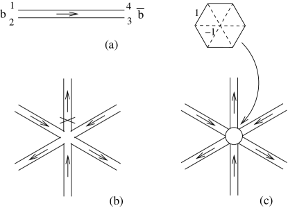
Figure 1: (a) Bare diffuson ${\cal D}^{(0)}_{\eta}(t)$. The arrow points in the direction of decreasing time. (b) Vertices arising from $S^{(\geq 4)}_{\rm E}[b,\bar{b}]$. Crossed diffuson denotes differentiation $\hat{\partial}b$ in the vertex (25). (c) Vertices arising from $S^{(\geq 4)}_{\rm kin}[b,\bar{b}]$. The vertex itself is characterized by a graph connecting different times $t_{i}$ at this vertex. The numbers on the links of the graph specify the coefficients $a^{(n)}_{ij}$ in (26).

The nonlinear vertices arising from $S^{(\geq 4)}_{\rm E}[b,\bar{b}]$ have the form

$$S^{(2n)}_{\rm E}[b,\bar{b}]=(-1)^{n+1}\pi\,c_{2n}\mathop{\rm Tr}\nolimits[(\hat{\partial}b)\bar{b}(b\bar{b})^{n-1}],$$ (25)

where we use the shorthand notation $(\hat{\partial}b)_{12}=(\partial_{1}+\partial_{2})b_{12}$, and the trace is understood as the convolution in time variables. The vertices from $S^{(\geq 4)}_{\rm kin}[b,\bar{b}]$ are of the form

$$S^{(2n)}_{\rm kin}[b,\bar{b}]=\alpha\int dt_{1}\dots dt_{2n}\,b_{12}\bar{b}_{23}\dots\bar{b}_{2n,1}\sum_{i<j}a_{ij}^{(n)}(t_{i}-t_{j})^{2},$$ (26)

where $a_{ij}^{(n)}$ are numerical coefficients expressed through the coefficients $c_{k}$ of the expansion (19):

$$a_{ij}^{(n)}=\frac{\pi}{2n}(-1)^{i-j+n}c_{j-i}c_{i-j+2n}.$$ (27)

Graphically, we order the diffusons at each vertex clockwise according to their appearance in the traces (25) and (26).

The average value of the physical observables is given by certain correlators of the original $Q$-field. When we compute them in terms of the $b$ and $\bar{b}$ fields, those observables generate “external vertices”. The vertices generated by $S^{(\geq 4)}_{\rm E}[b,\bar{b}]$ and $S^{(\geq 4)}_{\rm kin}[b,\bar{b}]$ will be further called “internal vertices”. Finally, vertices generated by the Jacobian $J_{f}[b,\bar{b}]$ (unless it equals one) we shall call “Jacobian vertices” (see Appendix B for the explicit form of the Jacobian vertices).

There are two obvious rules for constructing the diagrams. Firstly, the diffusons may be drawn on a planar figure without “twisting” (but intersections of different diffusons are allowed, see, e.g., Fig. 2c). Secondly, the diagram must not contain closed loops formed by internal lines. Such loops would immediately produce the factor $\theta(t_{1}-t_{2})\theta(t_{2}-t_{3})\dots\theta(t_{n}-t_{1})$ which always vanishes [note that $\theta(t_{1}-t_{1})=0$ due to the causality rule KamenevAndreev99 ; AltlandKamenev00 , and so loops of length one are not allowed either]. For example, the diagrams in Figs. 2ab identically vanish and should not be considered. An example of a non-vanishing two-loop diagram is shown in Fig. 2c.

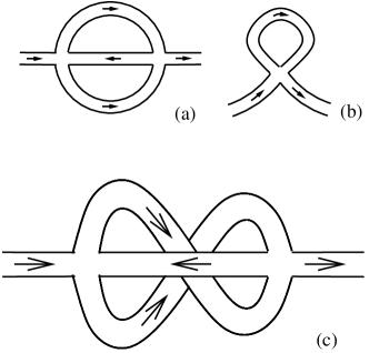
Figure 2: Examples of diagrams. Diagrams (a) and (b) trivially vanish. Panel (c) shows a non-vanishing two-loop diagram (this diagram is one of those considered in Refs. skvor, ; SBK04, ).

From the above constraints on the diagram we can prove that only even-loop diagrams contribute to the diffuson (15). More generally, the following theorem holds: Let $b^{(2n+1)}$ and $\bar{b}^{(2n+1)}$ denote the operators

$$b^{(2n+1)}_{tt^{\prime}} = \int b_{tt_{1}}\bar{b}_{t_{1}t_{2}}b_{t_{2}t_{3}}\dots b_{t_{2n}t^{\prime}}\,dt_{1}\,\dots\,dt_{2n},$$

$$\bar{b}^{(2n+1)}_{tt^{\prime}} = \int\bar{b}_{tt_{1}}b_{t_{1}t_{2}}\bar{b}_{t_{2}t_{3}}\dots\bar{b}_{t_{2n}t^{\prime}}\,dt_{1}\,\dots\,dt_{2n}.$$ (28)

Then any nonzero average $\langle b^{(n_{1})}\dots b^{(n_{k})}\,\bar{b}^{(\bar{n}_{1})}\dots\bar{b}^{(\bar{n}_{\bar{k}})}\rangle$ must contain equal number of $b$- and $\bar{b}$-operators and its diagrammatic expansion contains only diagrams with even number of loops.

Furthermore, from the same principle it is easy to prove that $\langle b^{(n)}_{t_{1}t_{2}}\bar{b}^{(\bar{n})}_{t_{3}t_{4}}\rangle=0$ if $t_{1}\leq t_{4}$ in all orders of the diagrammatic expansion. This proves the causality of the full diffuson (13): ${\cal D}_{\eta}(t\leq 0)=0$.

In the main body of the paper, we shall only use the rational parameterization:

$$f(W)=\frac{1+W/2}{1-W/2}.$$ (29)

The Jacobian for the rational parameterization is known Efetov1983 ; Efetov-book to be equal to 1. (In fact, such a parameterization is not unique. As shown in Appendix B, the class of parameterizations with unit Jacobian is given by a one-parameter family, with the rational parameterization being a particular representative.)

In the rational parameterization (29), the coefficients of the series (19) are given by $c_{k}=2^{1-k}$ ($k\geq 1$) and the coefficients $a_{ij}^{(n)}$ in the nonlinear vertices (26) have the form

$$a_{ij}^{(n)}=\frac{1}{n}\,(-1)^{i-j+n}2^{1-2n}\pi.$$ (30)

IV Diagrammatic series for the diffusion coefficient

In this section we apply the developed diagrammatic technique to calculating the full diffuson (13) and to further extracting the diffusion coefficient (16).

The observables in (13) have the form

$$Q^{(+)} = b^{(1)}-c_{3}b^{(3)}+c_{5}b^{(5)}-\dots,$$ (31)

$$Q^{(-)} = \bar{b}^{(1)}-c_{3}\bar{b}^{(3)}+c_{5}\bar{b}^{(5)}-\dots,$$ (32)

where $c_{3}$, $c_{5}$, …are the coefficients in the Taylor expansion of the parameterization (19), and the operators $b^{(n)}$ and $\bar{b}^{(n)}$ are defined in Eq. (28). Respectively, the average $\langle Q^{(+)}Q^{(-)}\rangle$ contains averages of different powers of $b$ and $\bar{b}$.

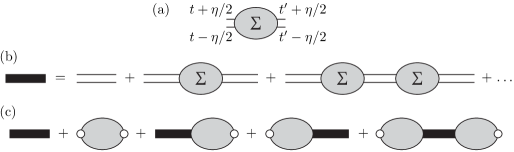
Figure 3: (a) Irreducible self-energy block $\Sigma_{\eta}(t-t^{\prime})$. (b) The diagrammatic expansion of the pro-diffuson $\langle b\bar{b}\rangle$ denoted by the solid propagator. (c) The diagrammatic expansion of the full diffuson $\langle Q^{(+)}Q^{(-)}\rangle$. The irreducible blocks differ from $\Sigma$ due to the presence of external vertices (shown by empty circles) containing higher powers of $b$ and $\bar{b}$.

Let us first discuss the simplest of those averages:

$$\langle b_{t+\eta/2,t-\eta/2}\bar{b}_{t^{\prime}-\eta^{\prime}/2,t^{\prime}+\eta^{\prime}/2}\rangle=\frac{2}{\pi}\delta(\eta-\eta^{\prime}){\cal D}^{*}_{\eta}(t-t^{\prime}).$$ (33)

Eq. (33) defines the “pro-diffuson” ${\cal D}^{*}_{\eta}(t)$ which should not be confused with the full diffuson given by Eq. (13). The pro-diffuson ${\cal D}^{*}_{\eta}(t)$ may be written in the perturbative series as shown in Fig. 3b. Defining the irreducible “self-energy” block $\Sigma_{\eta}(t)$ (shown pictorially in Fig. 3a) by the condition that it cannot be split in two pieces by cutting any one diffuson, we can resum the diagrammatic series for the pro-diffuson as

$$\bigl{[}{\cal D}^{*}_{\eta}(\omega)\bigr{]}^{-1}=\bigl{[}{\cal D}^{(0)}_{\eta}(\omega)\bigr{]}^{-1}-\Sigma_{\eta}(\omega).$$ (34)

Here we adopted the frequency representation, with

$${\cal D}^{(0)}_{\eta}(\omega)=\int_{-\infty}^{+\infty}e^{i\omega t}{\cal D}^{(0)}_{\eta}(\omega)\,dt=\frac{1}{-i\omega+\alpha\eta^{2}}.$$ (35)

The role of the self-energy $\Sigma_{\eta}(\omega)$ is shifting the pole of the pro-diffuson ${\cal D}^{*}_{\eta}(\omega)$.

One can see that the bare diffuson (35) in the frequency representation looks exactly as the diffuson propagator $1/(-i\omega+Dq^{2})$ for a particle in a disordered medium. However, the analogy between these problems does not extend beyond the formal coincidence of the bare propagators. Indeed, for a particle in a random potential, the frequency $\omega$ and momentum $q$ are “decoupled” from each other: each diffuson in a diagram has the same frequency, while the choice of their momenta $q_{i}$ is dictated by the momentum conservation law in the vertices. Contrary, for the dynamic problem, the times $\eta_{i}$ and $t_{j}$ of the internal diffusons ${\cal D}^{(0)}_{\eta_{i}}(t_{i})$ which constitute the self-energy block $\Sigma_{\eta}(t)$ are linearly related to each other (see Section VI for their explicit form). Therefore, in the frequency representation, the internal diffusons in $\Sigma_{\eta}(\omega)$ will enter with different frequencies $\omega_{i}$ coupled to the time arguments $\eta_{j}$. Thus, the frequency representation (35) is not a way to calculate $\Sigma_{\eta}(t)$, but is a convenient tool for summing the geometric series (34).

Note that the full diffuson ${\cal D}_{\eta}(t)$ differs from the pro-diffuson ${\cal D}^{*}_{\eta}(t)$ by higher-power averages $\langle b^{(n)}\cdot\bar{b}^{(\bar{n})}\rangle$ (see Fig. 3c). We observe that all irreducible parts [both $\Sigma_{\eta}(t)$ and the irreducible blocks in Fig. 3c] remain exponentially decaying with time even at $\eta=0$ (in the frequency representation, they are non-singular functions of $\eta$ and $\omega$ at $\eta\to 0$ and $\omega\to 0$) convergence . Therefore we may sum all the diagrams to the form

$${\cal D}_{\eta}(\omega)=\frac{Z(\eta,\omega)}{-i\omega+\alpha\eta^{2}-\Sigma_{\eta}(\omega)},$$ (36)

where $Z(\eta,\omega)$ is a regular function at $\eta\to 0$ and $\omega\to 0$. As we shall see from the further explicit calculations, $\Sigma_{\eta}(\omega)\to 0$ as $\eta\to 0$. Furthermore, the full diffuson ${\cal D}_{\eta}(\omega)$ remains unrenormalized at $\eta=0$ (see Appendix A for a proof). Therefore, $Z(\eta=0,\omega)=1$.

Thus the correction to the diffusion coefficient is determined by the leading term in the expansion of $\Sigma_{\eta}(\omega)$ in $\eta$ and $\omega$:

$$D(\alpha)=\alpha-\lim_{\eta\to 0}\frac{\Sigma_{\eta}(\omega=0)}{\eta^{2}}=\alpha-\lim_{\eta\to 0}\frac{1}{\eta^{2}}\int_{0}^{\infty}\Sigma_{\eta}(t)\,dt,$$ (37)

where the lower limit of $t$-integration follows from the causality of $\Sigma_{\eta}(t)$ which can be proved analogously to the causality of the diffuson ${\cal D}_{\eta}(t)$.

The diagrams representing the irreducible block $\Sigma_{\eta}(t)$ may be classified in the number of loops $L$. From simple power counting (as shown in Ref. skvor, ) the $L$-loop diagrams give a contribution to $D(\alpha)$ proportional to $\alpha^{1-L/3}$, cf. Eq. (6). Therefore, the diagrammatic expansion is a series in the number of loops, and (since the number of loops $L$ must be even) the expansion small parameter is $\alpha^{-2/3}$, up to some unknown number. A more accurate analysis of Sec. VI shows that the actual small parameter is $\pi^{-2}\alpha^{-2/3}$.

In the following section we shall see that certain different diagrams with the same number of loops $L$ may partially cancel each other.

V Canceling vertices of order higher than four

In this section we show that, in the rational parameterization (29), in diagrams containing only internal vertices (e.g., in $\Sigma_{\eta}(t)$), all vertices of order higher than four are cancelled in all orders of the diagram series.

The outline of the calculation is as follows. The vertices with derivatives originating from $S_{\rm E}^{(\geq 4)}$ (Fig. 1b) generate terms $\partial_{t}{\cal D}^{(0)}_{\eta}(t)$. We transform those terms according to the equation of motion for the diffuson:

$$\partial_{t}{\cal D}^{(0)}_{\eta}(t)=\delta(t)-\alpha\eta^{2}{\cal D}^{(0)}_{\eta}(t).$$ (38)

The resulting expressions have the form of $(t_{i}-t_{j})^{2}$ vertices in Fig. 1c and may then be combined with the vertices originally generated by $S^{(\geq 4)}_{\rm kin}[b,\bar{b}]$.

When performed in the rational parameterization (29), this procedure leads to the cancellation of all vertices of order higher than four in all orders of the perturbation series. The calculation is somewhat technical with the combinatoric counting of diagrams and coefficients. This calculation is reported in detail in Appendix C.

Of course, at the end of the above simplification procedure, the fourth-order vertices get modified from their original form. The final form of the fourth-order vertex is

$$S^{*}_{4}[b,\bar{b}]=-\frac{\pi\alpha}{8}\int dt_{1}\,dt_{2}\,dt_{3}\,dt_{4}\,(t_{1}-t_{2})(t_{3}-t_{4})\,b_{12}\bar{b}_{23}b_{34}\bar{b}_{41}.$$ (39)

The resulting theory in terms of $b$-fields (which we will further call “$b$-theory”) has the action

$$S_{\rm eff}[b,\bar{b}]=S^{(2)}[b,\bar{b}]+S^{*}_{4}[b,\bar{b}],$$ (40)

where $S^{(2)}[b,\bar{b}]$ is given by (22).

We need to make two comments on the above derivation.

First, up to now the correspondence is established only between diagrams containing internal vertices. The correspondence between physical observables (i.e., external vertices) will be discussed in Section IX. In the further discussion, we employ the $b$-theory for calculating $\Sigma_{\eta}(t)$ which contains only internal vertices.

Second, when constructing the diagrams for $\Sigma_{\eta}(t)$ in the $b$-theory, one of the $(t_{2i-1}-t_{2i})$ factors in $S^{*}_{4}[b,\bar{b}]$ always coincides with the external time difference $\eta$. The integrals over times $t_{i}$ converge convergence and therefore

$$\Sigma_{\eta=0}(t)=0.$$ (41)

Obviously $\Sigma_{\eta}(t)$ is an even and regular function of $\eta$. Thus the Taylor expansion of $\Sigma_{\eta}(t)$ in small $\eta$ starts with $\eta^{2}$. The leading term in this expansion determines the correction to the diffusion coefficient, according to (37). We shall perform an explicit calculation in the next section.

VI Diagrammatic expansion for $D(\alpha)$

In this section we classify the diagrams for $\Sigma_{\eta}(t)$ in the $b$-theory (40) and write down explicit integral expressions for the correction to the diffusion coefficient (37).

Consider any diagram (in the $b$-theory) with $L$ loops contributing to $\Sigma_{\eta}(t)$. As mentioned previously, such a diagram must contain no closed threads, which greatly restricts the number of allowed diagrams (in particular, the number of loops $L$ must be even). Since all the vertices in the $b$-theory have valency four, the number of diffusons in the diagram is $2L-1$. We enumerate those diffusons in two different sequences which we shall call the “left-hand” and “right-hand” numberings. Start at the “entry point” (external diffuson leading into the diagram) and go along the diffusons in two different ways: using the right-hand rule (following the right edges of the diffusons, i.e., turning right at every vertex) and using the left-hand rule (following the left edges of the diffusons and turning left at every vertex). The relative re-numbering of the diffusons in the two sequences defines a permutation $\sigma$ of $(2L-1)$ elements. In other words, let us number the diffusons following the right-hand route. Then reading off the diffuson numbers along the left-hand route produces the sequence of numbers [$\sigma(1)$, $\sigma(2)$,…, $\sigma(2L-1)$]. We shall further label the diagrams by such sequences (see Table 1). An example of the 4-loop diagram corresponding to the permutation $\sigma=[3764215]$ (numbered 2 in the Table 1) is shown in Fig. 4.

No.	$\sigma$	comments
1	[3214765]	reducible
2	[3764215]
3	[3752164]
4	[3621754]
5	[3654721]
6	[4276315]	= No. 3 (T)
7	[4731652]
8	[4317625]	= No. 4 (LR/T)
9	[4726531]
10	[5274163]
11	[5417362]	= No. 3 (LR)
12	[5372641]
13	[6327514]	= No. 7 (T)
14	[6514732]	= No. 2 (LR)
15	[6251743]	= No. 3 (LR+T)
16	[6437251]	= No. 9 (LR+T)
17	[7614325]	= No. 5 (LR/T)
18	[7532614]	= No. 9 (T)
19	[7426153]	= No. 12 (LR/T)
20	[7361542]	= No. 9 (LR)
21	[7254361]

Table 1: The list of all four-loop diagrams for the self-energy part $\Sigma$. Each diagram is characterized by a permutation $\sigma$, see text. The diagram No. 1 is reducible: it can be written as $\Sigma_{2}{\cal D}^{(0)}\Sigma_{2}$, where $\Sigma_{2}$ is the two-loop contribution. The other diagrams are irreducible. The diagrams related by the “left-right” (LR) or time-reversal (T) symmetries give the same contribution. LR+T means that two diagrams are related by the combined action of the two symmetries. LR/T indicate that two symmetries applied to a permutation give the same result. Graphical representation of the diagram No. 2 is given in Fig. 4.

Figure 4: An example of the 4-loop diagram for the self-energy $\Sigma$. This diagram corresponds to the permutation $\sigma=[3764215]$ listed as No. 2 in the Table 1.

Note that not every permutation of $2L-1$ elements defines a diagram. We do not discuss here the combinatoric problem of enumerating all diagrams in all orders. For our modest purpose of calculating the four-loop correction to the diffusion coefficient, the enumeration of the diagrams may be easily done “by hand”. Recall that for $L=2$ there is only one allowed diagram (shown in Fig. 2) corresponding to the permutation [3,2,1]. For $L=4$, the number of allowed diagrams (and the corresponding permutations) is 21, see Table 1. Note that one of those diagrams (No. 1 in Table 1) is reducible: it consists of two independent two-loop blocks.

Given a diagram characterized by a certain permutation $\sigma$, let $\eta_{i}$ and $t_{i}$ denote the parameters of the diffusons ${\cal D}^{(0)}_{\eta_{i}}(t_{i})$ involved in the diagram, with the diffusons enumerated along the right-hand route. For calculating the diagram, it is convenient to take $t_{1},\dots,t_{2L-1}$ as independent integration variables. The parameters $\eta_{i}$ may be expressed via $t_{i}$ as

$$\eta_{i}=\eta+\sum_{j<i}t_{j}-\sum_{\sigma(j)<\sigma(i)}\!\!\!\!t_{j}=\eta+\sum_{j}\gamma^{(\sigma)}_{ij}t_{j}.$$ (42)

Here the first (second) sum contains all times $t_{j}$ encountered before $t_{i}$ along the right-hand (left-hand, respectively) route. The last equality is the definition of the coefficients $\gamma^{(\sigma)}_{ij}$. The matrix $\gamma^{(\sigma)}_{ij}$ contains only entries $0$, $1$, and $-1$, and is antisymmetric: $\gamma^{(\sigma)}_{ij}=-\gamma^{(\sigma)}_{ji}$. Moreover, the elements $\gamma^{(\sigma)}_{ij}$ with $i>j$ are non-negative (either 0 or 1), and those with $i<j$ are non-positive (either 0 or $-1$).

Finally, calculating the self-energy block $\Sigma_{\eta}(t)$ in the $b$-theory (40) and employing Eq. (37), we may write down the contribution of any given irreducible diagram (corresponding to a given permutation $\sigma$) to the diffusion coefficient $D(\alpha)$:

$$\delta^{(\sigma)}D(\alpha)=-\frac{K^{(\sigma)}}{\pi^{L}}\alpha^{1-L/3},$$ (43)

where

$$K^{(\sigma)}=\int_{0}^{\infty}\!\!\!\!\dots\int_{0}^{\infty}\left(\prod_{i=1}^{2L-1}dT_{i}\right)P^{(\sigma)}(T_{1},\dots,T_{2L-1})e^{-S_{3}^{(\sigma)}(T_{1},\dots,T_{2L-1})}.$$ (44)

Here $P^{(\sigma)}(T_{1},\dots,T_{2L-1})$ and $S_{3}^{(\sigma)}(T_{1},\dots,T_{2L-1})$ are homogeneous polynomials of degrees $2L-2$ and three, respectively. They are defined as

$$P^{(\sigma)}(T_{1},\dots,T_{2L-1}) =\left(\prod_{i=1}^{2L-1}{\tilde{\eta}}_{i}\right)\sum_{i=1}^{2L-1}\frac{1}{{\tilde{\eta}}_{i}},$$ (45a)

$$S_{3}^{(\sigma)}(T_{1},\dots,T_{2L-1}) =\sum_{i=1}^{2L-1}{\tilde{\eta}}_{i}^{2}T_{i},$$ (45b)

$${\tilde{\eta}}_{i} =\sum_{j}\gamma^{(\sigma)}_{ij}T_{j},$$ (45c)

where the coefficients $\gamma^{(\sigma)}_{ij}$ are constructed from the permutation $\sigma$ according to Eq. (42).

No.	$M^{(\sigma)}$	$K^{(\sigma)}$	st. dev.
2	2	0.066945	0.000015
3	4	$-0.123205$	0.000012
4	2	0.082358	0.000018
5	2	0.008234	0.000005
7	2	0.006030	0.000007
9	4	$-0.006567$	0.000005
10	1	0.206687	0.000013
12	2	$-0.001646$	0.000006
21	1	$-0.011374$	0.000003

Table 2: Results of numerical evaluation of the diagrams from Table 1. $M^{(\sigma)}$ denote the multiplicities of the diagrams. $K^{(\sigma)}$ is given by Eq. (44). The last column is the standard deviation of $K^{(\sigma)}$.

VII Numerical calculation of the 4-loop diagrams

The list of allowed four-loop diagrams (permutations) is given in Table 1. The first diagram in the list is not irreducible: it consists of two blocks of two loops each and should not be included in the irreducible part $\Sigma_{\eta}(t)$. Out of the remaining 20 diagrams, some are related by symmetries and produce the same contributions (44). Namely, there are two possible symmetries: the “left-right” (LR) reflection of the diffusons (corresponding to the transformation $\sigma\mapsto\sigma^{-1}$) and the time-reversal (T) symmetry (corresponding to replacing $\sigma(i)\mapsto 2L-\sigma(2L-i)$). The diagrams related by the symmetries are identified in the above table. It remains to calculate the nine different diagrams and add them with the corresponding multiplicities $M^{(\sigma)}$, see Table 2.

The antisymmetric matrices $\gamma^{(\sigma)}$ defined for nine permutations $\sigma$ from Table 2 are listed below, with the elements $+$ ($-$) standing for 1 ($-1$) for brevity:

$$\gamma^{(2)}=\left[\begin{array}[]{ccccccc}0&-&-&-&0&-&-\\ +&0&-&-&0&-&-\\ +&+&0&0&0&0&0\\ +&+&0&0&0&-&-\\ 0&0&0&0&0&-&-\\ +&+&0&+&+&0&-\\ +&+&0&+&+&+&0\end{array}\right];\quad\gamma^{(3)}=\left[\begin{array}[]{ccccccc}0&-&-&0&-&0&-\\ +&0&-&0&-&0&-\\ +&+&0&0&0&0&0\\ 0&0&0&0&-&-&-\\ +&+&0&+&0&0&-\\ 0&0&0&+&0&0&-\\ +&+&0&+&+&+&0\end{array}\right];\quad\gamma^{(4)}=\left[\begin{array}[]{ccccccc}0&-&-&0&0&-&0\\ +&0&-&0&0&-&0\\ +&+&0&0&0&0&0\\ 0&0&0&0&-&-&-\\ 0&0&0&+&0&-&-\\ +&+&0&+&+&0&0\\ 0&0&0&+&+&0&0\end{array}\right];$$ (67)

$$\gamma^{(5)}=\left[\begin{array}[]{ccccccc}0&-&-&-&-&-&-\\ +&0&-&-&-&-&-\\ +&+&0&0&0&0&0\\ +&+&0&0&-&-&0\\ +&+&0&+&0&-&0\\ +&+&0&+&+&0&0\\ +&+&0&0&0&0&0\end{array}\right];\quad\gamma^{(7)}=\left[\begin{array}[]{ccccccc}0&0&-&-&0&0&-\\ 0&0&-&-&-&-&-\\ +&+&0&-&0&0&-\\ +&+&+&0&0&0&0\\ 0&+&0&0&0&-&-\\ 0&+&0&0&+&0&-\\ +&+&+&0&+&+&0\end{array}\right];\quad\gamma^{(9)}=\left[\begin{array}[]{ccccccc}0&-&-&-&-&-&-\\ +&0&0&-&0&0&-\\ +&0&0&-&-&-&-\\ +&+&+&0&0&0&0\\ +&0&+&0&0&-&-\\ +&0&+&0&+&0&-\\ +&+&+&0&+&+&0\end{array}\right];$$ (89)

$$\gamma^{(10)}=\left[\begin{array}[]{ccccccc}0&-&0&-&-&0&-\\ +&0&0&0&-&0&0\\ 0&0&0&-&-&-&-\\ +&0&+&0&-&0&-\\ +&+&+&+&0&0&0\\ 0&0&+&0&0&0&-\\ +&0&+&+&0&+&0\end{array}\right];\quad\gamma^{(12)}=\left[\begin{array}[]{ccccccc}0&-&-&-&-&-&-\\ +&0&-&0&-&0&-\\ +&+&0&0&-&0&0\\ +&0&0&0&-&-&-\\ +&+&+&+&0&0&0\\ +&0&0&+&0&0&-\\ +&+&0&+&0&+&0\end{array}\right];\quad\gamma^{(21)}=\left[\begin{array}[]{ccccccc}0&-&-&-&-&-&-\\ +&0&0&0&0&0&-\\ +&0&0&-&-&0&-\\ +&0&+&0&-&0&-\\ +&0&+&+&0&0&-\\ +&0&0&0&0&0&-\\ +&+&+&+&+&+&0\end{array}\right].$$ (111)

Here, the matrix $\gamma^{(m)}$ denotes the matrix $\gamma^{(\sigma)}$ for the permutation No. $m$ from the Table 2.

The results of Monte Carlo numeric evaluation of the seven-fold integrals $K^{(\sigma)}$ given by Eq. (44) are summarized in Table 2. Performing summation with the multiplicities $M^{(\sigma)}$ we get finally the estimate for the coefficient $d_{4}$ in the Taylor expansion (6):

$$d_{4}=-(7\pm 7)\times 10^{-5}.$$ (112)

The numerical uncertainty indicated in Eq. (112) corresponds to one standard deviation. Thus, we cannot distinguish $d_{4}$ from zero and can estimate the upper bound for its absolute value as $|d_{4}|<3\times 10^{-4}$.

VIII Arbitrary dependence of $\varphi(t)$

In this section we discuss to what extent the results obtained above can be generalized to an arbitrary time dependence of the control parameter $\varphi(t)$.

We start by summarizing the modifications of the theory introduced by an arbitrary $\varphi(t)$. For a generic $\varphi(t)$, the diffuson becomes a function of three times [cf. Eq. (13)]:

$$\langle Q^{(+)}_{t+\eta/2,t-\eta/2}Q^{(-)}_{t^{\prime}-\eta^{\prime}/2,t^{\prime}+\eta^{\prime}/2}\rangle=\frac{2\Delta}{\pi}\delta(\eta-\eta^{\prime}){\cal D}_{\eta}(t,t^{\prime}).$$ (113)

To study the action (8) one can develop the standard perturbation theory described in Section III. In terms of the $b$-fields, the action will have the form (21) with the quadratic part ($\varphi_{i}\equiv\varphi(t_{i})$)

$$S^{(2)}[b,\bar{b}]=\frac{\pi}{2\Delta}\int\!\!\int dt_{1}\,dt_{2}\,\bar{b}_{12}\Big{[}(\partial_{1}+\partial_{2})+\Gamma(\varphi_{1}-\varphi_{2})^{2}\Big{]}b_{21}$$ (114)

and infinite number of nonlinear terms $S^{\geq 4}[b,\bar{b}]$. In Eq. (114) we introduced $\Gamma=\pi\Delta C(0)$. The bare diffuson defined as the propagator of $S^{(2)}[b,\bar{b}]$ is given by AAK1982 ; VavilovAleiner1999 ; SBK04

$${\cal D}^{(0)}_{\eta}(t,t^{\prime})=\theta(t-t^{\prime})\exp\left\{-\Gamma\int_{t^{\prime}}^{t}[\varphi(\tau+\eta/2)-\varphi(\tau-\eta/2)]^{2}d\tau\right\}.$$ (115)

It is remarkable that with such a modification of the theory one can still prove the cancellation of all internal vertices of the order higher than 4 in the rational parameterization. Indeed, the proof presented in Section V was based on the equation of motion (38) for the diffuson, which is now replaced by an analogous equation

$$\partial_{t}{\cal D}^{(0)}_{\eta}(t,t^{\prime})=\delta(t-t^{\prime})-\Gamma[\varphi(t+\eta/2)-\varphi(t-\eta/2)]^{2}{\cal D}^{(0)}_{\eta}(t,t^{\prime}),$$ (116)

and the combinatorial counting of coefficients which is insensitive to time dependence of $\varphi(t)$.

The resulting $b$-theory has the action

$$S=S^{(2)}[b,\bar{b}]-\frac{\pi\Gamma}{8\Delta}\int dt_{1}dt_{2}dt_{3}dt_{4}\,(\varphi_{1}-\varphi_{2})(\varphi_{3}-\varphi_{4})\,b_{12}\bar{b}_{23}b_{34}\bar{b}_{41},$$ (117)

which is a generalization of Eq. (40) for an arbitrary dependence of the control parameter $\varphi(t)$. Thus, the diagrams for the pro-diffuson $\langle b\bar{b}\rangle$:

$$\langle b_{t+\eta/2,t-\eta/2}\bar{b}_{t^{\prime}-\eta^{\prime}/2,t^{\prime}+\eta^{\prime}/2}\rangle=\frac{2\Delta}{\pi}\delta(\eta-\eta^{\prime}){\cal D}^{*}_{\eta}(t,t^{\prime})$$ (118)

with an arbitrary $\varphi(t)$ are exactly the same as the diagrams in the linear case $\varphi(t)=vt$ considered in the previous Sections (but with the new diffusons (115)).

The energy absorption rate is expressed through the full diffuson ${\cal D}_{\eta}(t,t^{\prime})$ defined in terms of the field $Q$ by Eq. (113). It differs from the pro-diffuson ${\cal D}^{*}_{\eta}(t,t^{\prime})$ in the $b$-theory since $Q$ is a nonlinear function of $b$ and $\bar{b}$. In studying the linear perturbation this difference was irrelevant for the calculation of the diffusion coefficient (see Section VI). For a generic perturbation $\varphi(t)$, the difference between the full diffuson ${\cal D}_{\eta}(t,t^{\prime})$ and the pro-diffuson ${\cal D}^{*}_{\eta}(t,t^{\prime})$ becomes important. In particular, the two-loop analysis of the quantum interference correction under the action of a harmonic perturbation SBK04 has shown that the average $\langle b\bar{b}b\cdot\bar{b}\rangle$ (the diagram (c) in Ref. SBK04, ) has a contribution comparable to that of the average $\langle b\cdot\bar{b}\rangle$, both being negative and growing with time $\propto t$.

IX Relation to the Dyson-Maleev transformation

In this section we elucidate the meaning of the effective $b$-theory (40) and discuss its relation to the Dyson-Maleev transformation widely used in dealing with quantum spin ferromagnets.

The action (40) has been obtained in the previous sections from an analysis of mutual cancellations of higher-order vertices in the perturbation theory for the rational parameterization. However, it turns out that the same action may be obtained directly from the initial $\sigma$-model action (9) if one adopts the following parameterization of the $Q$-matrix in terms of the fields $b$ and $\bar{b}$:

$$Q=\begin{pmatrix}1-b\bar{b}/2&&b-b\bar{b}b/4\\ \bar{b}&&-1+\bar{b}b/2\end{pmatrix}.$$ (119)

Indeed, this parameterization respects the nonlinear constraint $Q^{2}=1$, and the trivial algebra of substituting (119) into the initial $\sigma$-model action (9) immediately leads to the effective action (40) of the $b$-theory. With the explicit parameterization (119), external vertices (matrix elements of the $Q$-matrix) also become finite polynomials in $b$ and $\bar{b}$. We have checked that the two approaches (direct use of the parameterization (119) and the vertex cancellation by the technique developed in Appendix C) produce the same effective external vertices.

Thus we come to an important conclusion about the $\sigma$-model (9): The rational parameterization (29) (which contains an infinite series of higher-order interaction vertices) after mutual cancellation of higher-order vertices in the diagrammatic expansion is perturbatively equivalent to the parameterization (119).

In the rational parameterization [more generally, in any parameterization of the form (18)–(20)], the matrices $b$ and $\bar{b}$ are Hermitian conjugate of each other: $\bar{b}=b^{\dagger}$. The same remains therefore true for the $b$-theory (40) obtained from the rational parameterization. On the other hand, the parameterization (119) with $\bar{b}=b^{\dagger}$ violates the hermiticity of the $Q$ matrix. Nevertheless, our derivation indicates that this violation is inessential at the perturbative level and can be taken into account by a proper deformation of the integration contour over the elements of the $Q$ matrix.

The parameterization (119) is closely related to the famous Dyson-Maleev Dyson56 ; Maleev57 parameterization for quantum spins. In that representation, the spin-$S$ operators are expressed by the boson creation and annihilation operators $\hat{a}^{\dagger}$ and $\hat{a}$ as

$$\hat{S}^{+}=(2S-\hat{a}^{\dagger}\hat{a})\hat{a},\qquad\hat{S}^{-}=\hat{a}^{\dagger},\qquad\hat{S}^{z}=S-\hat{a}^{\dagger}\hat{a}.$$ (120)

The Dyson-Maleev transformation conserves the spin commutation relations but violates the property $(\hat{S}^{-})^{\dagger}=\hat{S}^{+}$ rendering the spin Hamiltonian manifestly non-Hermitian. This is the expense one has to pay for making the spin Hamiltonian a finite-order polynomial in boson operators [as opposed to an infinite series in the Holstein-Primakoff parameterization HolstPrim40 ; note that the Holstein-Primakoff parameterization is analogous to the square-root-even parameterization (151)]. The Dyson-Maleev transformation has proven to be the most convenient tool for studying spin wave interaction Canali92 ; Hamer92-93 : it reproduces all the perturbative results obtained with the Holstein-Primakoff parameterization in a much faster and compact way.

A classical analogue of the Dyson-Maleev transformation was recently used by Kolokolov Kolokolov2000 in studying two-dimensional classical ferromagnets. To the best of our knowledge, there exists just one article by Gruzberg, Read and Sachdev Gruzberg1997 where the Dyson-Maleev parameterization was applied for the perturbative treatment of a $\sigma$-model (in the replica form).

In the Dyson-Maleev representation, the Hilbert space of free bosons should be truncated in order for the operator $\hat{S}^{z}$ to have a bounded spectrum. In Ref. Kolokolov2000, , this truncation corresponds to integrating over a bounded region in bosonic variables. We expect that a similar constraint on the matrices $b$ and $\bar{b}$ may be required in order to achieve a nonperturbative equivalence between the initial $\sigma$-model in the $Q$-representation and the $b$-theory. This question is of importance for studying non-perturbative effects in $\sigma$-models, but goes beyond the scope of the present paper.

X Discussion

This work has appeared as a result of our attempt to prove the conjecture formulated in Ref. skvor, that the Kubo formula for the energy absorption rate of a linearly driven unitary random Hamiltonian gives an exact result in the whole range of driving velocities. In the notation of the present paper, this conjecture implies that the relation $D(\alpha)=\alpha$ is exact.

Being unable to verify the conjecture nonperturbatively, we calculate the four-loop correction to the Kubo formula $D(\alpha)=\alpha$ in the limit of large velocities of the driving field, $\alpha\gg 1$. In the process of our derivation, we have refined the $\sigma$-model approach of Ref. skvor, : our improved method does not involve the fermionic distribution function and expresses the energy diffusion coefficient (16) in terms of the full diffuson (13) of the field theory (9).

We have further proven that the resulting $\sigma$-model is perturbatively equivalent to the specific matrix $\phi^{4}$-theory (40). The lack of higher nonlinearities makes it possible to classify all four-loop diagrams and write down analytic expressions for them without resorting to computer symbolic computations. The final evaluation of emerging 7-dimensional integrals (44) cannot be done analytically, and we calculate them numerically. We find that the coefficient $d_{4}$ in the expansion (6) is indistinguishable from zero within the precision of our calculation, with its absolute value bounded by $|d_{4}|<3\times 10^{-4}$.

We believe that this conclusion acts in favor of the conjecture $D(\alpha)=\alpha$.

This result may appear less surprising if we recall that the static (time-independent) unitary random-matrix ensemble is also known to possess some peculiar properties. In particular, its spectral statistics can be mapped onto the problem of one-dimensional noninteracting fermions; for a certain class of integrals over the unitary group the saddle-point approximation is exact (the Duistermaat-Heckman theorem Duistermaat-Heckman , see Ref. Zirnbauer99, for a discussion). However, in the time-dependent problem considered in the present work, we are not able to perform mapping onto free fermions, and the Duistermaat-Heckman theorem does not help to evaluate the functional integral of the Keldysh $\sigma$-model. The $\sigma$-model is nontrivial, and its diffuson ${\cal D}_{\eta}(t)$ is a complicated function of $\eta$ and $t$ at arbitrary value of the coupling $\alpha$. The diffuson ${\cal D}_{\eta}(t)$ is renormalized from the simple diffusive form (24), and our result indicates that only its long-time asymptotics [which determines the energy diffusion coefficient (16)] is free from perturbative corrections up to the order $\alpha^{-4/3}$.

The verification of the original nonperturbative conjecture $D(\alpha)=\alpha$ remains an open question.

As a byproduct of our analysis, we have rederived the $Q$-matrix parameterization (119) which is analogous to the Dyson–Maleev parameterization for spin operators Gruzberg1997 . The parameterization (119) is not specific to the Keldysh formalism, and can be applied to a wide class of unitary $\sigma$-models (e.g., to that describing diffusion of a particle in random media, both in the supersymmetric or replica Gruzberg1997 approaches), leading to a considerable simplification of the perturbative expansion. We could not extend this parameterization to the orthogonal and symplectic $\sigma$-models, since those involve additional linear constraints on the $Q$-matrix, apparently incompatible with our parameterization.

Appendix A Ward identity and energy absorption rate

In this Appendix we show that in the many-particle formulation the energy absorption rate under the action of an arbitrary perturbation $\varphi(t)$ is expressed through the generalized diffuson (113). In particular, for the linear perturbation $\varphi(t)=vt$, the diffusion coefficient in the energy space may be extracted from the decay rate of the diffuson (13). As a byproduct of our discussion, we also prove that, at $\eta=0$, the diffuson reduces to the step function:

$${\cal D}_{\eta=0}(t)=\theta(t)\,.$$ (121)

A.1 Two approaches to energy diffusion

The diffusion coefficient in the energy space may be defined in two different ways.

In the original sigma-model derivation skvor , the states of the time-dependent Hamiltonian $H(t)$ were occupied by noninteracting fermions. In such a multi-particle formulation, the step-like structure of the fermionic distribution function $f(E)$,

$$\lim_{E\to-\infty}f(E)=1,\qquad\lim_{E\to\infty}f(E)=0,$$ (122)

generates a spectral flow of fermions from low to high energies leading to the increase of the total energy of the system with time. At large time and energy scales, this many-particle process may be described by a diffusion equation on the distribution function $f(E)$. The corresponding diffusion coefficient expressed as $D\Delta^{3}$ (where $\Delta$ is the average interlevel spacing and $D$ is dimensionless) translates into the energy pumping rate $W=D\Delta^{2}$ (the density of states is $\Delta^{-1}$).

On the other hand, the same diffusion process may be observed in a single-particle problem. In the single-particle quantum mechanics (1), the energy of the system $E(t)$ defined with the instantaneous Hamiltonian

$$E(t)=\langle\Psi(t)|H(t)|\Psi(t)\rangle$$ (123)

diffuses with time as described by (4). One can expect that in the process of time evolution of $H(t)$, the relative phases of the wave function components corresponding to widely separated energies become uncorrelated, and therefore the multi-particle diffusion evolution of $f(E)$ and the single-particle diffusion process give equivalent definitions of the diffusion coefficient $D$. The above reasoning is justified for a non-periodic evolution of $H(t)$ (for example, for the linear evolution of the parameter $\varphi(t)=vt$); for a periodic perturbation studied in Ref. BSK03, , the phase correlations become important which leads to dynamic localization. Nevertheless, we show below that the energy pumping rate $W$ in the multi-particle problem may be expressed in terms of the single-particle diffuson for a rather general time dependence $\varphi(t)$.

A.2 Ward identity

A helpful tool for our further derivation are the Ward identities generated by rotations of the integration variables $Q$ in the functional integral of the sigma-model.

Consider the functional

$$\Pi[V]=\int V^{-1}QV\,e^{-S[V^{-1}QV]}[DQ],$$ (124)

where $V$ is an arbitrary matrix in the time and Keldysh spaces (not necessarily unitary), and the action is given by Eq. (8). The integration is performed over the matrices $Q$ of the form (11), (12). If the rotation by the matrix $V$ is local (with $V_{tt^{\prime}}\to\delta_{tt^{\prime}}$ at $|t|,|t^{\prime}|\to\infty$), it may be compensated by changing the integration variable $Q\mapsto V^{-1}QV$ in Eq. (124) producing no anomalous contribution, and therefore $\Pi[V]$ is independent of such rotations $V$.

The multi-particle approach described in the previous subsection may also be introduced with the same rotated path integral (124), but with the anomalous rotation matrix $V$ (involving the distribution function $f(E)$) skvor . This anomalous rotation will be discussed in detail below in the subsequent subsection, and in this subsection we derive the Ward identity generated by infinitesimal non-anomalous rotations $V$.

Expanding $V=1+A+\dots$ and taking the variation of $\Pi[V]$ with respect to the infinitesimal generator $A$ we get

$$\delta\Pi=[\langle Q\rangle,A]+\frac{\pi i}{\Delta}\langle Q\mathop{\rm Tr}\nolimits([Q,\hat{E}]A)\rangle+\pi^{2}C(0)\langle Q\mathop{\rm Tr}\nolimits([\hat{\varphi},Q\hat{\varphi}Q]A)\rangle=0\,.$$ (125)

In deriving the second term with $[Q,\hat{E}]$ we performed a cyclic permutation under the trace, which is equivalent to integration by parts and omitting the resulting boundary terms. This procedure is justified for local $A_{tt^{\prime}}$.

Various components of Eq. (125) associated with different elements of the matrix $A$ give the set of Ward identities related to the $V$-invariance of $\Pi[V]$. Of particular importance is its off-diagonal (Keldysh) component $\Pi^{(+)}$ generated by the Keldysh element $A^{(+)}$:

$$\delta_{t_{1}t_{4}}\delta_{t_{2}t_{3}}+\delta_{t_{1}-t_{2},t_{4}-t_{3}}(\partial_{3}+\partial_{4})\,{\cal D}_{t_{1}-t_{2}}\!\left(\frac{t_{1}+t_{2}}{2},\frac{t_{3}+t_{4}}{2}\right)+\frac{\pi^{2}}{2}C(0)(\varphi_{3}-\varphi_{4})\int dt_{5}\,\varphi_{5}\,\langle Q^{(+)}_{12}(Q_{35}Q_{54})^{(-)}\rangle=0,$$ (126)

where the diffuson with three times ${\cal D}_{\eta}(t,t^{\prime})$ is defined in Eq. (113) for an arbitrary time dependence $\varphi(t)$, and we have used that, due to causality, $\langle Q_{tt^{\prime}}\rangle=\Lambda=\sigma_{3}\delta_{tt^{\prime}}$.

A.3 Causality of the diffuson

The diffuson ${\cal D}_{\eta}(t,t^{\prime})$ may be calculated by summing the diagrammatic series as described in Section III. Every line in the diagram is the bare retarded diffuson (115), and therefore the full diffuson ${\cal D}_{\eta}(t,t^{\prime})$ also equals zero when $t<t^{\prime}$.

Furthermore, using the Ward identity (126) at $\eta=0$, we immediately find that the diffuson ${\cal D}_{\eta}(t,t^{\prime})$ reduces to the step function of $t-t^{\prime}$. Indeed, setting $t_{3}=t_{4}$ nullifies the last term yielding $\partial_{t^{\prime}}{\cal D}_{\eta=0}(t,t^{\prime})=-\delta(t-t^{\prime})$. Integrating this equation and using the causality of the diffuson (${\cal D}_{\eta}(t,t^{\prime})=0$ for $t<t^{\prime}$), we obtain ${\cal D}_{\eta=0}(t,t^{\prime})=\theta(t-t^{\prime})$.

For our discussion in the next subsection, in order to regularize the diffusion process at $t\to-\infty$, we consider the situation where the evolution of the Hamiltonian $H(t)$ switches on at a certain time moment $t_{0}$. This can be modelled by a time dependence of $\varphi(t)$ such that it remains constant at earlier times $\varphi(t<t_{0})={\rm const}$. For constant $\varphi(t)$, the last term in (126) vanishes and (similarly to the case $\eta=0$) we obtain

$$\frac{\partial}{\partial t^{\prime}}{\cal D}_{\eta}(t,t^{\prime})+\delta(t-t^{\prime})=0\qquad{\rm for}\quad t^{\prime}<t_{0}-\frac{|\eta|}{2}.$$ (127)

We can integrate this equation in two domains:

$${\cal D}_{\eta}(t,t^{\prime})=\theta(t-t^{\prime})\qquad{\rm for}\quad t,t^{\prime}<t_{0}-\frac{|\eta|}{2},$$ (128)

and

$${\cal D}_{\eta}(t,t^{\prime})={\cal D}_{\eta}(t,-\infty)\qquad{\rm for}\quad t^{\prime}<t_{0}-\frac{|\eta|}{2}<t\,.$$ (129)

The first property (128) guarantees that the diffuson “switches on” only after the moment $t_{0}$ when the evolution of the $H(t)$ starts. The second property (129) states that the diffuson with the initial time before $t_{0}$ does not actually depends on this initial time, which allows us to define the diffuson originating at $t=-\infty$.

A.4 Distribution function and energy absorption rate

To prove the relation between the multi-particle and single-particle definitions of the energy diffusion (see the first subsection of this Appendix), we consider the multi-particle kinetic problem in which the system is initially in a stationary state characterized by an arbitrary fermionic distribution function $f^{(0)}(E)$. The evolution of the Hamiltonian starts at a time moment $t_{0}$, which is described by $\varphi(t<t_{0})={\rm const}$. Within the Keldysh formalism RammerSmith1986 ; KamenevAndreev99 , occupation of states by non-interacting fermions may be taken into account by rotating the matrix $Q$ by the upper-triangular matrix UF-comment

$$(V_{F^{(0)}})_{tt^{\prime}}=\begin{pmatrix}\delta_{tt^{\prime}}&F_{tt^{\prime}}^{(0)}\\ 0&\delta_{tt^{\prime}}\end{pmatrix},$$ (130)

where $F_{tt^{\prime}}^{(0)}$ is the Fourier transform (in $t-t^{\prime}$) of $F^{(0)}(E)=1-2f^{(0)}(E)$. The evolution of the distribution function with time may be read off as

$$F=\frac{1}{2}\Pi^{(+)}[V_{F^{(0)}}].$$ (131)

Note that $V_{F^{(0)}}$ is not a local rotation (it does not vanish at $t\to-\infty$), and therefore $F$ undergoes a non-trivial time evolution.

We may calculate the time evolution of $F$ in the same procedure as the derivation of the Ward identity (126). The only difference is that the second term in Eq. (125) originating from $S_{\text{E}}[V^{-1}QV]$ vanishes for $V=V_{F^{(0)}}$. This can be most easily seen in the energy representation, where $F^{(0)}$ is diagonal and evidently commutes with $\hat{E}$. Then, applying the Ward identity (126) one arrives at the result

$$\Pi^{(+)}[V_{F^{(0)}}]_{12}=-2\int dt_{3}\,dt_{4}\,F^{(0)}_{t_{4}-t_{3}}\,\delta_{t_{1}-t_{2},t_{4}-t_{3}}(\partial_{3}+\partial_{4})\,{\cal D}_{t_{1}-t_{2}}\!\left(\frac{t_{1}+t_{2}}{2},\frac{t_{3}+t_{4}}{2}\right),$$ (132)

which translates into

$$F_{t+\eta/2,t-\eta/2}={\cal D}_{\eta}(t,-\infty)F^{(0)}(\eta).$$ (133)

This equation proves that the diffuson ${\cal D}_{\eta}(t,t^{\prime})$ formally defined as a $\langle QQ\rangle$ correlation function in the field theory (8) indeed plays the role of the evolution kernel for the distribution function $F(t,E)$.

The energy absorption rate can be expressed in terms of the distribution function as skvor ; BSK03

$$W(t)=-\frac{\pi i}{\Delta}\lim_{\eta\to 0}\partial_{t}\partial_{\eta}F_{t+\eta/2,t-\eta/2}.$$ (134)

Using Eq. (133) and the asymptotics $F^{(0)}(\eta)\sim 1/(i\pi\eta)$ at $\eta\to 0$ which follows from the fermionic boundary conditions (122), we get

$$W(t)=-\frac{1}{2\Delta}\left.\frac{\partial}{\partial t}\frac{\partial^{2}}{\partial\eta^{2}}\right|_{\eta=0}{\cal D}_{\eta}(t,-\infty).$$ (135)

If we consider the situation of a linear time evolution $\varphi=vt$ switched on at a certain time moment $t_{0}$, the linearly growing contribution to the three-time diffuson ${\cal D}_{\eta}(t,-\infty)$ equals that of the two-time diffuson ${\cal D}_{\eta}(t-t_{0})$ of the translationally invariant theory (13). This can be easily seen from the diagrammatic expansion of the diffuson ${\cal D}_{\eta}(t,-\infty)$: the characteristic decay time of diagrams is $t^{*}=\Delta^{-1}\alpha^{-1/3}$, and switching on at time $t_{0}$ plays the role of a soft cut-off for the vertices (117). Therefore, at time scales $t-t_{0}\gg t^{*}$, the details of the switching-on process become unimportant, and we may replace ${\cal D}_{\eta}(t,-\infty)$ in (135) by ${\cal D}_{\eta}(t-t_{0})$. This proves the equivalence of our single-particle definition (16) of the diffusion coefficient to the earlier multi-particle approach of Refs. BSK03, ; skvor, ; SBK04, .

Appendix B Parameterizations of the $Q$ matrix

B.1 The Jacobian

In this Appendix we discuss different parameterizations of matrices $Q$ by elements $W$ of the corresponding tangent space, according to (20). With such parameterizations, the integration over the non-linear manifold of matrices $Q$ reduces to that over the linear space of $W$ (i.e., over the fields $b_{tt^{\prime}}$ and ${\bar{b}}_{tt^{\prime}}$):

$$\int[DQ]=\int e^{-S_{J}(W)}[DW],$$ (136)

where $J_{f}[W]=\exp[-S_{J}(W)]$ is the Jacobian depending on the function $f(W)$ in (20).

The integration measure $[DQ]$ may be defined from the invariant metric on the space of $Q$ matrices:

$$(dQ,dQ)\equiv-\mathop{\rm Tr}\nolimits dQ\,dQ.$$ (137)

Similarly, the integration measure $[DW]=[Db\,D{\bar{b}}]$ may be defined with the metric

$$(dW,dW)\equiv-\mathop{\rm Tr}\nolimits\,dW\,dW=2\mathop{\rm Tr}\nolimits\,db\,d{\bar{b}}.$$ (138)

The Jacobian $\exp[-S_{J}(W)]$ is the square root of the determinant of the metric $(dQ,dQ)$ relative to $(dW,dW)$. Further in the Appendix, we compute explicitly the determinant action $S_{J}(W)$ for any given parameterization $f(W)$ and find those parameterizations which have the unit Jacobian ($S_{J}(W)=0$).

The function $f(W)$ satisfies the nonlinear constraint:

$$f(W)f(-W)=1.$$ (139)

This constraint is solved by the condition that $\ln f(W)$ is an odd function of $W$.

The function $f(W)$ must be regular at $W=0$, with the Taylor expansion

$$f(W)=1+c_{1}W+c_{2}W^{2}+\dots$$ (140)

Without loss of generality, we can normalize $W$ by the condition $c_{1}=1$. Then necessarily $c_{2}=1/2$. Other coefficients have a certain freedom. For example, one can chose $c_{2n+1}$ arbitrarily, then $c_{2n+2}$ are uniquely determined by the constraint (139). We naturally define $c_{0}=1$.

The quadratic form $(dQ,dQ)$ may now, using the cyclic trace property, be written as

$$(dQ,dQ)=-\mathop{\rm Tr}\nolimits\,df(W)\,df(-W)=\sum_{n_{1},n_{2}}\alpha_{n_{1},n_{2}}\mathop{\rm Tr}\nolimits(W^{n_{1}}\,dW\,W^{n_{2}}\,dW)$$ (141)

with symmetric coefficients $\alpha_{n_{1},n_{2}}=\alpha_{n_{2},n_{1}}$. Using the tensor-product notation, we can write this as

$$(dQ,dQ)=(dW\otimes dW,{\bf R}),$$ (142)

where

$${\bf R}=\sum_{n_{1},n_{2}}\alpha_{n_{1},n_{2}}W^{n_{1}}\otimes W^{n_{2}}$$ (143)

and $(\cdot,\cdot)$ in the right-hand side of (142) is understood as $(A\otimes B,C\otimes D)=\mathop{\rm Tr}\nolimits(ACBD)$. The Jacobian equals $(\det{\bf R})^{1/2}$ and can be generated as the “Jacobian action” $S_{J}(W)$:

$$S_{J}=-\frac{1}{2}\mathop{\rm Tr}\nolimits\ln{\bf R}.$$ (144)

The final step of the derivation is to express ${\bf R}$ in terms of $f$. Since ${\bf R}$ contains only commuting matrices $W$, it is convenient to replace ${\bf R}$ by the function $R(x,y)$ defined as

$$R(x,y)=\sum_{n_{1},n_{2}}\alpha_{n_{1},n_{2}}x^{n_{1}}y^{n_{2}},$$ (145)

so that

$${\bf R}=R(W\otimes{\bf 1},{\bf 1}\otimes W).$$ (146)

By inspection,

$$\alpha_{n_{1},n_{2}}=\sum_{k_{1}=0}^{n_{1}}\sum_{k_{2}=0}^{n_{2}}(-1)^{k_{1}+k_{2}}c_{k_{1}+k_{2}+1}c_{n_{1}+n_{2}-k_{1}-k_{2}+1}.$$ (147)

In terms of generating functions $f(x)$ and $R(x,y)$, this can be written as

$$R(x,y)=-\frac{f(x)-f(y)}{x-y}\,\frac{f(-x)-f(-y)}{x-y}=\left[\frac{\sqrt{\frac{f(x)}{f(y)}}-\sqrt{\frac{f(y)}{f(x)}}}{x-y}\right]^{2}.$$ (148)

Now we can write down the explicit formula for $S_{J}(W)$ in terms of $f(W)$. For a given $f(W)$, we may expand

$$\ln\frac{\sqrt{\frac{f(x)}{f(y)}}-\sqrt{\frac{f(y)}{f(x)}}}{x-y}=\sum_{n_{1},n_{2}}\beta_{n_{1},n_{2}}x^{n_{1}}y^{n_{2}},$$ (149)

and then

$$S_{J}(W)=-\sum_{n_{1},n_{2}}\beta_{n_{1},n_{2}}\mathop{\rm Tr}\nolimits(W^{n_{1}})\mathop{\rm Tr}\nolimits(W^{n_{2}}).$$ (150)

B.2 Potentially useful parameterizations

For doing perturbative calculation in the sigma-model one has to chose a certain parameterization. We want to mention four possibilities:

• Square-root-even parameterization (in this parameterization, $f(W)$ does not contain odd powers of $W$ higher than one):

  $$f(W)=\sqrt{1+W^{2}}+W.$$ (151)

  This parameterization is widely used in literature since perturbative expansion in this parameterization directly corresponds HikamiBox to the standard diagrammatic technique with cross averaging over disorder diagrammatics . The Jacobian in the square-root-even parameterization in not equal to 1.

• Exponential parameterization:

  $$f(W)=\exp(W).$$ (152)

  This form was used by Efetov to construct his famous parameterization Efetov1983 of the integration manifold for the zero-dimensional supersymmetric sigma-model, that opened a way to exact evaluation of the two-level correlation function. The Jacobian in the exponential parameterization is not equal to 1.

• Rational parameterization:

  $$f(W)=\frac{1+W/2}{1-W/2}.$$ (153)

  This parameterization was suggested by Efetov Efetov1983 in studying the supersymmetric sigma-model. The rational parameterization is frequently used for its Jacobian is equal to 1 Efetov1983 ; Efetov-book .

• Square-root-odd parameterization (in this parameterization, $f(W)$ does not contain even powers of $W$ higher than two):

  $$f(W)=1+\frac{W^{2}}{2}+W\sqrt{1+\frac{W^{2}}{4}}=\left(\sqrt{1+\frac{W^{2}}{4}}+\frac{W}{2}\right)^{2}.$$ (154)

  This parameterization was used in Refs. VerbZirn85, ; YurLerner99, ; Zirnbauer99, for the study of the level statistics of random Hamiltonians within the replica formalism. The square-root-odd parameterization is known to have Jacobian equal one. In addition to that, the choice of the parameterization (154) renders the action of the zero-dimensional sigma-model $S[Q]\propto\mathop{\rm Tr}\nolimits\Lambda Q$ to be Gaussian in $W$.

Below we shall prove that the class of parameterizations with unit Jacobian (e.g., $S_{J}(W)=0$) consists of a one-parametric family (159), with the rational and square-root-odd parameterization being particular cases.

B.3 Parameterizations with unit Jacobian

Now we shall solve the problem of finding all parameterizations $f(W)$ leading to the trivial Jacobian $S_{J}(W)=0$. Some powers of $W$ in the Jacobian action (150) give zero traces: $\mathop{\rm Tr}\nolimits(W^{0})=0$ due to the causality and $\mathop{\rm Tr}\nolimits(W^{n})=0$ for all odd $n$. Therefore we look for functions $f(x)$ producing in (149) only nonzero $\beta_{n_{1},n_{2}}$ with one of the indices zero or odd.

Thus, a parameterization with unit Jacobian must satisfy the condition

$$\ln\frac{\sqrt{\frac{f(x)}{f(y)}}-\sqrt{\frac{f(y)}{f(x)}}}{x-y}=F_{1}(x)+F_{1}(y)+F_{2}(x,y)$$ (155)

with antisymmetric $F_{2}(x,y)=F_{2}(-x,-y)=-F_{2}(-x,y)=-F_{2}(x,-y)$. By setting $x=0$ or $y=0$ we obtain

$$F_{1}(x)=\ln\frac{f^{1/2}(x)-f^{-1/2}(x)}{x}.$$ (156)

Finally, by symmetrizing the left-hand side of Eq. (155), we get rid of $F_{2}(x,y)$ and obtain a closed equation on $f(x)$:

$$\frac{[f(x)+f(-x)]-[f(y)+f(-y)]}{x^{2}-y^{2}}=\frac{[f(x)+f(-x)-2][f(y)+f(-y)-2]}{x^{2}y^{2}}.$$ (157)

The latter equation may be simply solved as

$$f(x)+f(-x)=2+\frac{x^{2}}{1-\lambda\frac{x^{2}}{4}}$$ (158)

with an arbitrary constant $\lambda$. For $f(x)$ this gives

$$f(x)=\frac{\left(\frac{x}{2}+\sqrt{1+(1-\lambda)\frac{x^{2}}{4}}\right)^{2}}{1-\lambda\frac{x^{2}}{4}}.$$ (159)

Thus the parameterization with the unit Jacobian form a one-parameter family. Out of the four examples of parameterizations mentioned above, two belong to this family: at $\lambda=1$, the expression (159) gives the rational parameterization, and at $\lambda=0$ it gives the square-root-odd parameterization. The square-root-even and exponential parameterizations do not belong to this family and have non-trivial Jacobian contributions $S_{J}(W)$.

The main calculation of the paper (cancellation of higher-order vertices) is done in the rational parameterization. We could not obtain similar results in other parameterizations.

Appendix C Cancelation of higher-order vertices in rational parameterization

C.1 Combinatoric coefficients and diagrammatic rules

The goal of this section is to show that all internal vertices of order higher than four cancel in the rational parameterization.

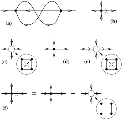
Figure 5: (a) The same diagram as in Fig. 2c in the “thin-line” notation. (b) Differentiation $\partial_{t}{\cal D}^{(0)}_{\eta}(t)$. (c) Vertex with $(\varphi_{i}-\varphi_{j})^{2}$ terms. At the vertex, the solid/dashed lines denote $a_{ij}=\pm 1$ respectively, cf. Eq. (160). (d) Contraction of the diffuson: ${\cal D}^{(0)}_{\eta}(t)$ is replaced by $\delta(t)$. (e) An original vertex of the sigma-model action (four-valent vertex is shown as an example). The differentiations $\hat{\partial}$ and $a_{ij}(\varphi_{i}-\varphi_{j})^{2}$ terms are added together. (f) Graphical presentation of the diffuson equation of motion (38): $\partial_{t}{\cal D}^{(0)}_{\eta}(t)=\delta(t)-\eta^{2}{\cal D}^{(0)}_{\eta}(t)$ (with $\alpha$ set to 1).

In this Appendix, to simplify the figures, we shall pictorially denote the diffusons by single lines (with arrows), instead of double lines as in Figs. 1 and 2. The order of the arrows at any vertex remains important: it represents the order of $b$-operators in the corresponding product $\mathop{\rm Tr}\nolimits(b{\bar{b}}b\dots\bar{b})$. In particular, arrows going to/from any vertex alternate between incoming and outgoing directions. Only vertices of even order are allowed. The diagram from Fig. 2c is again shown in Fig. 5a in the new notation. The vertices may contain differentiations represented by a cross (Fig. 5b) and $(\varphi_{i}-\varphi_{j})^{2}$ terms (Fig. 5c). When we transform a diffuson according to the equation of motion (38), there appear terms with the diffusons replaced by the $\delta$-function. Such a replacement will be denoted further as the double-crossed diffuson, Fig. 5d.

Before turning to canceling vertices, we calculate the numerical prefactors at each diagram. For simplicity, we perform now the calculation only for diagrams representing corrections to the pro-diffuson (33) defined as the $\langle b{\bar{b}}\rangle$ propagator, with one incoming and one outgoing diffusons. Let $N_{D}$ denote the number of diffusons, $N_{V}$ the number of vertices, and $2n_{i}$ be the vertex valencies. Then $N_{D}=1+\sum n_{i}$ and the number of loops in the diagram is $L=N_{D}-N_{V}-1$.

Every diffuson in the diagram brings in an additional factor of $(2/\pi)$. In the rational parameterization (29), collecting the coefficients of the vertices $S_{\rm E}^{(\geq 4)}$ [Eq. (25)] and $S_{\rm kin}^{(\geq 4)}$ [Eqs. (26) and (30)] (and taking into account the $n_{i}$-fold symmetry of vertices (26)), the total numerical prefactor in front of the diagram for the pro-diffuson ${\cal D}^{*}=(\pi/2)\langle b\bar{b}\rangle$ [Eq. (33)] becomes $(-1)^{N_{D}-1}(2\pi)^{-L}$. With this prefactor, each vertex coming from $S_{\rm E}^{(\geq 4)}$ enters with the coefficient 1, and each vertex originating from $S_{\rm kin}^{(\geq 4)}$ enters with the coefficient $\alpha a_{ij}$, where

$$a_{ij}=(-1)^{i-j+1}.$$ (160)

Finally, by rescaling the time in the units of $\alpha^{-1/3}$, the diagram acquires the overall factor $\alpha^{-L/3}$ ($\alpha^{1/3}$ for every vertex and $\alpha^{-(N_{D}-1)/3}$ from $N_{D}-1$ independent time integrations). Now we may factor out the common coefficient for all the diagrams of a given order $L$, and the remaining coefficients equal plus or minus one. Note that within a given order $L$, the relative sign alternates between diagrams with different number of vertices.

Figure 6: (a) Tree-like graph of contracted diffusons. (b) Loop of contracted diffusons.

The diagrammatic rules now may be formulated as follows.

1. First we draw all the diagrams of a given order $L$ allowed by the no-loop rule (see Section III). The sign of the diagram is $(-1)^{N_{D}-1}$.

2. In every vertex, we put the sum of all differentiations on outgoing diffusons ($S_{\rm E}$-generated) and the full graph of $a_{ij}(\varphi_{i}-\varphi_{j})^{2}$ ($S_{\rm kin}$-generated), see Fig. 5e.

3. We expand every differentiation according to the diffuson equation of motion (Fig. 5f).

4. During this differentiation, some of the diffusons are replaced by $\delta$ functions, which leads to merging or splitting some vertices (discussed in details below). Since every vertex has at most one differentiation on outgoing diffusons, the connected graph of “contracted” diffusons contain no more than one loop. We further distinguish two possibilities:

   • the connected graph of “contracted” diffusons is a tree (contains no loops), Fig. 6a. In this case, all the vertices of the graph are contracted to a single vertex (“root” of the tree; point $A$ in Fig. 6a). As the result of summing such diagrams, the coefficients $a_{ij}$ at the “root” vertex get modified.

   • the connected graph of “contracted” diffusons contains one loop, Fig. 6b. Then upon contraction, we obtain two disconnected vertices without any $(\varphi_{i}-\varphi_{j})^{2}$ factors (vertices of this type would also be generated by the Jacobian action as described in Appendix B, if the Jacobian were not equal to one).

   In the subsequent subsections we sum separately those two series of diagrams and show that in the case (i) vertices of order higher than four cancel, and in the case (ii) all such loop-contractions cancel each other.

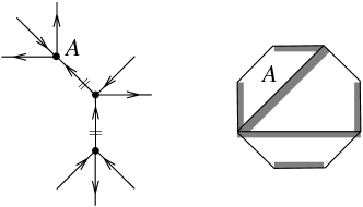
Figure 7: An example of a contraction tree and the corresponding polygon (room-painting) diagram.

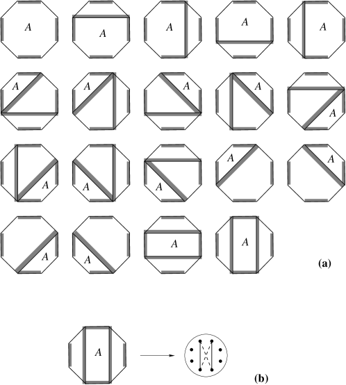
Figure 8: (a) All admissible room partitions of the 8-wall room. (b) Every partition contributes the full graph of the “distinguished” room $A$ minus the external painted walls (and the whole graph is multiplied by $(-1)$ to the number of internal walls).

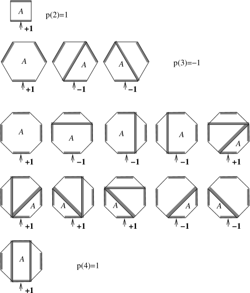
Figure 9: An example of a direct enumeration of $p(2)$, $p(3)$, $p(4)$.

C.2 Cancellations in tree-like contractions

Consider now the case when the connected graph of contracted diffusons is a tree (Fig. 6a). This tree has one distinguished vertex (denote it $A$) which does not contain differentiation. All the $(\varphi_{i}-\varphi_{j})^{2}$ terms of the resulting “contracted” vertex come from the vertex $A$. Now we represent the contracted vertex as a $2n$-polygon, and the possible graph configurations leading to this vertex as dividing this polygons by several diagonals into smaller polygons (Fig. 7). Each such diagonal (a “separator”) should be thought of as a “wall” which represents a diffuson to be contracted. We “paint” such a wall from the side of the $b$-operator (the side of differentiation). The “outside” walls of the big $2n$-polygon are also originally painted in the alternating order (Fig. 7). With this representation, the different contractible graphs generating a given vertex are in one-to-one correspondence with “admissible” partitions of $2n$-polygons into smaller “rooms”. A partition is called “admissible” if after painting all the walls in alternating order, no room has more than one painted separator. Obviously, with this rule, exactly one room of the partition has no painted separator. This room is called the “distinguished” room of the partition. As an illustration, in Fig. 8a we show all the admissible partitions of the 8-wall room. From our discussion of the diagram rules and prefactors, each partition contributes to the contracted vertex the “full graph of the distinguished room” minus “painted walls of the distinguished room” with the relative sign of the parity number of rooms in the partition. Here the “full graph” means the full graph with the sign $\sum(-1)^{i-j+1}(\varphi_{i}-\varphi_{j})^{2}$, and the painted walls are subtracted when expanding the corresponding differentiations (see fig. 8b for an example).

Before we compute the total vertex as a sum of all room partitions, we define a combinatoric quantity $p(n)$. Consider a $2n$-wall room with external walls painted in the alternating order, and one of the painted walls is “special” (say, it has a door). Let $p(n)$ denote the “algebraic” number of all admissible partitions of the $2n$-room such that the distinguished room contains special wall. By the “algebraic” number we mean that every partition comes with plus or minus sign depending on the parity of the rooms in the partition (and the trivial partition with only one room comes with plus sign). For example, $p(2)=1$, $p(3)=-1$, $p(4)=1$ (Fig. 9), etc.

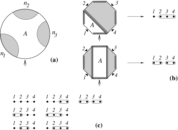
Figure 10: (a) A schematic picture of external blocks adjacent to the “distinguished” room A. (b) Combinatoric diagrams representing the external block configurations. (c) All possible external block configurations in computing $p(4)$.

One can prove by induction that $p(n)=(-1)^{n}$. Indeed, all partitions may be classified by “external” blocks (shaded in fig. 10a) adjacent to the distinguished room. Each of those external blocks contributes $-p(n_{i})$ possibilities to subdivide it, where $n_{i}$ is the number of unpainted external walls of the block. All possible configurations of external blocks may be enumerated by dividing the total of $n$ unpainted external walls into non-intersecting sequences of length $n_{i}$. Thus,

$$p(n)=\sum\prod(-p(n_{i})),$$ (161)

where the sum is taken over all possibilities to choose a set of non-intersecting blocks of adjacent elements from a sequence of total $n$ elements (Fig. 10b). The only element excluded from the sum is the set where the whole sequence belongs to a single block. In Fig. 10c we illustrate the possible choices of such block sets for $n=4$. Now we perform the induction step assuming that for all $n_{i}<n$, $p(n_{i})=(-1)^{n_{i}}$. Then the same sum (161) may be rewritten as $p(n)=\sum(-1)^{n_{\rm adj}}$, where $n_{\rm adj}$ is the number of adjacent pairs belonging to the same block. Finally, we note that we may parameterize block sets by independently choosing two neighboring elements either to belong or not to belong to the same block. This easily gives us the total sum. If all the sets were allowed, the sum would be zero. The only set which is not allowed is the one with all neighboring elements (total $n-1$ pairs) belonging to the same block. This gives $p(n)=(-1)^{n}$, which completes the proof.

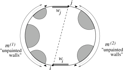
Figure 11: The painted walls $w_{i}$ and $w_{j}$ divide the boundary into two pieces of lengths $m^{(1)}$ and $m^{(2)}$.

Now we do the final step of the calculation: we calculate the renormalized coefficient $\tilde{a}_{ij}$ with which the combination $(\varphi_{i}-\varphi_{j})^{2}$ enters the contracted vertex. First, such terms with $i$ adjacent to $j$ through a painted external wall never enter (they are always subtracted by expanding differentiations). So we may assume that $i$ and $j$ belong to different painted external walls (let us call those walls $w_{i}$ and $w_{j}$ for future reference).

A room partition gives a contribution to $\tilde{a}_{ij}$ if and only if $w_{i}$ and $w_{j}$ both belong to the distinguished room. Similarly to our discussion above, for each room partition, we may consider external “blocks” complementary to the distinguished room. Now the walls $w_{i}$ and $w_{j}$ divide the unpainted walls into two sequences (define their lengths as $m^{(1)}$ and $m^{(2)}$), and the contributions from these two sequences factorize:

$$a_{ij}=(-1)^{i-j-1}\sum_{(1)}\prod(-p(m^{(1)}_{i}))\sum_{(2)}\prod(-p(m^{(2)}_{i}))$$ (162)

(see Fig. 11). The only difference from the previous calculation is that now the whole sequence $m^{(1)}$ (or $m^{(2)}$) is allowed to be placed in one block. Therefore the sum gives zero unless both $m^{(1)}$ and $m^{(2)}$ equal one. But this is possible only if the total number of unpainted external walls is $n=m^{(1)}+m^{(2)}=2$, i.e. for the four-valent vertex. This completes the proof that all higher-order vertices cancel in the process of tree-like contractions.

The only surviving four-leg vertex is shown in Fig. 12, with

$$\sum_{i<j}\tilde{a}_{ij}(\varphi_{i}-\varphi_{j})^{2}=(\varphi_{2}-\varphi_{3})^{2}+(\varphi_{1}-\varphi_{4})^{2}-(\varphi_{1}-\varphi_{3})^{2}-(\varphi_{2}-\varphi_{4})^{2}=2(\varphi_{1}-\varphi_{2})(\varphi_{3}-\varphi_{4}).$$ (163)

The diagrammatic series with such a vertex may be considered as a perturbative expansion of the field theory (39), (40).

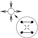
Figure 12: The resulting four-valent vertex.

C.3 Cancellation of loop-like contractions

In this section we prove cancellation of vertices obtained in the process of contracting a connected graph of diffusons containing a closed loop (Fig. 6b). After such a contraction, two vertices appear without any $(\phi_{i}-\phi_{j})^{2}$ terms. This is the same type of vertices as those appearing from the Jacobian. We consider the rational parameterization which contains no Jacobian vertices, so the only vertices of this type are those produced by the closed-loop diffuson contractions.

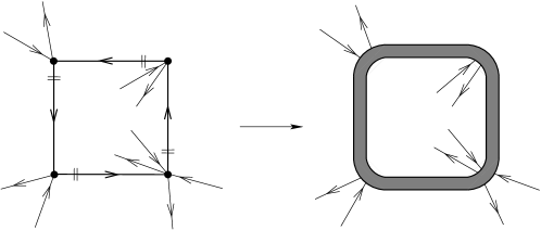
Figure 13: The loop contraction of diffusons. The inner and outer boundaries of the shaded region in the right-hand side are contracted into two separate vertices.

Here we make two important remarks. First, there is no internal structure of those vertices, and the only parameter of the vertex is its numerical prefactor. Second, it is sufficient to prove cancellation of the “loop part” of the diagram (Fig. 13) containing only the closed loop of contracted diffusons, without any “branches” which do not depend on the internal structure of the loop part.

So we consider loops of length $l\geq 1$ of contracted diffusons. If we go along the loop, the legs on the left and on the right sides of our path are collected into two new “contracted” vertices. We fix the valencies of these vertices to be $2n$ and $2m$ and count the total combinatoric factor $p(n,m)$ as the number of ways to obtain these vertices from loops of different lengths. Taking into account the sign alternating with the total vertex number, we obtain

$$p(n,m)=\sum_{l=1}^{\infty}(-1)^{l}p_{l}(n,m),$$ (164)

where $p_{l}(n,m)$ is the positive integer number counting the number of ways to create the two vertices of valencies $2n$ and $2m$ from the loop of length $l$. Note that from the left-right hand rule both $n$ and $m$ must be positive. Also, since the two-leg vertices are not allowed in the original action, $p_{l}(n,m)=0$ for $l>n+m$. An example of calculating $p(1,2)$ is shown in Fig. 14.

Figure 14: Direct computation of $p(1,2)=-p_{1}(1,2)+p_{2}(2,2)-p_{3}(1,2)=0$.

The combinatoric problem of computing $p_{l}(n,m)$ may be related to computing another combinatoric quantity $q_{l}(n,m)$ defined as the number of ways to distribute $n$ identical black and $m$ identical white balls among $l$ different boxes so that no box remains empty:

$$p_{l}(n,m)=nm\frac{1}{l}q_{l}(n,m)$$ (165)

(here factors $n$ and $m$ come from different ways to circularly re-label external legs, and $1/l$ factors reflects equivalence of diagrams obtained by the circular permutation of vertices). The example of calculating $q_{l}(1,2)$ is shown in Fig. 15.

Figure 15: Example of $q_{l}(n,m)$ definition: direct computation of $q_{l}(1,2)$.

Finally, we use the generating-function method to compute $q_{l}(n,m)$. Consider the series

$$f_{l}(x,y)=(x+y+x^{2}+xy+y^{2}+\dots)^{l},$$ (166)

where the expression in the brackets contains all terms $x^{n_{x}}y^{n_{y}}$ except for $n_{x}=n_{y}=0$. Then the coefficient at $x^{n}y^{m}$ in the Taylor expansion of $f(x,y)$ equals $q_{l}(n,m)$. Now a straightforward calculation gives:

$$f_{l}(x,y)=\left(\frac{1}{(1-x)(1-y)}-1\right)^{l},$$ (167)

and then

$$\sum_{l=1}^{\infty}\frac{1}{l}(-1)^{l}f_{l}(x,y)=\ln(1-x)+\ln(1-y)$$ (168)

(note the factorization!). Now the coefficient $p(n,m)$ equals $nm$ times the coefficient at $x^{n}y^{m}$ in the Taylor expansion of the expression (168). The latter however equals 0 unless one of the two numbers $n$ or $m$ is zero. This finishes the proof: all vertices generated from loop contractions cancel.

References

- (1) M. L. Mehta, Random Matrices and the Statistical Theory of Energy Levels (Academic, New York, 1991).
- (2) T. Guhr, A. Mueller-Groeling, H. A. Weidenmueller, Phys. Rep. 299, 189 (1998).
- (3) K. B. Efetov, Supersymmetry in Disorder and Chaos (Cambridge University Press, New York, 1997).
- (4) M. Wilkinson, J. Phys A 21, 4021 (1988).
- (5) B. D. Simons and B. L. Altshuler, Phys. Rev. Lett 70, 4063 (1993); Phys. Rev. B 48, 5422 (1993).
- (6) G. Casati, B. V. Chirikov, J. Ford, and F. M. Izrailev, in Stochastic Behaviour in Classical and Quantum Hamiltonian Systems, ed. by G. Casati and J. Ford, Lecture Notes in Physics, vol. 93 (Springer, Berlin, 1979).
- (7) M. Wilkinson and E. J. Austin, Phys. Rev. A 46, 64 (1992).
- (8) D. M. Basko, M. A. Skvortsov, and V. E. Kravtsov, Phys. Rev. Lett. 90, 096801 (2003).
- (9) M. A. Skvortsov, Phys. Rev. B 68, 041306(R) (2003).
- (10) M. A. Skvortsov, D. M. Basko, and V. E. Kravtsov, Pis ma v Zh. Eksp. Teor. Fiz. 80, 60 (2004) [JETP Lett. 80, 54 (2004)].
- (11) For the Gaussian Orthogonal Ensemble, the parameter is defined as , and .
- (12) F. J. Dyson, Phys. Rev. 102, 1217 (1956); 102, 1230 (1956).
- (13) S. V. Maleev, Zh. Eksp. Teor. Fiz. 33, 1010 (1957) [Sov. Phys. JETP 64, 654 (1958)].
- (14) F. Wegner, Z. Phys. B 35, 207 (1979).
- (15) K. B. Efetov, A.I. Larkin, D. E. Khmelnitskii, Zh. Eksp. Teor. Fiz. 79, 1120 (1980) [Sov. Phys. JETP 52, 568 (1980)].
- (16) A. Kamenev and A. Andreev, Phys. Rev. B 60, 2218 (1999).
- (17) M. L. Horbach and G. Schön, Ann. Phys. (Berlin) 2, 51 (1993).
- (18) A. Altland and A. Kamenev, Phys. Rev. Lett. 85, 5615 (2000).
- (19) K. B. Efetov, Adv. Phys. 32, 53 (1983).
- (20) Convergence of the diagrams for remains at the level of conjecture. We explicitly see that the diagrams are convergent in two- and four-loop calculations [integrals (44) in the four-loop case]. We do not have a proof of this conjecture at arbitrary order.
- (21) B. L. Altshuler, A. G. Aronov, and D. E. Khmelnitsky, J. Phys. C 15, 7367 (1982).
- (22) M. G. Vavilov and I. L. Aleiner, Phys. Rev. B 60, R16311 (1999).
- (23) J. Holstein and N. Primakoff, Phys. Rev. 58, 1908 (1940).
- (24) C. M. Canali, S. M. Girvin, and M. Wallin, Phys. Rev. B 45, 10131 (1992).
- (25) C. J. Hamer, Zheng Weihong, and P. Arndt, Phys. Rev. B 46, 6276 (1992); Zheng Weihong and C. J. Hamer, Phys. Rev. B 47, 7961 (1993).
- (26) I. V. Kolokolov, Pis ma v Zh. Eksp. Teor. Fiz. 72, 201 (2000) [JETP Lett. 72, 138 (2000)].
- (27) I. A. Gruzberg, N. Read, and S. Sachdev, Phys. Rev. B 56, 13218 (1997).
- (28) J. J. Duistermaat and G. Heckman, Inv. Math. 69, 259 (1982); 72, 153 (1983).
- (29) M. R. Zirnbauer, cond-mat/9903338 (unpublished).
- (30) J. Rammer and H. Smith, Rev. Mod. Phys. 58, 323 (1986).
- (31) In notations of Ref. skvor, inherited from Ref. KamenevAndreev99, , the lower-right block of was defined as . The two theories are trivially equivalent by the rotation of the unitary matrices in Eq. (11).
- (32) S. Hikami, Phys. Rev. B 24, 2671 (1981).
- (33) A. A. Abrikosov, L. P. Gorkov and I. E. Dzyaloshinskii, Methods of Quantum Field Theory in Statistical Physics (Dover, New York, 1975).
- (34) J. J. M. Verbaarschot and M. R. Zirnbauer, J. Phys. A 18, 1093 (1985).
- (35) I. V. Yurkevich and I. V. Lerner, Phys. Rev. B 60, 3955 (1999).