Measuring the kernel of time-dependent density functional theory with X-ray absorption spectroscopy of $3d$ transition metals

Abstract

The $2p-3d$ core hole interaction in the $L_{2,3}$ absorption spectra of the $3d$ transition metals is treated within time-dependent density functional theory (TDDFT). A simple three-level model explains the origin of the strong deviations from the one-particle branching ratio and yields matrix elements of the unknown exchange-correlation (XC) kernel directly from experiment.

Ground-state density functional theory (DFT) is well-established for atoms, molecules, and solids FNM03 . But ground-state DFT produces only a one-particle picture of the electronic transitions in matter, neglecting interactions between excitations. In the optical regime, time-dependent DFT (TDDFT) has enjoyed recent success PGG96 ; reining ; sole in describing such dynamic exchange-correlation (XC) effects. The spectroscopic properties of matter in the X-ray regime are substantially governed by dynamical many-body effects involving the creation of a localized core hole zaanen85 ; schwitalla ; shirley ; corerehr ; eriksson . While GW calculations and the Bethe-Salpeter equation can be used shirley , these are computationally demanding. The less expensive methodology of TDDFT is now being developed for these effects corerehr .

We analyze this approach to the X-ray absorption of itinerant systems like the $L_{2,3}$ absorption of $3d$ transition metals (TMs), i.e., exciting a photoelectron from the localized $2p$ core states into the $3d$ band. $L_{2,3}$ X-ray absorption spectra (XAS), especially of early $3d$ TMs, suffer from core-hole correlation effects zaanen85 . Schwitalla and Ebert schwitalla applied TDDFT linear response theory to calculate the XAS of the $3d$ TMs. Using a local approximation to the frequency-dependent XC kernel, as proposed by Gross and Kohn gross_kohn , they qualitatively reproduced the trend of the branching ratios. However, whenever DFT is applied in a new regime, a difficult question arises: Are the existing functional approximations sufficiently accurate in this new regime? And how does one separate XC errors from those due to the practical approximations needed for realistic calculations? In Ref. corerehr , the limitations of the Gross-Kohn approximation for this problem are shown, and a new approximation suggested. But the true value of DFT is in constructing one XC approximation that covers many situations, in order to build-in knowledge of the underlying physics. Other TDDFT approximations, such as Vignale-Kohn VK96 , would need to be inserted into their codes in order to be tested.

Our approach here is different, and is based on the philosophy of Ref. AGB03 . That work examined the TDDFT response when excitations are not strongly coupled to each other. A useful series was developed in the strength of the off-diagonal matrix elements, relative to the frequency shifts induced by diagonal terms. The leading term yields the single-pole approximation (SPA)PGG96 , which has proven very useful in understanding TDDFT corrections to the one-particle picture. It even yields an immediate estimate of the XC kernel, but only if excitations are well-separated, a criterion rarely realized in practice AGB03 ; chelikowsky .

However, the same philosophy applies to cases of two levels strongly coupled to one another, but weakly coupled to the rest of the spectrum. We call this the three-level or double-pole approximation (DPA), cf. Fig 1. Moreover, the $L_{2,3}$ absorption of $3d$ TMs provides an ideal example of two transitions much closer to each other than the rest of the spectrum. With this in mind, we experimentally measured the branching ratios and level splittings of the $2p_{3/2}$($L_{3}$) and $2p_{1/2}$($L_{2}$) core states, and now deduce off-diagonal matrix elements of the unknown XC kernel. Because we can also compare with the one-particle Kohn-Sham (KS) spectrum, we can also deduce the diagonal matrix elements. The large deviation of branching ratios from their single-particle values is due entirely to the effect of core-hole interaction on spin-orbit coupling. Thus the DPA to TDDFT explains the observed shifts and oscillator strengths, and also provide benchmarks for future XC kernel approximations. We believe this is the first experimental measurement of a matrix element of the XC kernel of TDDFT.

Consider a system of electrons subject to a small frequency-dependent perturbation. By virtue of TDDFT the corresponding linear density-density response function $\chi$ is related to the response function $\chi_{s}$ of non-interacting particles via the Dyson-type equation gross_kohn

$$\chi(\mathbf{r},\mathbf{r}^{\prime},\omega)=\chi_{s}(\mathbf{r},\mathbf{r}^{\prime},\omega)$$ (1)

$$+\int\mbox{d}^{3}x\int\mbox{d}^{3}x^{\prime}\chi_{s}(\mathbf{r},\mathbf{x},\omega)K(\mathbf{x},\mathbf{x}^{\prime},\omega)\chi(\mathbf{x}^{\prime},\mathbf{r}^{\prime},\omega).$$

The kernel $K(\mathbf{r},\mathbf{r}^{\;\prime},\omega)$ consists of the bare Coulomb interaction and the frequency-dependent XC kernel $f_{xc}(\mathbf{r},\mathbf{r}^{\;\prime},\omega)$:

$$K(\mathbf{r},\mathbf{r}^{\prime},\omega)=\frac{e^{2}}{\left|\mathbf{r}-\mathbf{r}^{\prime}\right|}+f_{xc}(\mathbf{r},\mathbf{r}^{\prime},\omega).$$ (2)

The exact XC kernel describes, among other many-body effects, the core-hole interaction with the photoelectron. Neglecting $K$, the spectrum would reduce to the bare KS single particle spectrum represented by $\chi_{s}$. In XAS, the deviations produced by $K$ are called core-hole correlation effects. The response function $\chi_{s}$ is given in terms of the ground-state KS orbitals $\varphi_{j}$ (spin-saturated) by

$$\chi_{s}(\mathbf{r},\mathbf{r}^{\prime},\omega)=2\sum_{j,k}(n_{j}-n_{k})\frac{\varphi^{\ast}_{k}(\mathbf{r})\varphi^{\ast}_{j}(\mathbf{r}^{\prime})\varphi_{j}(\mathbf{r})\varphi_{k}(\mathbf{r}^{\prime})}{\omega-\omega_{jk}+i\eta}$$ (3)

where $n_{j},n_{k}$ denote the Fermi-occupation factors and $\omega_{jk}$ are the KS orbital-energy differences. For a single-particle transition $q$ ($q\equiv k\to j$) define $\Phi_{q}(\mathbf{r}):=\varphi_{k}(\mathbf{r})\varphi_{j}^{\ast}(\mathbf{r})$. The exact density-response function $\chi$ has poles at the true, correlated, excitation energies $\Omega_{j}$, which can be found by solving C96 :

$$\sum_{q^{\prime}}{\tilde{W}}_{qq^{\prime}}(\Omega_{j})\ v_{q^{\prime},j}=\Omega^{2}_{j}\ v_{q,j},$$ (4)

where the matrix is

$${\tilde{W}}_{qq^{\prime}}(\Omega) = \omega^{2}_{q}\,\delta_{qq^{\prime}}+4{\sqrt{\omega_{q}\,\omega_{q}^{\prime}}}\,K_{qq^{\prime}}(\Omega),$$

$$K_{qq^{\prime}}(\Omega) = \int d^{3}r\int d^{3}r^{\prime}\,\Phi^{*}_{q}({\bf r})\,K({\bf r}{\bf r}^{\prime}\Omega)\,\Phi_{q^{\prime}}({\bf r}^{\prime}).$$ (5)

The eigenvectors yield the oscillator strengthsC96 via

$$f_{j}=\frac{2}{3}\,|\vec{x}^{T}\,S^{-\frac{1}{2}}\,\vec{v}_{j}|^{2},$$ (6)

where $S^{-\frac{1}{2}}_{qq^{\prime}}=\delta_{qq^{\prime}}\;\sqrt{\omega_{q}}$ and $x_{q}$ is a column of the KS dipole matrix elements. This eigenvalue problem rigorously determines the excitation spectrum of the interacting system, but the quality of the results in any practical calculation depends crucially on the approximation employed for the XC kernel.

Figure 1: Schematic illustration of the DPA model. The model describes the shifts of the excitation energies (uncorrelated $\omega_{i}$ and correlated $\Omega_{i}$) and the changes in corresponding oscillator strengths $f_{i}$ in the presence of an excited core hole.

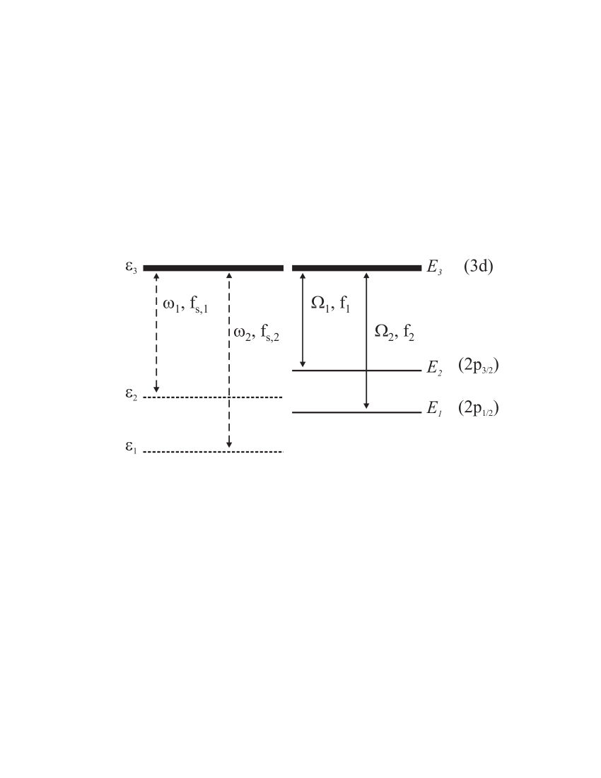
In the $L_{2,3}$ XAS of the $3d$ TMs, the description of the electron core-hole interaction may be simplified by the assumption that the relativistic spin-orbit coupling (SOC) in the $3d$ band states ($\sim 0.05$ eV) is small compared to that of the core states (several eV) and can be neglected. This means that the oscillator strengths $f_{j}$ of these levels are all about equal, as their KS orbitals are essentially identical. Since, in this limit, the absorption area is proportional to the oscillator strength, weighted statistically according to the manifold of the $j=3/2$ and $j=1/2$ subshells, the branching ratio of the KS system is $B_{\mathrm{KS}}=A_{3/2}/(A_{3/2}+A_{1/2})\equiv 2/3$, where $A_{j}$ is the area under the peak of the $j$-th subshell. (Ab initio calculations of the $L_{2,3}$ XAS without core-hole correlation effects based on the fully-relativistic spin-polarized Korringa-Kohn-Rostoker band structure formalism yield branching ratios very close to $B_{\mathrm{KS}}$ v-paper ; xafs12 .) Here we replace all dipole-allowed transitions $\omega_{jk}$ from a particular absorption edge into the $3d$ band by a single particle transition, as illustrated in Fig. 1.

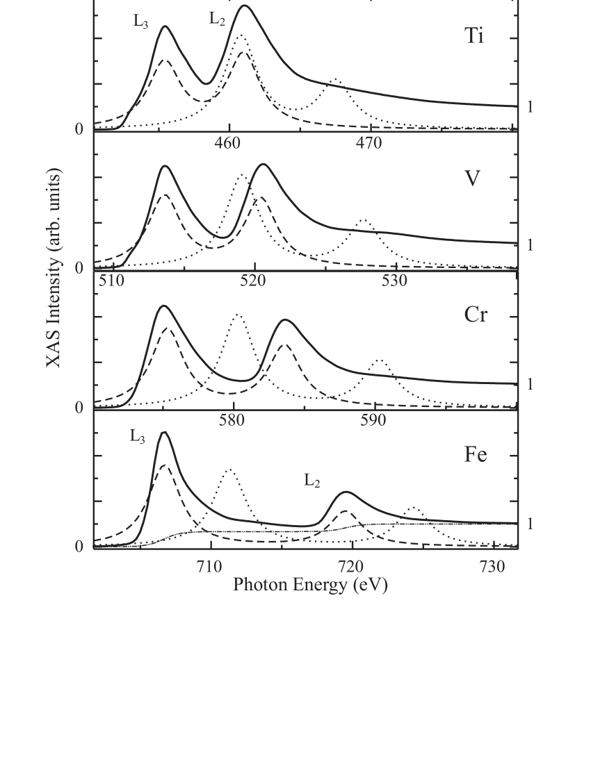
In Fig. 2, we show our experimental isotropic XAS for the $3d$ TM with almost empty $3d$ bands taken from Fe/TM/Fe sandwiches with $\mathrm{TM}=\mathrm{Ti,V,Cr}$ and bulk-like Fe. The data were recorded at the UE56-1/PGM beamline at BESSY (for details, see Ref. xafs12 ). The edge jumps are normalized to unity. From these spectra and their absolute energy dependence, the excitation energies $\Omega_{q=1}$ at the $L_{3}$ edge and $\Omega_{q=2}$ and the $L_{2}$ edge are determined. For the quantitative analysis of the branching ratio $B$, we very carefully determined the $L_{2,3}$ absorption areas $A_{j}$. This determination has the advantage that $B$ becomes independent of the different $L_{3}$ and $L_{2}$ lifetime broadening and experimental resolution. Note, that the proper experimental intensity is given by the area and not by the height of the resonance. To determine the correct area of the $L_{3}$ and $L_{2}$ resonances the continuum contribution is removed (e.g. gray line for Fe in Fig. 2 chenprl ). Since the $2p$ SOC decreases towards lower atomic numbers the deconvolution is more complicated for the early $3d$ TMs Ti, V, and Cr because of the strong $L_{2,3}$ overlap. The areas have been fitted using the Fe absorption spectrum as a background simulation underneath the $L_{2}$ edge. This fit appears justified, since the $L_{2}$ onsets for the early $3d$ TMs follow systematically the energy dependence of the $L_{3}$ edge of Fe. The experimental results are set out in Table 1. The energy resolution of the experimental spectra (Fig. 2) is approximately 0.5 eV. Consequently, the widths of a few eV in the $L_{3}$ and $L_{2}$ resonances are mostly due to lifetime effects.

In the case of Fe the $L_{2}$ absorption is approximately half of the $L_{3}$ peak, in agreement with the KS prediction. However, the branching ratios for the other $3d$ elements differ significantly from this. In particular, Ti has an $L_{2}$ peak that is even larger than its $L_{3}$ absorption. Thus, the experimental branching ratios cannot be interpreted in terms of KS orbitals, suggesting strong electron core-hole interactions. In the language of TDDFT, there must be significant off-diagonal matrix elements in Casida’s equations, describing the influence of the electron core-hole interaction on the $L_{2,3}$ XAS. (If only diagonal elements are considered in Eq. (4), the eigenvalues are shifted but the eigenvectors are not rotated, and the oscillator strengths retain their KS values AGB03 .)

Figure 2: The experimental isotropic absorption spectra (solid line) at the $L_{2,3}$ edges are shown for the early $3d$ TMs Ti, V, and Cr versus Fe. The edge jumps are normalized to unity for direct comparison. The continuum in the experimental spectrum is simulated by a two-step function as shown for Fe (dashed-dotted line). The treatment of the core hole red-shifts the independent particle spectrum (dotted line) and changes the statistical branching ratio in the correlated spectrum (dashed line) as revealed by the DPA model.

However, a fully numerical solution of the equations is not needed, as we know there are only two dominant transitions, so the electron core-hole interaction can be analyzed within the DPA model. For only two transitions, we solve Eq. (4) exactly:

$$f_{1} = ({\sqrt{f_{{\scriptscriptstyle\rm S},1}}}\;\cos(\theta/2)-{\sqrt{f_{{\scriptscriptstyle\rm S},2}}}\;\sin(\theta/2))^{2}$$

$$f_{2} = ({\sqrt{f_{{\scriptscriptstyle\rm S},2}}}\;\cos(\theta/2)+{\sqrt{f_{{\scriptscriptstyle\rm S},1}}}\;\sin(\theta/2))^{2}$$ (7)

for the interacting oscillator strengths $f_{i}$, where

$$\tan\theta=2\,W_{12}/(W_{22}-W_{11})$$ (8)

is a mixing angle that represents the strength of the coupling between the two transitions. This yields:

$$\cos\theta=\frac{4{\sqrt{f_{\scriptscriptstyle\rm S,1}f_{\scriptscriptstyle\rm S,2}q_{1}q_{2}}}+(f_{\scriptscriptstyle\rm S,2}-f_{\scriptscriptstyle\rm S,1})(q_{2}-q_{1})}{(f_{\scriptscriptstyle\rm S,1}+f_{\scriptscriptstyle\rm S,2})(q_{1}+q_{2})}$$ (9)

where $f_{\scriptscriptstyle\rm S,i}$ denotes a Kohn-Sham oscillator strength and $q_{1}=Bp_{2}$, $q_{2}=(1-B)p_{1}$, where $p_{i}$ the multiplicity of the initial state of transition $i$. In our case, setting $f_{{\scriptscriptstyle\rm S},1}=f_{{\scriptscriptstyle\rm S},2}=f_{0}$, Eq. (7) simplifies to

$$f_{1}=f_{0}\;(1-\sin\theta),~{}~{}~{}~{}~{}f_{2}=f_{0}\;(1+\sin\theta),$$ (10)

and since the absorption depends only on the oscillator strengths, weighted statistically, Eq. (9) yields

$$\sin\theta=(2-3B)/(2-B).$$ (11)

The branching ratio directly determines the mixing angle! We can even extract directly the off-diagonal matrix element of the Hartree-XC kernel itself. Inserting the matrix elements into Eq. (8), and neglecting all small differences (e.g., between KS and exact transition frequencies) which are a few eV in several hundred,

$$K_{12}=\sin\theta\;\Delta\Omega/4\;.$$ (12)

Thus knowledge of both the branching ratio and the level splitting $\Delta\Omega=\Omega_{2}-\Omega_{1}$ yields an experimental determination of the off-diagonal matrix element of the XC kernel. Lastly, given the ground-state KS energy levels, we can also recover the diagonal elements:

$$K_{jj}=(\Omega_{1}+\Omega_{2})/4+(-1)^{j}\Delta\Omega\;\cos\theta\;/4-\omega_{j}/2\;\quad j=1,2.$$ (13)

These results are listed in Table 1, the corresponding theoretical DPA spectra are presented in Fig. 2.

This analysis yields a simple interpretation of the observed spectra. First, imagine there was no SOC. Then there would be a single $p$-level, and SPA applies. The diagonal matrix element of $f_{\scriptscriptstyle\rm HXC}$ is the well-known core-hole interaction that shifts the transition frequency from its KS value. In the presence of spin-orbit splitting, both levels are shifted by similar amounts, about 5-7 eV.

Much more importantly, a new effect occurs, which is that the core-hole interaction couples the two KS transitions together, altering their branching ratio. The much smaller off-diagonal core-hole interaction (about 1/2 eV) produces the large deviation from the single-particle branching ratio. Although the matrix elements are about 5 times smaller than their diagonal counterparts, in Ti they reverse the relative sizes of the peaks. This effect can be thought of as simple level (or in this case, transition) repulsion, as the two transitions near one another. Eq. (12) shows that the true measure of coupling is $4|K_{12}|/\Delta\Omega$, which is growing from Fe to Ti only because the $2p$ SOC $\Delta\Omega$ is shrinking, not because of increased interaction. We also note that SPA PGG96 (which can be recovered in all results by setting $\theta=0$) yields $2K_{jj}=\Omega_{j}-\omega_{j}$ and is highly accurate for the diagonal elements. Thus the shifts are simply interpreted as diagonals of $K$, while the branching ratios are a sensitive determinant of off-diagonal elements. Lastly, for very small splitting ($\Delta\Omega\ll 4K_{12}$), $\sin\theta\to 1$ and, from Eq. (7), all weight goes into the $L_{2}$ peak. From Eqs.(12-13):

$$\Delta\Omega=2\sqrt{(\Delta\omega/2+K_{22}-K_{11})^{2}+4K_{12}^{2}}\;.$$ (14)

Thus $4|K_{12}|$ is the minimum level splitting, and occurs with the $L_{2}$ peak much larger than $L_{3}$.

The success of DPA shows that very little effort beyond a ground-state DFT calculation is needed to compute these spectra in TDDFT. One only needs to integrate a given approximation to the XC kernel for the two diagonal matrix elements, and one off-diagonal. Furthermore, applying our analysis in reverse to the calculated ALDA and RPA results of Fig. 1 of Ref. corerehr , we find that the success of the suggested approximation (which implies using ALDA for diagonal elements, and neglecting XC for the off-diagonal elements, i.e., RPA) also implies that ALDA is accurate for the peak shifts alone, while RPA is accurate for the branching ratio predicted by Eq. (12), once the experimental shift is used.

Why is DPA justified for these systems? There are two clear sources of error. On the one hand, there are transitions to other levels to consider, but these are well-known to have small effects W04 . For example, the transitions to $4s$ have much smaller oscillator strengths, while other transitions are included in the background, which has been subtracted. Of greater concern might be the lack of resolution of the (slightly) split $3d$ levels, which yield a 9$\times$9 Casida matrix problem of allowed transitions. However, just as DPA reduces to the single-pole approximation of Ref. AGB03 when levels are too close to be resolved AGB06 , we expect the full solution of the 9$\times$9 problem to collapse to the DPA results when the individual $d$-levels cannot be resolved. This will only be true for the early TM’s, in which most of the $3d$-levels are unoccupied.

Table 1: Excitation energies in eV obtained from KS calculations ($\omega_{i}^{KS}$) and from experiment ($\Omega_{i}$), experimental branching ratio $B$ and matrix elements $K_{ij}$. The experimental error of $\Omega_{i}$ is below $10^{-3}$, the one of $B$ in the order of 1 %.

$3d$ TM	$\omega_{1}^{KS}$	$\omega_{2}^{KS}$	$\Omega_{1}$	$\Omega_{2}$	$B$	$K_{11}$	$K_{22}$	$K_{12}$
22 Ti	460.8	467.5	455.4	461.0	0.47	-2.57	-3.34	0.54
23 V	519.1	527.7	513.6	520.4	0.51	-2.65	-3.73	0.54
24 Cr	580.3	590.3	575.1	583.6	0.56	-2.55	-3.40	0.47
26 Fe	711.3	724.6	706.7	719.5	0.70	-2.29	-2.55	-0.25

In summary, we have used TDDFT to understand the XAS of $3d$ transition metals by deriving a double-pole approximation. The main features observed in the experiments can easily be explained by assuming that the spectrum is dominated by two strongly coupled poles via the $2p-3d$ core hole interaction. This shows that, for the beginning of the $3d$ series, the reduced $2p$-SOC is responsible for the strong variation of the branching ratio, not strong interactions between the transitions. Our analysis does not replace a full TDDFT calculation of X-ray absorption spectra. Rather, for the very specific case of spectral regions dominated by two poles it provides, on the one hand, a transparent picture of the changes of spectral weights in particular for the early $3d$ TMs, and on the other, a straight-forward route to testing approximate XC kernels against experimental data.

Discussions with J. J. Rehr and U. Diebold are acknowledged. We also thank the authors of Ref. corerehr for their KS eigenvalues. The work was supported by BMBF (05 KS4 KEB/5) and DFG, Sfb 290. Partial financial support by the EXC!TING Research and Training Network of the EU and the NANOQUANTA network of excellence is gratefully acknowledged. KB thanks the US DOE (DE-FG02-01ER45928) and NSF (CHE-0355405).

References

- (1) A Primer in Density Functional Theory, ed. C. Fiolhais, F. Nogueira, and M. Marques (Springer-Verlag, NY, 2003).
- (2) M. Petersilka, U.J. Gossmann, E.K.U. Gross, Phys. Rev. Lett. 76, 1212 (1996).
- (3) F. Sottile, V. Olevano, and L. Reining, Phys. Rev. Lett. 91, 056402 (2003).
- (4) A. Marini, R. Del Sole, and A. Rubio, Phys. Rev. Lett. 91, 256402 (2003)
- (5) J. Fink et al., Phys. Rev. B 32, 4899 (1985); J. Zaanen, et al., ibid. 32, 4905 (1985).
- (6) J. Schwitalla and H. Ebert, Phys. Rev. Lett. 80, 4586 (1998).
- (7) E.L. Shirley, Phys. Rev. Lett. 80, 794 (1998).
- (8) A.L. Ankudinov, A.I. Nesvizhskii, and J.J. Rehr, Phys. Rev. B 67, 115120 (2003).
- (9) O. Wessely, M.I. Katsnelson, and O. Eriksson, Phys. Rev. Lett. 94, 167401 (2005).
- (10) E.K.U. Gross and W. Kohn, Phys. Rev. Lett. 55, 2850 (1985).
- (11) G. Vignale and W. Kohn, Phys. Rev. Lett. 77, 2037 (1996).
- (12) H. Appel, E.K.U.Gross, and K. Burke, Phys. Rev. Lett. 90, 043005 (2003) and erratum in preparation.
- (13) I. Vasiliev et al., Phys. Rev. Lett. 82, 1919 (1999).
- (14) M.E. Casida, in Recent developments and applications in density functional theory, ed. J.M. Seminario (Elsevier, Amsterdam, 1996).
- (15) A. Scherz et al., Phys. Rev. B 66, 184401 (2002).
- (16) A. Scherz et al., Physica Scripta T115, 586 (2005).
- (17) C.T. Chen et al., Phys. Rev. Lett. 75, 152 (1995).
- (18) H. Wende, Rep. Prog. Phys. 67, 2105-2181 (2004).
- (19) H. Appel, E.K.U. Gross, and K. Burke, cond-mat/0504436.