Theory of infrared conductivity and Hall conductivity Based on the
Fermi Liquid Theory: analysis of high-$T_{\rm c}$ superconductors

Abstract

We study optical conductivities for high-$T_{\rm c}$ superconductors under the magnetic field on the basis of the microscopic Fermi liquid theory. Current vertex corrections (CVC’s) are correctly taken into account to satisfy the conservation laws, which has been performed for the first time for optical conductivities based on the fluctuation-exchange (FLEX) approximation. We find that the CVC emphasizes the ${\omega}$-dependence of ${\sigma}_{xy}({\omega})$ significantly when the antiferromagnetic (AF) fluctuations are strong. By this reason, the relation ${\sigma}_{xy}({\omega})\sim\{{\sigma}({\omega})\}^{2}$, which is satisfied in the extended-Drude model given by the relaxation time approximation (RTA), is totally violated for a wide range of frequencies. Consequently, the optical Hall coefficient $R_{\rm H}({\omega})$ strongly depends on ${\omega}$ below the infrared frequencies, which is consistent with experimental observations. We also study the mystery about a simple-Drude form of the optical Hall angle $\theta_{\rm H}({\omega})$ observed by Drew et al., which is highly nontrivial in terms of the RTA since the strong ${\omega}$-dependence of the relaxation time should modify the Drude-form. We find that a simple Drude-form of $\theta_{\rm H}({\omega})$ is realized because the ${\omega}$-dependence of the CVC almost cancels that of the relaxation time. In conclusion, anomalous optical transport phenomena in high-$T_{\rm c}$ superconductors, which had been frequently assumed as an evidence of the breakdown of the Fermi liquid state, are well understood in terms of the nearly AF Fermi liquid once the CVC is taken into account.

I Introduction

In cuprate high-$T_{\rm c}$ superconductors (HTSC’s), various physical quantities in the normal state deviate from the conventional Fermi liquid behaviors in usual metals, which are called the non-Fermi liquid (NFL) behaviors. These NFL behaviors has caused controversial discussions on its ground state. One of the most predominant candidates is the Fermi liquid state with strong antiferromagnetic (AF) fluctuations. Yamada-rev ; Moriya ; Pines ; Kontani-review . In fact, spin fluctuation theories like the SCR theory Moriya and the fluctuation-exchange (FLEX) approximation Bickers ; Monthoux-Scalapino can reproduce the Curie-Weiss like behavior of $1/T_{1}T$ and the $T$-linear resistivity in HTSC’s, as well as an appropriate optimum $T_{\rm c}$ of the order of 100K with the correct symmetry, $d_{x^{2}\mbox{-}y^{2}}$.

Especially, anomalous transport phenomena under the magnetic field in HTSC’s have been long-standing problems, as an strong objection against a simple Fermi liquid picture. For example, the Hall coefficient $R_{\rm H}$ is positive in hole-doped systems like YBa₂Cu₃O_7-δ (YBCO) and La_2-δSr_δCuO₄ (LSCO) whereas it is negative in Nd_2-δCe_δCuO₄ (NCCO), although they possess similar hole-like Fermi surfaces (FS’s) Satoh . In each compound, $R_{\rm H}\propto T^{-1}$ is observed below $T_{0}\sim 700$K, and $|R_{\rm H}|\gg 1/ne$ ($n$ being the electron filling number) at lower temperatures. Moreover, the magnetoresistance $\Delta\rho/\rho_{0}$ is proportional to $T^{-4}$ below $T_{0}$ Kimura ; Ando . As a result, so called the modified Kohler’s rule, $\Delta\rho\cdot\rho_{0}\propto R_{\rm H}^{2}$, is well satisfied in HTSC’s. They cannot be explained on the same footing within the relaxation time approximation (RTA) even if one assume an extreme momentum and energy dependences of $\tau_{{\bf k}}({\epsilon})$: If one assume a huge anisotropy of $\tau_{{\bf k}}(0)$ to explain the enhancement of $R_{\rm H}$ experimentally at lower temperatures, then $\Delta\rho/\rho_{0}$ should increase much faster than experiments ($\propto T^{-4}$) because $\Delta\rho/\rho_{0}$ is much sensitive to the anisotropy of $\tau_{{\bf k}}$ in terms of the RTA. Thus, we cannot explain the modified Kohler’s rule on the basis of the RTA Ioffe ; Kontani-MR .

Resent theoretical works have shown that the origin of these anomalous DC-transport phenomena in HTSC’s is the vertex correction for the total current ${\bf J}_{{\bf k}}$, which is known as the back-flow in Landau-Fermi liquid theory Kontani-review ; Kontani-Hall . ${\bf J}_{{\bf k}}$ becomes totally different from the quasiparticle velocity ${\bf v}_{{\bf k}}$ when strong AF fluctuations exist. Reflecting this fact, the DC-conductivities ${\sigma}_{\mu\nu}$ ($\mu,\nu=x,y$) behaves as Kontani-Hall

$${\sigma}\propto\tau,\ \ \ {\sigma}_{xy}\propto\chi_{Q}\cdot\tau^{2},$$ (1)

where $\tau$ represents the relaxation time of quasiparticles (at the cold spot), and $\chi_{Q}$ is the staggered susceptibility, which follows the Curie-Weiss like behavior in HTSC. As a result, $R_{\rm H}\propto\chi_{Q}\propto T^{-1}$ is concluded. By taking account of the back-flow, we can naturally explain anomalous behaviors of $R_{\rm H}$, the magnetoresistance ($\Delta\rho/\rho$), the thermoelectric power ($S$) and the Nernst coefficient ($\nu$) in a unified way Kontani-review ; Kontani-MR ; Kontani-Hall ; Kontani-S ; Kontani-N .

Dynamical transport phenomena in HTSC’s are furthermore mysterious. For example, optical conductivities under the magnetic field shows striking deviation from the extended-Drude forms in HTSC’s. Previous theoretical works, many of them were based on the RTA, unable to give comprehensive understanding for them Drew04 ; Drew02 ; Drew00 ; Drew00-c ; Drew96 ; Zimmers . In the present paper, we study the role of the back-flow in the diagonal optical conductivity ${\sigma}({\omega})$ and the off-diagonal one ${\sigma}_{xy}({\omega})$ based on the Fermi liquid theory. Here, we develop the method of calculating ${\sigma}({\omega})$ and ${\sigma}_{xy}({\omega})$ using the FLEX approximation by taking the current vertex correction (CVC), which represent the back-flow contribution, to satisfy the conservation laws. We call it the CVC-FLEX approximation. By this approximation, both AC and DC transport phenomena in HTSC are explained on the same footing. Letter .

In the spirit of the RTA, optical conductivities are given by the following extended-Drude (ED) forms when ${\omega}\raisebox{-3.22916pt}[-6.45831pt]{$\;\stackrel{{\scriptstyle<}}{{\sim}}\;$}\tau^{-1}({\omega})$:

$${\sigma}^{\rm RTA}({\omega}) \approx \frac{\Omega}{\tau^{-1}({\omega})-i{\omega}},$$ (2)

$${\sigma}_{xy}^{\rm RTA}({\omega}) \approx \frac{\Omega_{xy}}{(\tau^{-1}({\omega})-i{\omega})^{2}},$$ (3)

where $\tau({\omega})$ is the relaxation time of quasiparticles. Here, ${\omega}$-dependences of $\Omega$ and $\Omega_{xy}$ have been dropped for simplicity. [This simplification will not be allowed in heavy fermion systems because of the strong ${\omega}$-dependence of the renormalization factor.] In usual Fermi liquids, $\tau\propto({\omega}^{2}+(\pi T)^{2})^{-1}$. In HTSC, ${\omega}$-dependence of $\tau({\omega})$ is much stronger; according to a spin fluctuation theory Pines-opt , $\tau({\omega})\propto\langle{\rm Im}\Sigma_{{\bf k}}^{-1}({\omega}-i\delta)\rangle_{\rm FS}\propto({\omega}+\pi T)^{-1}$ for a wide range of (${\omega}$, $T$). Actually, the relaxation time deduced from the experimental optical conductivity, which is proportional to ${\rm Re}{\sigma}^{-1}({\omega})$, follows the above relation.

When the ED-form is satisfied, $R_{\rm H}({\omega})$ becomes real and ${\omega}$-independent because ${\sigma}_{xy}^{\rm RTA}({\omega})\propto\{{\sigma}^{\rm RTA}({\omega})\}^{2}$. This relation is approximately satisfied in Cu and Au; for ${\omega}\approx 1000{\rm cm}^{-1}$ where ${\omega}\raisebox{-3.22916pt}[-6.45831pt]{$\;\stackrel{{\scriptstyle>}}{{\sim}}\;$}\tau^{-1}({\omega})$ is satisfied, the reduction of Re$R_{\rm H}({\omega})$ from the DC-value as well as the ratio of Im$R_{\rm H}({\omega})$ to the real part are about 10$\%$ for Cu, and are about 20$\%$ for Au, respectively DrewCuAu . However, $R_{\rm H}({\omega})$ shows strong ${\omega}$-dependence in HTSC, which means that the ED-forms are totally violated. In fact, we show in the present work that ${\sigma}_{xy}({\omega})$ strongly deviates from the extended-Drude form due to the ${\omega}$-dependence of the back-flow in the presence of strong AF fluctuations. According to experiments for the optimally-doped YBCO, Im$R_{\rm H}({\omega})$ takes the maximum value at ${\omega}_{\rm RH}\sim 50{\rm cm}^{-1}$, and Im$R_{\rm H}({\omega}_{\rm RH})\sim{\rm Re}R_{\rm H}({\omega}_{\rm RH})$ Drew96 On the other hand, Im${\sigma}({\omega})$ takes the maximum value at ${\omega}_{xx}\sim 150{\rm cm}^{-1}$. This relation ${\omega}_{\rm RH}\ll{\omega}_{xx}$, which cannot be reproduced by the RTA even if one assume strong (${{\bf k}},{\omega}$)-dependences of $\tau_{{\bf k}}({\omega})$, is well reproduced in the present study.

We also discuss the optical Hall angle $\theta_{\rm H}({\omega})\equiv{\sigma}_{xy}({\omega})/{\sigma}({\omega})$, whose ED form is given by $\theta^{\rm RTA}({\omega})\propto(\tau^{-1}({\omega})-i{\omega})^{-1}$. Quite surprisingly, $\theta_{\rm H}({\omega})$ in HTSC’s follows a simple Drude form even in the infrared (IR) region (${\omega}\sim 1000{\rm cm}^{-1}$) Drew00 ; Drew04 . For instance, the real part of $\theta_{\rm H}^{-1}({\omega})$ in HTSC is almost ${\omega}$-independent. This experimental fact cannot be understood in the framework of the RTA since the ${\omega}$-dependence of $\tau({\omega})$ is prominent in HTSC as mentioned above. Thus, the optical Hall angle in HTSC’s have put very severe constraints on theories in the normal state of HTSC’s. In the present paper, we show that the simple Drude form of $\theta_{\rm H}({\omega})$ in HTSC is a natural consequence of the cancellation between the ${\omega}$-dependence of $\tau$ and that of the CVC. This fact further confirms the importance of the CVC for both DC and AC transport phenomena in HTSC’s. Letter .

To clarify the reason we derive the general expression for the ${\omega}$-linear terms of ${\sigma}({\omega})$ and ${\sigma}_{xy}({\omega})$ from Kubo formula based on the microscopic Fermi liquid thoery. They are exact up to the most divergent terms with respect to $\tau$. By analysing the back-flow in the obtained expression, we find that the relation ${\rm Im}{\sigma}_{xy}({\omega})/i{\omega}\propto T^{-2}\cdot\tau^{3}$ holds. Because ${\sigma}_{xy}(0)\propto\chi_{Q}\tau^{2}\propto T^{-1}\tau^{2}$ according to eq.(1), the ED-form in eq.(3) fails due to the back-flow in nearly AF metals. [If we extend DC-${\sigma}_{xy}$ in eq.(1) to finite frequencies in the spirit of the RTA, we obtain eq. (3) with $\Omega_{xy}\propto\chi_{Q}$. However, such an easy extension is not true because it gives that ${\rm Im}{\sigma}_{xy}({\omega})/i{\omega}\propto\chi_{Q}\tau^{3}$.] In summary, the enhancement of ${\rm Im}{\sigma}_{xy}({\omega})/i{\omega}$ due to the CVC is more prominent than that of ${\sigma}_{xy}(0)$, which leads to the violation of the ED-form for ${\sigma}_{xy}({\omega})$. The present study confirms the significant role of the back-flow on the optical (as well as DC) conductivities in HTSC’s.

We shortly mention the recent theoretical progress on the optical conductivity in Fermi liquids. For example, studies by the dynamical-mean-field-theory (DMFT) have been revealed important strong correlation effect on the optical conductivity Kotliar-rev ; Vollhardt-rev . However, the effect of back-flow is totally dropped in DMFT, which is known to give the enhancement of $R_{\rm H}$ in nearly AF metals; see eq.(1). We also comment that the effect of back-flow on the Drude weight of ${\sigma}({\omega})$ was studied based on the Fermi liquid theory at zero temperature Okabe ; Jujo . However, the overall behavior of ${\sigma}({\omega})$ at finite temperatures in strongly correlated systems is highly unknown.

The contents of the present paper is the following: In §II, we explain how to calculate the self-energy and the conductivity by the FLEX approximation In §III, we derive the exact expression for $\lim_{{\omega}\rightarrow 0}{\sigma}_{\mu\nu}({\omega})/i{\omega}$ based on the Kubo formula. We discuss the deviation from the Fermi liquid like behavior due to the back-flow in the presence of the AF fluctuations. In §IV, we address the numerical results for ${\sigma}({\omega})$, ${\sigma}_{xy}({\omega})$, $R_{\rm H}({\omega})$ and $\theta_{\rm H}({\omega})$, and we compare them with experimental results. We succeed in reproducing their characteristic behaviors in a natural way at the same time. This is the main part of the present study. Summary of the present work is addressed in §V. A physical meaning of the back-flow is explained.

II Numerical Calculation

II.1 FLEX approximation for HTSC

In this subsection, we explain the fluctuation-exchange (FLEX) approximation, which is one of a self-consistent spin fluctuation theory Bickers . The FLEX approximation is classified as a conserving approximation whose framework was constructed by Baym and Kadanoff Baym-Kadanoff ; Baym . In the conserving approximation, correlation functions given by the solution of the Bethe-Salpeter equations automatically satisfy the macroscopic conservation laws. This is a great advantage of the FLEX approximation in studying transport coefficients. In fact, it is well known that approximations which violate conservation laws, like the relaxation time approximation (RTA), frequently give unphysical transport phenomena.

Origin of anomalous behaviors in the normal state in HTSC, which are frequently called the non-Fermi-liquid (NFL) like behaviors, have been studied intensively for almost 20 years. Recently, many of them are consistently explained based on the Fermi liquid picture with strong antiferromagnetic (AF) fluctuations, using the FLEX approximation, the perturbation theory with respect to $U$, SCR theory, and so on Moriya ; Yamada-rev ; Pines . The range of applicability of the FLEX approximation is wide; from the over-doped region till the slightly under-doped region ($\delta\sim 10$%) above the pseudo-gap temperature $T^{\ast}\sim 200$K. By taking the CVC into account, we can reproduce various NFL-like behaviors in transport phenomena above $T^{\ast}$ by the FLEX approximation Kontani-Hall , or even below $T^{\ast}$ by the FLEX+T-matrix approximation Kontani-N . As for the organic superconductor $\kappa$-(BEDT-TTF), the $d$-wave superconductivity Kino-Kontani ; Kondo ; Schmalian , as well its Curie-Weiss like behavior of $R_{\rm H}$ Kontani-RH-kappa , are also well reproduced by the FLEX approximation.

Here, we study the following square lattice Hubbard model:

$$H=\sum_{{{\bf k}}{\sigma}}{\epsilon}_{{\bf k}}c_{{{\bf k}}{\sigma}}^{\dagger}c_{{{\bf k}}{\sigma}}+U\sum_{i}n_{i\uparrow}n_{i\downarrow},$$ (4)

where $U$ is the on-site Coulomb interaction, and ${\epsilon}_{{\bf k}}$ is the dispersion of a free electron. In the tight-binding approximation, ${\epsilon}_{{\bf k}}=2t(\cos(k_{x})+\cos(k_{y}))+4t^{\prime}\cos(k_{x})\cos(k_{y})+2t^{\prime\prime}(\cos(2k_{x})+\cos(2k_{y}))$, where $t$, $t^{\prime}$, and $t^{\prime\prime}$ are the nearest, the next nearest, and the third nearest neighbor hopping integrals, respectively. In the present study, we use the following set of parameters: (I) YBCO (hole-doped): $t_{0}=-1$, $t_{1}=1/6$, $t_{2}=-1/5$, $U=8$. (II) NCCO (electron-doped): $t_{0}=-1$, $t_{1}=1/6$, $t_{2}=-1/5$, $U=5.5$. (III) LSCO (hole-doped): $t_{0}=-1$, $t_{1}=1/10$, $t_{2}=-1/10$, $U=5$. These parameters are equal to that used in ref.Kontani-Hall , except that $U$ for LSCO is changed from 6 to 5. These hopping parameters were determined by fitting to the Fermi surface (FS) observed by ARPES or obtained by the LDA band calculations. The shape of the FS’s for YBCO, LSCO, NCCO are shown in ref.Kontani-Hall . Because $t_{0}\sim 4000$K in real systems, $T=0.01$ corresponds to $\sim 40$K.

First, we calculate the self-energy numerically using the FLEX approximation. The expression for the self-energy is given by Bickers

$$\Sigma_{{\bf k}}({\epsilon}_{n}) = T\sum_{l,{{\bf p}}}V_{{{\bf p}}}^{\rm FLEX}({\omega}_{l})G_{{{\bf k}}-{{\bf p}}}({\epsilon}_{n}-{\omega}_{l}),$$ (5)

$$V_{{{\bf p}}}^{\rm FLEX}({\omega}_{l}) = U^{2}\left\{\frac{3}{2}\chi_{{\bf p}}^{\rm s}({\omega}_{l})+\frac{1}{2}\chi_{{\bf p}}^{\rm c}({\omega}_{l})-\chi_{{\bf p}}^{0}({\omega}_{l})\right\},$$ (6)

$$\chi_{{\bf p}}^{\rm s} = \frac{\chi_{{\bf p}}^{0}}{1-U\chi_{{\bf p}}^{0}},\ \ \chi_{{\bf p}}^{\rm c}=\frac{\chi_{{\bf p}}^{0}}{1+U\chi_{{\bf p}}^{0}},$$ (7)

$$\chi_{{\bf p}}^{0}({\omega}_{l}) = -T\sum_{n,{{\bf k}}}G_{{\bf k}}({\epsilon}_{n})G_{{{\bf k}}+{{\bf p}}}({\epsilon}_{n}+{\omega}_{l}),$$ (8)

where $G_{{\bf k}}({\epsilon}_{n})=(i{\epsilon}_{n}+\mu-{\epsilon}_{{\bf k}}-\Sigma_{{\bf k}}({\epsilon}_{n}))^{-1}$ is the thermal Green function, and $\mu$ is the chemical potential. ${\epsilon}_{n}\equiv\pi(2n+1)T$, ${\omega}_{l}\equiv 2\pi lT$ are the Matsubara frequencies for fermion and boson, respectively. $\chi^{\rm s}$ and $\chi^{\rm c}$ represent the spin and charge susceptibilities. We solve the above eqs. (5) and (8) self-consistently, under the constraint of constant electron density $n$ by choosing the chemical potential. Hereafter, we study mainly the case for $n=0.9$ for LSCO and YBCO, and for $n=1.15$ for NCCO. In the present numerical study, $64\times 64$ ${{\bf k}}$-meshes and 512 Matsubara frequencies are used.

Figure 1: Schematic ${{\bf k}}$-dependences of ${\bf J}_{{\bf k}}$ and ${\bf v}_{{\bf k}}$ when the AF fluctuations with ${\bf Q}\approx(\pi,pi)$ are strong. The cold-spot on the Fermi surface for hole-doped (electron-doped) systems exist around A (B).

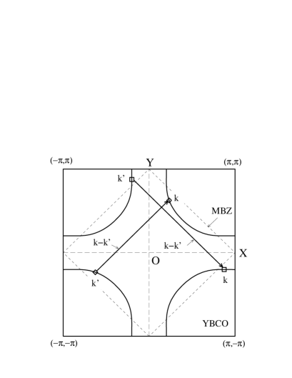
In the present study, the Stoner factor ${\alpha}_{\rm S}\equiv U\chi_{\bf Q}^{0}(0)$ at $T=0.02$ exceeds 0.99 both for $n=0.9$ (LSCO, YBCO) and $n=1.15$ (NCCO). (Note that ${\alpha}_{\rm S}<1$ at finite temperatures in two dimensional systems because Marmin-Wagner theorem is satisfied in the FLEX approximation.) In this case, $\chi_{\bf Q}^{s}\gg\chi_{\bf Q}^{c}$ is realized, and $V^{\rm FLEX}\approx(3U^{2}/2)\chi^{\rm s}$. Then, by reflecting the strong ${{\bf q}}$-dependence of $\chi_{{\bf q}}^{\rm s}$, $\gamma_{{\bf k}}\equiv{\rm Im}\Sigma_{{\bf k}}(-i\delta)$ on the FS becomes very anisotropic. ($\gamma_{{\bf k}}$ represents the quasiparticle damping rate.) $\gamma_{{\bf k}}$ takes a large value around the crossing points with the magnetic Brillouin zone (MBZ)-boundary, which we call hot spots as often referred to in literatures Rice ; Pines-Hall . On the other hand, $\gamma_{{\bf k}}$ takes the minimum value at the points where the distance from the MBZ-boundary is the largest, which are called cold spots. (see Fig. 1.) Transport phenomena for lower frequencies are governed by the electronic properties around the cold spot.

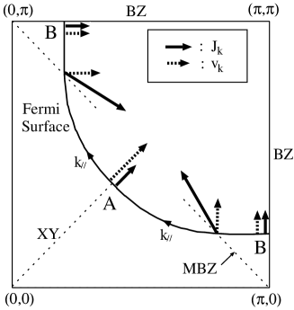
As shown in fig.1 (a), the location of the cold spot for hole-doped systems is around A. Whereas the cold spot for electron-doped systems locates around B: This fact was first predicted by ref. Kontani-Hall theoretically based on the FLEX approximation, and it is verified by the ARPES measurement later Armitage ; Armitage2 . The difference of the position of the cold spot explains the remarkable difference in transport phenomena between hole-doped systems and electron-doped ones Kontani-Hall . For example, both $R_{\rm H}$ and $S$ are positive in YBCO and LSCO whereas they are negative in NCCO.

In the present FLEX calculation for LSCO ($n=0.90$), the maximum (minimum) value of $\gamma_{{\bf k}}$ on the FS is 0.38 (0.12) at $T=0.02$. The ratio of anisotropy is 3.2, which is consistent with ARPES measurements in slightly under-doped compounds. Such a small anisotropy cannot account for the enhancement of $R_{\rm H}$ in under-doped systems within the RTA Pines-Hall . In the presence of strong AF fluctuations, however, the total current ${\bf J}_{{\bf k}}$ becomes quite different from the quasiparticle velocity ${\bf v}_{{\bf k}}$ due to the back-flow, which is totally dropped in the RTA Kontani-Hall . In fact, various anomalous transport phenomena in HTSC’s are brought by the nontrivial momentum-dependence of ${\bf J}_{{\bf k}}$ around the cold spot.

Finally, we discuss the dynamical spin susceptibility given by the FLEX approximation. Its phenomenological form is expressed as

$$\chi_{{\bf k}}^{\rm s}({\omega}+i\delta)\approx\frac{\chi_{Q}}{1+\xi^{2}({{\bf q}}-{{\bf Q}})^{2}-i{\omega}/{\omega}_{\rm sf}},$$ (9)

where $\xi$ is the AF correlation length, and ${{\bf Q}}$ is the nesting vector. ${{\bf Q}}=(\pi,\pi)$ in both YBCO and NCCO Kontani-Hall . $\chi_{Q}\propto 1/{\omega}_{\rm sf}\propto\xi^{2}$, and $\xi^{2}\propto T^{-1}$ in the FLEX approximation, which is equivalent to the SCR theory Moriya . Here we call eq.(9) the AF-fluctuation model.

II.2 Conserving approximation for ${\sigma}_{\mu\nu}({\omega})$

Here, we explain how to calculate the optical conductivity based on the Kubo formula. To satisfy the conservation laws, we have to take the current vertex correction (CVC) into account in accordance with the Ward identity.

According to the Kubo formula, the optical conductivity ${\sigma}_{xx}({\omega})\equiv{\sigma}({\omega})$ and the optical Hall conductivity ${\sigma}_{xy}({\omega})$ are given by

$${\sigma}_{\mu\nu}({\omega})=\frac{1}{i{\omega}}\left[K_{\mu\nu}^{\rm R}({\omega})-K_{\mu\nu}^{\rm R}(0)\right],$$ (10)

where $K_{\mu\nu}^{\rm R}({\omega})$ is the retarded current-current correlation function, which are given by the analytic continuations of the following thermal Green functions Eliashberg ; Kohno :

$$K_{xx}(i{\omega}_{l}) = -2e^{2}T\sum_{n,{{\bf k}}}v_{{{\bf k}}x}^{0}g_{{\bf k}}({\epsilon}_{n};{\omega}_{l})\Lambda_{{{\bf k}}x}({\epsilon}_{n};{\omega}_{l}),$$ (11)

$$K_{xy}(i{\omega}_{l}) = i\cdot 2e^{3}T\sum_{n,{{\bf k}}}\Lambda_{{{\bf k}}x}({\epsilon}_{n};{\omega}_{l})g_{{\bf k}}({\epsilon}_{n};{\omega}_{l})$$ (12)

$$\times\frac{1}{2}\left\{[G_{{\bf k}}({\epsilon}_{n}+{\omega}_{l})v_{{{\bf k}}x}({\epsilon}_{n}+{\omega}_{l})-G_{{\bf k}}({\epsilon}_{n})v_{{{\bf k}}x}({\epsilon}_{n})]\frac{{\partial}}{{\partial}k_{y}}-\langle x\leftrightarrow y\rangle\right\}\Lambda_{{{\bf k}}y}({\epsilon}_{n};{\omega}_{l}),$$

where $-e(e>0)$ represents the charge of an electron. Here we put $\hbar=c=1$. $g_{{\bf k}}({\epsilon}_{n};{\omega}_{l})\equiv G_{{\bf k}}({\epsilon}_{n}+{\omega}_{l})G_{{\bf k}}({\epsilon}_{n})$, $v_{{{\bf k}}\mu}^{0}\equiv{\partial}{\epsilon}_{{\bf k}}/{\partial}k_{\mu}$ is the velocity of the non-interacting electron with ${{\bf k}}$, and $\Lambda_{{{\bf k}}\mu}({\epsilon}_{n};{\omega}_{l})$ is the dressed current which is given by

$${\bf\Lambda}_{{{\bf k}}}({\epsilon}_{n};{\omega}_{l}) = {\bf v}_{{{\bf k}}}^{0}+T\sum_{m,{{\bf p}}}\Gamma_{{{\bf k}},{{\bf p}}}({\epsilon}_{n},{\epsilon}_{m};{\omega}_{l})g_{{\bf p}}({\epsilon}_{m};{\omega}_{l}){\bf v}_{{{\bf p}}}^{0}$$ (13)

$$= {\bf v}_{{{\bf k}}}^{0}+T\sum_{m,{{\bf p}}}\Gamma_{{{\bf k}},{{\bf p}}}^{\rm I}({\epsilon}_{n},{\epsilon}_{m};{\omega}_{l})g_{{\bf p}}({\epsilon}_{m};{\omega}_{l})$$

$$\times{\bf\Lambda}_{{{\bf p}}}({\epsilon}_{m};{\omega}_{l}),$$

where $\Gamma_{{{\bf k}},{{\bf p}}}({\epsilon}_{n},{\epsilon}_{m};{\omega}_{l})$ is the full four-point vertex function, and $\Gamma_{{{\bf k}},{{\bf p}}}^{\rm I}$ is the irreducible four-point vertex with respect to the particle-hole channel.

Equation (11) was derived by Eliashberg in 1962 Eliashberg . Equation (12) was first derived within the Born approximation Fukuyama . later it was proved to be exact for any Fermi liquid system up to the order of $O(\gamma^{-2})$, which is the most divergent term with respect to $\gamma^{-1}$ Kohno . In the same way, the general formulae for the magnetoresistance Kontani-MR-form , the thermoelectric power and the Nernst coefficient Kontani-S-form have been derived from the linear-response theory (Kubo formula) on the basis of the microscopic Fermi liquid theory.

In the numerical study of transport coefficients, one have to take account of the irreducible four point vertex $\Gamma^{\rm I}$ to satisfy the conservation laws, which is given by $\delta\Sigma^{\rm FLEX}/\delta G$ Baym-Kadanoff . In the FLEX approximation, $\Gamma^{\rm I}$ is expressed as

$$\Gamma_{{{\bf k}},{{\bf k}}^{\prime}}^{\rm I}({\epsilon}_{n},{\epsilon}_{n^{\prime}};{\omega}_{l}) = V_{{{\bf k}}-{{\bf k}}^{\prime}}^{\rm FLEX}({\epsilon}_{n}-{\epsilon}_{n^{\prime}})$$ (14)

$$-T\sum_{{{\bf p}}m}\left(G(k+k^{\prime}+p)+G(k-p)\right)G(-p+k^{\prime})W(p;p+{\omega}_{l}),$$

$$W(p;p+{\omega}_{l}) = \frac{3}{2}U^{2}(1+U\chi^{\rm s}(p))(1+U\chi^{\rm s}(p+{\omega}_{l}))+\frac{1}{2}U^{2}(1-U\chi^{\rm c}(p))(1+U\chi^{\rm c}(p+{\omega}_{l}))-U^{2},$$ (15)

where $k,k^{\prime},p=({{\bf k}},{\epsilon}_{n}),({{\bf k}}^{\prime},{\epsilon}_{n^{\prime}}),({{\bf p}},{\omega}_{l})$. In the light hand side of eq.(14), the first and the second terms are called the Maki-Thompson (MT) and the Aslamazov-Larkin (AL) terms, respectively, in literature.

Using the Green function given by the FLEX approximation, we numerically solve the Bethe-Salpeter equation for ${\bf\Lambda}$, eq.(13), by iteration. The kernel function $\Gamma^{\rm I}$ is given in eq.(14). Then, we obtain $K_{\mu\nu}(i{\omega}_{l})$ by inserting the obtained ${\bf\Lambda}$ into eqs.(11) and (12). The retarded function $K_{\mu\nu}^{\rm R}({\omega})$ is derived from the analytic continuation of $K_{\mu\nu}(i{\omega}_{l})$ with ${\omega}_{l}\geq 0$, using the numerical Pade approximation.

Pade approximation is less reliable when the function under consideration is strongly ${\omega}$-dependent, and when the temperature is high because the Matsubara frequency is sparse. To increase the accuracy of the Pade approximation, both $\Sigma({\epsilon}_{n})$ and ${\bf\Lambda}({\epsilon}_{n};{\epsilon}_{l})$ have to be obtained with high accuracy; their relative errors should be $10^{-8}\sim 10^{-10}$. In performing the Pade approximation, we utilize the fact that the $i{\omega}$-linear term of $K_{\mu\nu}({\omega})$ is equal to the DC value of ${\sigma}_{\mu\nu}$, which can be obtained within the FLEX approximation with high accuracy, as performed in refs. Kontani-review ; Kontani-MR ; Kontani-Hall ; Kontani-S ; Kontani-N . By imposing this constraint on the Pade approximation, we succeed in deriving the ${\sigma}_{\mu\nu}({\omega})$ with enough accuracy in the present study.

In the present numerical study, we take the infinite series of the MT-terms in ${\bf\Lambda}$, whereas we drop all the AL-terms in eq.(14). This simplification is justified for DC-conductivities when the AF fluctuations for ${\bf Q}\approx(\pi,\pi)$ are dominant, as proved in ref.Kontani-Hall . In the same way, AL-terms would be also negligible for IR optical conductivities. In fact, we have checked that the $f$-sum rule both for ${\sigma}({\omega})$ and ${\sigma}_{xy}({\omega})$ are well satisfied even if all the AL-terms are dropped, as will be shown in Fig.10. This results ensure the reliability of the present numerical study. (Although we have also tried to include the AL-terms, then the accuracy of the numerical Pade approximation became worse, unfortunately.)

In a Fermi liquid, the relaxation time $\tau_{{\bf k}}$ in the relaxation time approximation (RTA) is $1/2\gamma_{{\bf k}}\equiv 1/2{\rm Im}\Sigma_{{\bf k}}(-i\delta)$. Transport coefficients can be expanded in terms of $\gamma^{-1}$, which diverges as the temperature approaches zero. Equation (11) is formally an exact expression. On the other hand, eq.(12) gives an exact expression for ${\sigma}_{xy}({\omega})$ up to the order of $O(\gamma^{-2})$, which is the most divergent term with respect to $\gamma^{-1}$. Less singular terms, which are given as C and D in ref.Kohno (p.636) or the last two terms in Fig. 3 of ref.Kontani-S-form , are dropped in $K_{xy}$ given by eq.(12). In terms of the FLEX approximation, eq.(12) is exact beyond $O(\gamma^{-2})$ because both C and D vanish within this approximation Kontani-RH-kappa .

III ${\omega}$-linear term of ${\sigma}_{\mu\nu}({\omega})$: The role of the CVC

Based on the Kubo formula, we derive the general formula for the ${\omega}$-linear term of ${\sigma}_{\mu\nu}({\omega})$, which we denote $\Delta{\sigma}_{\mu\nu}$ hereafter. The relation ${\sigma}_{\mu\nu}({\omega})=\{{\sigma}_{\mu\nu}(-{\omega})\}^{\ast}$ tells that $\Delta{\sigma}_{\mu\nu}$ is pure imaginary. The most divergent terms of $\Delta{\sigma}\equiv\Delta{\sigma}_{xx}$ and $\Delta{\sigma}_{xy}$ are order of $O(\gamma^{-2})$ and $O(\gamma^{-3})$, respectively. The derived expressions in this section are exact up to the most divergent terms. Based on the derived expression, we discuss the role of the current vertex correction (CVC) for $\Delta{\sigma}_{xy}$, and find that it is strongly enhanced when the AF fluctuations ate strong. Readers who are not interested in the microscopic derivation can skip to the next section, where we will show the numerical results for ${\sigma}_{\mu\nu}({\omega})$ given by the CVC-FLEX approximation.

III.1 Exact expression for the ${\omega}$-linear term of ${\sigma}_{\mu\nu}({\omega})$

Here, we perform the analytic continuations of eq.(11) and (12) according to refs.Eliashberg and Kohno , and derive the general formula for $\Delta{\sigma}_{\mu\nu}({\omega})$. In preparation for analyzing the CVC in later sections, we derive the expressions without CVC, which corresponds to the relaxation time approximation (RTA) with ${{\bf k}}$- and ${\epsilon}$-dependent relaxation time $\tau_{{\bf k}}({\epsilon})$. After the analytic continuation of eq.(11),

$${\sigma}^{0}({\omega}) = e^{2}\sum_{{\bf k}}\int\frac{d{\epsilon}}{\pi}\frac{1}{2{\omega}}\left[{\rm th}\frac{{\epsilon}_{+}}{2T}-{\rm th}\frac{{\epsilon}_{-}}{2T}\right]$$ (16)

$$\times G_{{\bf k}}^{\rm R}({\epsilon}_{+})G_{{\bf k}}^{\rm A}({\epsilon}_{-})\{v_{{{\bf k}}x}^{0}\}^{2},$$

where ${\epsilon}_{\pm}\equiv{\epsilon}\pm{\omega}/2$, and we have dropped the terms with $G^{\rm R}({\epsilon}_{+})G^{\rm R}({\epsilon}_{-})$ and $G^{\rm A}({\epsilon}_{+})G^{\rm A}({\epsilon}_{-})$ because they are less divergent with respect to $\gamma^{-1}$, and they vanish at $T=0$ Eliashberg . Here we expand eq.(16) with respect to ${\omega}$:

$${\rm th}\frac{{\epsilon}_{+}}{2T}-{\rm th}\frac{{\epsilon}_{-}}{2T}=2{\omega}\left(-\frac{{\partial}f}{{\partial}{\epsilon}}\right)+O({\omega}^{2}),$$ (17)

$$G_{{\bf k}}^{\rm R}({\epsilon}_{+})G_{{\bf k}}^{\rm A}({\epsilon}_{-})=|G_{{\bf k}}({\epsilon})|^{2}+iz_{{\bf k}}^{-1}({\epsilon}){\omega}$$ (18)

$$\ \ \ \ \ \ \ \ \ \ \ \ \ \ \ \ \ \ \ \ \ \ \times|G_{{\bf k}}({\epsilon})|^{2}|{\rm Im}G_{{\bf k}}({\epsilon})|+O({\omega}^{2}),$$

where $z_{{\bf k}}({\epsilon})=(1-\frac{{\partial}}{{\partial}{\epsilon}}{\rm Re}\Sigma_{{\bf k}}({\epsilon}))^{-1}$ is the renormalization factor. At sufficiently lower temperature, the Green function for ${\omega}\sim 0$ and ${\epsilon}_{{\bf k}}\sim\mu$ is well approximated as

$$G_{{\bf k}}^{\rm R}({\omega})=\frac{z_{{\bf k}}}{{\omega}-{\epsilon}_{{\bf k}}^{\ast}+i\gamma_{{\bf k}}^{\ast}},$$ (19)

where ${\epsilon}_{{\bf k}}^{\ast}=z_{{\bf k}}({\epsilon}_{{\bf k}}+{\rm Re}\Sigma_{{\bf k}}(0)-\mu)$ and $\gamma_{{\bf k}}^{\ast}=z_{{\bf k}}\gamma_{{\bf k}}$. Equation is called the quasiparticle representation of Green function, whose validity is assured by the microscopic Fermi liquid theory. When eq.(19) is valid,

$$|{\rm Im}G_{{\bf k}}({\omega})|=\pi z_{{\bf k}}\delta({\omega}-{\epsilon}_{{\bf k}}^{\ast}),$$

$$|G_{{\bf k}}({\omega})|^{2}=\frac{\pi}{\gamma_{{\bf k}}}z_{{\bf k}}\delta({\omega}-{\epsilon}_{{\bf k}}^{\ast}),$$

$$|G_{{\bf k}}({\omega})|^{2}|{\rm Im}G_{{\bf k}}({\epsilon})|=\frac{\pi}{2\gamma_{{\bf k}}^{2}}z_{{\bf k}}\delta({\omega}-{\epsilon}_{{\bf k}}^{\ast}),$$ (20)

$$|G_{{\bf k}}({\omega})|^{4}=\frac{\pi}{2\gamma_{{\bf k}}^{3}}z_{{\bf k}}\delta({\omega}-{\epsilon}_{{\bf k}}^{\ast}),$$

$$|G_{{\bf k}}({\omega})|^{2}{\rm Re}G_{{\bf k}}^{2}({\epsilon})=-\frac{\pi}{4\gamma_{{\bf k}}^{3}}z_{{\bf k}}\delta({\omega}-{\epsilon}_{{\bf k}}^{\ast}),$$

for ${\omega},{\epsilon}_{{\bf k}}^{\ast}\sim 0$. As a result, the expression for ${\sigma}^{0}({\omega})$ expanded with respect to ${\omega}$ is

$${\sigma}^{0}({\omega}) = e^{2}\sum_{{\bf k}}\left(-\frac{{\partial}f}{{\partial}{\epsilon}}\right)\frac{\{v_{{{\bf k}}x}^{0}\}^{2}}{\gamma_{{\bf k}}}$$

$$+i{\omega}\cdot e^{2}\sum_{{\bf k}}\left(-\frac{{\partial}f}{{\partial}{\epsilon}}\right)\frac{z_{{\bf k}}^{-1}\{v_{{{\bf k}}x}^{0}\}^{2}}{2\gamma_{{\bf k}}^{2}}+O({\omega}^{2}).$$

In a free-dispersion model ${\epsilon}_{{\bf k}}=k^{2}/2m$, eq.(III.1) becomes

$${\sigma}^{0}({\omega}) = \frac{e^{2}n}{m\cdot 2\gamma}+iz^{-1}{\omega}\frac{e^{2}n}{m\cdot(2\gamma)^{2}}$$ (22)

$$\approx \frac{e^{2}n}{m(2\gamma-iz^{-1}{\omega})},$$

which is equal to the Drude form for ${\sigma}({\omega})$ given by the RTA if we replace $2\gamma$ with $\tau^{-1}$.

In the same way, ${\sigma}_{xy}({\omega})$ without CVC is given by the analytic continuation of eq.(12):

$${\sigma}_{xy}^{0}({\omega}) = -e^{3}\sum_{{\bf k}}\int\frac{d{\epsilon}}{\pi}\frac{1}{2{\omega}}[{\rm th}\frac{{\epsilon}_{+}}{2T}-{\rm th}\frac{{\epsilon}_{-}}{2T}]G_{{\bf k}}^{\rm R}({\epsilon}_{+})G_{{\bf k}}^{\rm A}({\epsilon}_{-})$$ (23)

$$\times\left[G_{{\bf k}}^{\rm R}({\epsilon}_{+})-G_{{\bf k}}^{\rm A}({\epsilon}_{-})\right]\frac{i}{2}A_{{{\bf k}}},$$

$$A_{{{\bf k}}} = v_{{{\bf k}}x}^{0}\left(v_{{{\bf k}}x}^{0}\frac{{\partial}}{{\partial}k_{y}}-v_{{{\bf k}}y}^{0}\frac{{\partial}}{{\partial}k_{x}}\right)v_{{{\bf k}}y}^{0},$$ (24)

where we have dropped CVC for the quasiparticle velocity given by the momentum derivative of the self-energy. Up to the order of $O({\omega})$, we see that

$$G_{{\bf k}}^{\rm R}G_{{\bf k}}^{\rm A}\left[G_{{\bf k}}^{\rm R}-G_{{\bf k}}^{\rm A}\right]\frac{i}{2}=|G_{{\bf k}}({\epsilon})|^{2}|{\rm Im}G_{{\bf k}}({\epsilon})|$$

$$\ \ \ \ \ \ \ \ \ \ \ \ \ \ \ +iz_{{\bf k}}^{-1}{\omega}\left\{\frac{1}{2}|G_{{\bf k}}({\epsilon})|^{4}-|G_{{\bf k}}({\epsilon})|^{2}{\rm Re}G_{{\bf k}}^{2}({\epsilon})\right\}$$

$$\ \ \ \ \ \ \ \ \ \ \ \ \ \approx\frac{\pi}{2\gamma_{{\bf k}}^{2}}z_{{\bf k}}^{-1}\delta({\epsilon}-{\epsilon}_{{\bf k}}^{\ast})+iz_{{\bf k}}^{-1}{\omega}\frac{\pi}{2\gamma_{{\bf k}}^{3}}\delta({\epsilon}-{\epsilon}_{{\bf k}}^{\ast}).$$

As a result, the expression for ${\sigma}_{xy}^{0}({\omega})$ within the order of $O({\omega})$ is

$${\sigma}_{xy}^{0}({\omega}) = -e^{3}\sum_{{\bf k}}\left(-\frac{{\partial}f}{{\partial}{\epsilon}}\right)\frac{A_{{\bf k}}}{2\gamma_{{\bf k}}^{2}}$$ (26)

$$+i{\omega}\cdot(-e^{3})\sum_{{\bf k}}\left(-\frac{{\partial}f}{{\partial}{\epsilon}}\right)\frac{z_{{\bf k}}^{-1}A_{{\bf k}}}{2\gamma_{{\bf k}}^{3}}.$$

In a free-dispersion model, eq.(26) becomes

$${\sigma}_{xy}^{0}({\omega}) = \frac{-e^{3}n}{m^{2}\cdot(2\gamma)^{2}}+2iz^{-1}{\omega}\frac{-e^{3}n}{m^{2}\cdot(2\gamma)^{3}}$$ (27)

$$\approx \frac{-e^{3}n}{m^{2}(2\gamma-iz^{-1}{\omega})^{2}},$$

which is also equal to the Drude formula given by the RTA.

In the next stage, we derive the general expression for $\Delta{\sigma}_{\mu\nu}$ by taking all the CVC’s into account. After the analytic continuations of eqs.(11) and (12) Eliashberg ; Kohno ,

$${\sigma}({\omega}) = e^{2}\sum_{{\bf k}}\int\frac{d{\epsilon}}{\pi}\left(-\frac{{\partial}f}{{\partial}{\epsilon}}\right){\tilde{v}}_{{{\bf k}}x}({\epsilon};{\omega})g_{{\bf k}}^{(2)}({\epsilon};{\omega})J_{{{\bf k}}x}({\epsilon};{\omega}),$$ (28)

$${\sigma}_{xy}({\omega}) = -e^{3}\sum_{{\bf k}}\int\frac{d{\epsilon}}{\pi}\left(-\frac{{\partial}f}{{\partial}{\epsilon}}\right)J_{{{\bf k}}x}({\epsilon};{\omega})g_{{\bf k}}^{(2)}({\epsilon};{\omega})$$ (29)

$$\times\frac{i}{2}\left[\left([G_{{\bf k}}^{\rm R}v_{{{\bf k}}x}^{\rm R}]_{{\epsilon}_{+}}-[G_{{\bf k}}^{\rm A}v_{{{\bf k}}x}^{\rm A}]_{{\epsilon}_{-}}\right)\frac{{\partial}}{{\partial}k_{y}}-\langle x\leftrightarrow y\rangle\right]J_{{{\bf k}}y}({\epsilon};{\omega}),$$

where $g_{{\bf k}}^{(1)}({\epsilon};{\omega})=G_{{\bf k}}^{\rm R}({\epsilon}_{+})G_{{\bf k}}^{\rm R}({\epsilon}_{-})$, $g_{{\bf k}}^{(2)}({\epsilon};{\omega})=G_{{\bf k}}^{\rm R}({\epsilon}_{+})G_{{\bf k}}^{\rm A}({\epsilon}_{-})$ and $g_{{\bf k}}^{(3)}({\epsilon};{\omega})=G_{{\bf k}}^{\rm A}({\epsilon}_{+})G_{{\bf k}}^{\rm A}({\epsilon}_{-})$. $v_{{{\bf k}}\mu}^{\rm R}({\epsilon})=v_{{{\bf k}}\mu}^{0}+\frac{{\partial}}{{\partial}k_{\mu}}\Sigma_{{\bf k}}^{\rm R}({\epsilon})$. $G^{\rm R}$ and $G^{\rm A}$ are the retarded and advanced Green functions, respectively. ${\bf J}$, ${\bf v}$ and ${\bf\tilde{v}}$ are given by

$${\bf J}_{{{\bf k}}}({\epsilon};{\omega}) = {\bf v}_{{{\bf k}}}({\epsilon};{\omega})+\sum_{{{\bf q}}}\int\frac{d{\epsilon}^{\prime}}{4\pi i}{\cal T}_{22}({{\bf k}}{\epsilon},{{\bf q}}{\epsilon}^{\prime};{\omega})g_{{{\bf q}}}^{(2)}({\epsilon}^{\prime};{\omega}){\bf v}_{{{\bf k}}}({\epsilon}^{\prime};{\omega})$$ (30)

$$= {\bf v}_{{{\bf k}}}({\epsilon};{\omega})+\sum_{{{\bf q}}}\int\frac{d{\epsilon}^{\prime}}{4\pi i}{\cal T}_{22}^{(0)}({{\bf k}}{\epsilon},{{\bf q}}{\epsilon}^{\prime};{\omega})g_{{{\bf q}}}^{(2)}({\epsilon}^{\prime};{\omega}){\bf J}_{{{\bf k}}}({\epsilon}^{\prime};{\omega}),$$

$${\bf v}_{{{\bf k}}}({\epsilon};{\omega}) = {\bf v}_{{{\bf k}}}^{0}+\sum_{{{\bf q}},j=1,3}\int\frac{d{\epsilon}^{\prime}}{4\pi i}{\cal T}_{2j}^{(0)}({{\bf k}}{\epsilon},{{\bf q}}{\epsilon}^{\prime};{\omega})g_{{{\bf q}}}^{(j)}({\epsilon}^{\prime};{\omega}){\bf v}_{{{\bf q}}}^{0},$$ (31)

$${\bf\tilde{v}}_{{{\bf k}}}({\epsilon};{\omega}) = {\bf v}_{{{\bf k}}}^{0}+\sum_{{{\bf q}},j=1,3}(j-2)\int\frac{d{\epsilon}^{\prime}}{4\pi i}{\bf v}_{{{\bf q}}}^{0}\cdot{\rm th}\left(\frac{{\epsilon}^{\prime}+(j-2){\omega}/2}{2T}\right)g_{{{\bf q}}}^{(j)}({\epsilon}^{\prime};{\omega})\Gamma_{j2}({{\bf q}}{\epsilon}^{\prime},{{\bf k}}{\epsilon};{\omega}),$$ (32)

where the definition of ${\cal T}_{22}^{(0)}({{\bf k}}{\epsilon},{{\bf q}}{\epsilon}^{\prime};{\omega})$ is given in ref.Eliashberg . ${\cal T}_{22}^{(0)}$ is a subgroup of ${\cal T}_{22}$ which is irreducible with respect to $g_{{{\bf q}}}^{(2)}$, whereas it is reducible with respect to $g_{{{\bf q}}}^{(1,3)}$. The following Bethe-Salpeter equation holds; ${\cal T}_{22}={\cal T}_{22}^{(0)}+\sum\int{\cal T}_{22}^{(0)}g^{(2)}{\cal T}_{22}$.

As explained in ref.Eliashberg , ${v}_{{{\bf k}}x}({\epsilon};{\omega}=0)={\tilde{v}}_{{{\bf k}}x}({\epsilon};{\omega}=0)={\rm Re}v_{{\bf k}}^{\rm R}({\epsilon})\equiv v_{{\bf k}}({\epsilon})$ is well satisfied in a Fermi liquid. As a result Eliashberg ; Kohno ,

$${\sigma}(0) = e^{2}\sum_{{\bf k}}\int\frac{d{\epsilon}}{\pi}\left(-\frac{{\partial}f}{{\partial}{\epsilon}}\right)|G_{{\bf k}}({\epsilon})|^{2}{v}_{{{\bf k}}x}({\epsilon})J_{{{\bf k}}x}({\epsilon}),$$ (33)

$${\sigma}_{xy}(0) = -e^{3}\sum_{{\bf k}}\int\frac{d{\epsilon}}{\pi}\left(-\frac{{\partial}f}{{\partial}{\epsilon}}\right)|G_{{\bf k}}({\epsilon})|^{2}|{\rm Im}G_{{\bf k}}({\epsilon})||{\bf v}_{{{\bf k}}}({\epsilon})|{J}_{{{\bf k}}x}({\epsilon})\frac{{\partial}}{{\partial}k_{\parallel}}J_{{{\bf k}}y}({\epsilon})$$ (34)

$$= -e^{3}\sum_{{\bf k}}\int\frac{d{\epsilon}}{2\pi}\left(-\frac{{\partial}f}{{\partial}{\epsilon}}\right)|G_{{\bf k}}({\epsilon})|^{2}|{\rm Im}G_{{\bf k}}({\epsilon})||{\bf v}_{{{\bf k}}}({\epsilon})|\left({\bf J}_{{{\bf k}}}({\epsilon})\times\frac{{\partial}{\bf J}_{{{\bf k}}}({\epsilon})}{{\partial}k_{\parallel}}\right)_{z},$$

where $k_{\parallel}\equiv({\hat{e}}_{z}\times{\bf v})/|{\bf v}|$, which is parallel to the Fermi surface. In deriving the first line in eq.(34), we have used the relation $v_{{{\bf k}}x}\frac{{\partial}}{{\partial}k_{y}}-v_{{{\bf k}}y}\frac{{\partial}}{{\partial}k_{x}}=({\hat{e}}_{z}\times{\bf v})\nabla=|{\bf v}|\frac{{\partial}}{{\partial}k_{\parallel}}$. The Onsager’s relation ${\sigma}_{xy}=-{\sigma}_{yx}$ is used in deriving the second line in eq.(34).

Here we expand ${\bf J}_{{{\bf k}}}({\epsilon};{\omega})$ with respect to ${\omega}$ as ${\bf J}_{{{\bf k}}}({\epsilon}=0;{\omega})={\bf J}_{{{\bf k}}}(0)+i{\omega}{\bf J}_{{{\bf k}}}^{(1)}(0)$. From eq.(30), one can check that the most divergent term of ${\bf J}_{{{\bf k}}}^{(1)}$ is proportional to $\gamma^{-1}$, which comes from the ${\omega}$-derivative of $g^{(2)}$ or that of the thermal factor in ${\cal T}_{22}^{(0)}$; $\frac{{\partial}}{{\partial}{\omega}}{\cal T}_{22}^{(0)}({\epsilon},{\epsilon}^{\prime};{\omega})\approx 2(-{\partial}f/{\partial}{\epsilon}^{\prime}){\rm Re}\Gamma(0,0)+O({\omega}^{2})$. For simplicity, we denote hereafter $J({\epsilon};{\omega}=0)\equiv J({\epsilon})$, $\Gamma({{\bf k}}{\epsilon},{{\bf p}}{\epsilon}^{\prime};{\omega}=0)\equiv\Gamma({{\bf k}}{\epsilon},{{\bf p}}{\epsilon}^{\prime})$, and so on. On the other hand, the ${\omega}$-linear term of eq.(31) or (32) is not singular with respect to $\gamma^{-1}$, so we put ${\omega}=0$ in eqs.(31) and (32) hereafter.

Using the relations in eq.(20), ${\bf J}_{{{\bf k}}}^{(1)}\propto\gamma^{-1}$ is given by

$${\bf J}_{{{\bf k}}}^{(1)} = \sum_{{{\bf q}}}\frac{1}{4i}{\cal T}_{22}({{\bf k}}0,{{\bf q}}{\epsilon}_{{{\bf q}}}^{\ast})\frac{z_{{\bf q}}}{\gamma_{{{\bf q}}}}\cdot\frac{{\bf J}_{{{\bf q}}}}{2\gamma_{{{\bf q}}}^{\ast}}$$ (35)

$$-\sum_{{{\bf q}}}\frac{1}{4i}\left(4i\delta_{{{\bf k}},{{\bf q}}}+{\cal T}_{22}({{\bf k}}0,{{\bf q}}{\epsilon}_{{{\bf q}}}^{\ast})\frac{z_{{{\bf q}}}}{\gamma_{{{\bf q}}}}\right)$$

$$\times\sum_{{{\bf q}}^{\prime}}{\rm Re}\Gamma({{\bf q}},{{\bf q}}^{\prime})\left(-\frac{{\partial}f}{{\partial}{\epsilon}}\right)_{{\epsilon}_{{{\bf q}}^{\prime}}^{\ast}}z_{{{\bf q}}^{\prime}}\frac{{\bf J}_{{{\bf q}}^{\prime}}}{2\gamma_{{{\bf q}}^{\prime}}}$$

$$\equiv {\bf L}_{{{\bf k}}}+{\bf M}_{{{\bf k}}},$$

where the first and the second terms come from the ${\omega}$-derivatives of $g^{(2)}$ and ${\cal T}_{22}^{(0)}$, respectively. Then, the ${\omega}$-linear term of the conductivity, which we denote as $\Delta{\sigma}_{\mu\nu}$, is given by

$$\Delta{\sigma} = i{\omega}\cdot e^{2}\sum_{{\bf k}}\left(-\frac{{\partial}f}{{\partial}{\epsilon}}\right)\left[\frac{z_{{\bf k}}^{-1}v_{{{\bf k}}x}J_{{{\bf k}}x}}{2\gamma_{{\bf k}}^{2}}+\frac{v_{{{\bf k}}x}J_{{{\bf k}}x}^{(1)}}{\gamma_{{\bf k}}}\right],$$

$$\Delta{\sigma}_{xy} = i{\omega}\cdot(-e^{3})\sum_{{\bf k}}\left(-\frac{{\partial}f}{{\partial}{\epsilon}}\right)\left[\frac{z_{{\bf k}}^{-1}A_{{\bf k}}}{2\gamma_{{\bf k}}^{3}}+\frac{B_{{\bf k}}}{2\gamma_{{\bf k}}^{2}}\right],$$ (37)

$$A_{{\bf k}} = J_{{{\bf k}}x}|{\bf v}_{{\bf k}}|\frac{{\partial}}{{\partial}k_{\parallel}}J_{{{\bf k}}y},$$ (38)

$$B_{{\bf k}} = J_{{{\bf k}}x}^{(1)}|{\bf v}_{{\bf k}}|\frac{{\partial}}{{\partial}k_{\parallel}}J_{{{\bf k}}y}+J_{{{\bf k}}x}|{\bf v}_{{\bf k}}|\frac{{\partial}}{{\partial}k_{\parallel}}J_{{{\bf k}}y}^{(1)},$$ (39)

where $|{\bf v}_{{\bf k}}|\frac{{\partial}}{{\partial}k_{\parallel}}=v_{{{\bf k}}x}\frac{{\partial}}{{\partial}k_{y}}-v_{{{\bf k}}y}\frac{{\partial}}{{\partial}k_{x}}$ as explained before. They are exact with respect to the most divergent terms with respect to $\gamma^{-1}$. Note that $\Delta{\sigma}_{\mu\nu}$ is pure imaginary.

Here, we further analyze ${\bf J}_{{\bf k}}^{(1)}$ given in eq. (35). First, ${\bf L}_{{{\bf k}}}$ is given by the following Bethe-Salpeter equation:

$${\bf P}_{{{\bf k}}} = \frac{{\bf J}_{{{\bf k}}}}{2\gamma_{{\bf k}}^{\ast}}+\sum_{{{\bf q}}}\frac{1}{4i}{\cal T}_{22}({{\bf k}}0,{{\bf q}}{\epsilon}_{{{\bf q}}}^{\ast})\frac{z_{{{\bf q}}}}{\gamma_{{{\bf q}}}}\cdot\frac{{\bf J}_{{{\bf q}}}}{2\gamma_{{{\bf q}}}^{\ast}}$$ (40)

$$= \frac{{\bf J}_{{{\bf k}}}}{2\gamma_{{\bf k}}^{\ast}}+\sum_{{{\bf q}}}\frac{1}{4i}{\cal T}_{22}^{\rm I}({{\bf k}}0,{{\bf q}}{\epsilon}_{{{\bf q}}}^{\ast})\frac{z_{{{\bf q}}}}{\gamma_{{{\bf q}}}}\cdot{\bf P}_{{{\bf q}}},$$

$${\bf L}_{{{\bf k}}} = {\bf P}_{{{\bf k}}}-\frac{{\bf J}_{{{\bf k}}}}{2\gamma_{{\bf k}}^{\ast}},$$ (41)

where ${\cal T}_{22}^{\rm I}({{\bf k}}0,{{\bf q}}{\epsilon}_{{{\bf q}}}^{\ast})=2i{\rm Im}V_{{{\bf k}}-{{\bf q}}}^{\rm R}({\epsilon}_{{{\bf q}}}^{\ast})({\rm cth}({\epsilon}_{{{\bf q}}}^{\ast}/2T)-{\rm th}({\epsilon}_{{{\bf q}}}^{\ast}/2T))$ in the FLEX approximation. In a similar way, ${\bf M}_{{{\bf k}}}$ is rewritten as

$${\bf M}_{{{\bf k}}} = {\bf N}_{{{\bf k}}}+\sum_{{{\bf q}}}\frac{1}{4i}{\cal T}_{22}^{\rm I}({{\bf k}}0,{{\bf q}}{\epsilon}_{{{\bf q}}}^{\ast})\frac{z_{{{\bf q}}}}{\gamma_{{{\bf q}}}}\cdot{\bf M}_{{{\bf q}}},$$ (42)

$${\bf N}_{{{\bf k}}} = -\sum_{{{\bf q}}}{\rm Re}\Gamma({{\bf k}},{{\bf q}})\left(-\frac{{\partial}f}{{\partial}{\epsilon}}\right)_{{\epsilon}_{{{\bf q}}}^{\ast}}z_{{{\bf q}}}\frac{{\bf J}_{{{\bf q}}}}{2\gamma_{{{\bf q}}}}.$$ (43)

At sufficiently lower temperatures, the expression for $\Delta{\sigma}_{\mu\nu}({\omega})$ in eq.(37) is rewritten by using ${\bf{\tilde{J}}}_{{{\bf k}}}^{(1)}$ (instead of ${\bf{J}}_{{{\bf k}}}^{(1)}$) as,

$$\Delta{\sigma} = i{\omega}\cdot e^{2}\sum_{{\bf k}}\left(-\frac{{\partial}f}{{\partial}{\epsilon}}\right)\frac{v_{{{\bf k}}x}{\tilde{J}}_{{\bf k}}^{(1)}}{\gamma_{{\bf k}}},$$ (44)

$$\Delta{\sigma}_{xy} = i{\omega}\cdot(-e^{3})\sum_{{\bf k}}\left(-\frac{{\partial}f}{{\partial}{\epsilon}}\right)\frac{z_{{\bf k}}^{-1}{\tilde{B}}_{{\bf k}}}{2\gamma_{{\bf k}}^{2}},$$ (45)

$${\tilde{B}}_{{\bf k}} = {\tilde{J}}_{{{\bf k}}x}^{(1)}|{\bf v}_{{\bf k}}|\frac{{\partial}}{{\partial}k_{\parallel}}J_{{{\bf k}}y}+J_{{{\bf k}}x}|{\bf v}_{{\bf k}}|\frac{{\partial}}{{\partial}k_{\parallel}}{\tilde{J}}_{{{\bf k}}y}^{(1)},$$ (46)

$${\bf\tilde{J}}_{{{\bf k}}}^{(1)} = {\bf P}_{{{\bf k}}}+{\bf M}_{{{\bf k}}}={\bf J}_{{{\bf k}}}^{(1)}+\frac{{\bf J}_{{{\bf k}}}}{2\gamma_{{\bf k}}^{\ast}}.$$ (47)

In the next subsection, we will discuss the temperature dependence of $\Delta{\sigma}_{xy}$ when the AF fluctuations are strong, by analyzing the ${{\bf k}}$-dependence of ${\bf\tilde{J}}_{{{\bf k}}}^{(1)}$. We will approximately solve the Bethe-Salpeter equations (40) and (42) based on the AF-fluctuation model.

In a Fermi liquid, $\gamma_{{\bf k}}$ and $z_{{\bf k}}$ are expressed as

$$\gamma_{{\bf k}} = \frac{1}{4i}\sum_{{{\bf q}}}\int d{\epsilon}{\cal T}_{22}^{\rm I}({{\bf k}}0,{{\bf q}}{\epsilon})\rho_{{{\bf q}}}({\epsilon})$$ (48)

$$\approx \frac{1}{4i}\sum_{{{\bf q}}}{\cal T}_{22}^{\rm I}({{\bf k}}0,{{\bf q}}{\epsilon}_{{{\bf q}}}^{\ast})z_{{{\bf q}}},$$

$$z_{{\bf k}}^{-1}-1 = -\left.\frac{{\partial}}{{\partial}{\epsilon}}{\rm Re}\Sigma_{{\bf k}}({\epsilon})\right|_{{\epsilon}=0}$$ (49)

$$= \sum_{{\bf q}}{\rm Re}\Gamma({{\bf k}},{{\bf q}})\left(-\frac{{\partial}f}{{\partial}{\epsilon}}\right)_{{\epsilon}_{{{\bf q}}}^{\ast}}z_{{{\bf q}}}$$

$$-\frac{{\partial}}{{\partial}\mu}{\rm Re}\Sigma_{{\bf k}}(0).$$

Note that the uniform charge susceptibility in a Fermi liquid is given by $\displaystyle\chi_{\rm c}=[1-{{\partial}}{\rm Re}\Sigma_{{\bf k}}(0)/{{\partial}\mu}]\chi_{\rm c}^{0}$, where $\chi_{\rm c}^{0}$ is the susceptibility for $U=0$. Because $\chi_{\rm c}\ll\chi_{\rm c}^{0}$ is expected in strongly correlated systems (like in heavy Fermion systems), the relation ${{\partial}}{\rm Re}\Sigma_{{\bf k}}(0)/{{\partial}\mu}\raisebox{-3.22916pt}[-6.45831pt]{$\;\stackrel{{\scriptstyle<}}{{\sim}}\;$}1$ should be satisfied. This relation is also expected to be realized in HTSC according to the FLEX approximation.

III.2 Role of the CVC in the presence of AF fluctuations

Using the general expression for $\Delta{\sigma}_{\mu\nu}$ derived in the previous subsection, we discuss its temperature dependence when the AF fluctuations are strong. For that purpose, we approximately analyze the CVC included in the expression for ${\sigma}_{\mu\nu}({\omega})$ based on the AF fluctuation model given in eq.(9).

First, we explain the total current for the DC-conductivity. The Bethe-Salpeter equation eq.(30) is rewritten at lower temperatures as Kontani-Hall

$${\bf J}_{{{\bf k}}}={\bf v}_{{{\bf k}}}+\sum_{{{\bf p}}}{\cal T}_{22}^{\rm I}({{\bf k}}0,{{\bf p}}{\epsilon}_{{\bf p}}^{\ast})z_{{{\bf p}}}\cdot\frac{1}{\gamma_{{\bf p}}}\cdot{\bf J}_{{{\bf p}}}$$ (50)

for ${\epsilon}={\omega}=0$. In the FLEX approximation, ${\cal T}_{22}({{\bf k}}0,{{\bf p}}{\epsilon})\approx 3U^{2}\cdot i{\rm Im}\chi_{{{\bf k}}-{{\bf p}}}^{\rm s}({\epsilon}+i\delta)[{\rm cth}({\epsilon}/2T)-{\rm th}({\epsilon}/2T)]$. Due to the thermal factor, ${\cal T}_{22}({{\bf k}}0,{{\bf p}}{\epsilon})$ takes large value only when $|{\epsilon}|\raisebox{-3.22916pt}[-6.45831pt]{$\;\stackrel{{\scriptstyle<}}{{\sim}}\;$}T$. If we apply the AF-fluctuation model, eq.(9), the main contributions of the ${{\bf p}}$-summation in eq.(50) come from the region $|{{\bf p}}-{{\bf k}}^{\prime}|\raisebox{-3.22916pt}[-6.45831pt]{$\;\stackrel{{\scriptstyle<}}{{\sim}}\;$}1/\xi$, where ${{\bf k}}^{\prime}$ is the momentum on the FS defined as $(k_{x}^{\prime},k_{y}^{\prime})=-{\rm sgn}(k_{x}k_{y})\cdot(k_{y},k_{x})$, as shown in Fig. 1 (b). We see the relation ${{\bf k}}-{{\bf k}}^{\prime}\approx{{\bf Q}}$ is satisfied on the FS. Here we assume $|{{\bf Q}}-({{\bf k}}-{{\bf k}}^{\prime})|\raisebox{-3.22916pt}[-6.45831pt]{$\;\stackrel{{\scriptstyle<}}{{\sim}}\;$}\xi^{-1}$ even at the cold spot, which is in fact satisfied in the present FLEX approximation for hole-doped systems Kontani-Hall . In this case, $\gamma_{{{\bf k}}_{\rm c}}\propto T$ is satisfied.

Taking account of the expression for $\gamma_{{\bf k}}$ given in eq.(48), we obtain a simplified Bethe-Salpeter equation Kontani-Hall ,

$${\bf J}_{{\bf k}}={\bf v}_{{\bf k}}+{\alpha}_{{\bf k}}\cdot{\bf J}_{{{\bf k}}^{\prime}}.$$ (51)

where ${\alpha}_{{\bf k}}=|\sum_{{{\bf p}}}{\cal T}_{22}^{\rm I}({{\bf k}}0,{{\bf p}}{\epsilon}_{{\bf p}}^{\ast})z_{{{\bf p}}}{\bf J}_{{{\bf p}}}/\gamma_{{\bf p}}|/|{\bf J}_{{{\bf k}}}|$. According to the AF-fluctuation model, ${\alpha}_{{\bf k}}\approx\langle\ \cos(\theta_{J}({{\bf q}})\!-\!\theta_{J}({{\bf k}}^{\prime}))\ \rangle_{|{{\bf q}}-{{\bf k}}^{\prime}|<1/\xi}\approx(1-c/\xi^{2})<1$ where $c\sim O(1)$ is a constant. ${\alpha}_{{\bf k}}$ takes the maximum value around hot spots. The solution of eq. (51) is Kontani-Hall

$${\bf J}_{{{\bf k}}}=\frac{1}{1-{\alpha}_{{\bf k}}^{2}}\left({\bf v}_{{{\bf k}}}+{\alpha}_{{\bf k}}\cdot{\bf v}_{{{\bf k}}^{\prime}}\right),$$ (52)

whose schematic behavior is shown in fig. 1 (b). Note that $(v_{{{\bf k}}^{\prime}x},v_{{{\bf k}}^{\prime}y})=-{\rm sgn}(k_{x}k_{y})\cdot(v_{{{\bf k}}y},v_{{{\bf k}}x})$ and $(J_{{{\bf k}}^{\prime}x},J_{{{\bf k}}^{\prime}y})=-{\rm sgn}(k_{x}k_{y})\cdot(J_{{{\bf k}}y},J_{{{\bf k}}x})$.

We stress that the same vertex functions ${\cal T}_{22}({{\bf k}}0,{{\bf p}}{\epsilon})$ appear in eqs.(30) and (48), which is the consequence of the Ward identity and is satisfied in any conserving approximation. This fact assures that the relation $1-{\alpha}\propto\xi^{2}$ holds even beyond the FLEX approximation.

In the same way, we study ${\bf{\tilde{J}}}_{{\bf k}}^{(1)}={\bf P}_{{\bf k}}+{\bf M}_{{\bf k}}$. The Bethe-Salpeter equation for ${\bf P}_{{\bf k}}$, eq. (40), is simplified as

$${\bf P}_{{{\bf k}}}\approx\frac{{\bf J}_{{{\bf k}}}}{2\gamma_{{\bf k}}^{\ast}}+{\alpha}_{{{\bf k}}}{\bf P}_{{{\bf k}}^{\prime}},$$ (53)

where ${\alpha}_{{{\bf k}}}$ is the same as that in eq.(51). The solution is given by

$${\bf P}_{{{\bf k}}}\approx\frac{1}{2\gamma_{{\bf k}}^{\ast}}\frac{{\bf J}_{{\bf k}}+{\alpha}_{{\bf k}}{\bf J}_{{{\bf k}}^{\prime}}}{1-{\alpha}_{{\bf k}}^{2}}.$$ (54)

Next, we analyze ${\bf N}_{{\bf k}}$ in eq.(43). Considering the relation ${\rm Re}\Gamma_{{{\bf k}},{{\bf q}}}\sim z^{-1}{\rm Re}V_{{{\bf k}}-{{\bf q}}}^{\rm FLEX}(0)$, we obtain

$${\bf N}_{{{\bf k}}} \approx -\frac{{\bf J}_{{{\bf k}}^{\prime}}}{2\gamma_{{{\bf k}}}}\cdot{\bar{\alpha}}_{{\bf k}}\sum_{{{\bf q}}}{\rm Re}\Gamma({{\bf k}},{{\bf q}})\left(-\frac{{\partial}f}{{\partial}{\epsilon}}\right)_{{\epsilon}_{{{\bf q}}}^{\ast}}z_{{{\bf q}}},$$ (55)

where ${\bar{\alpha}}_{{\bf k}}\raisebox{-3.22916pt}[-6.45831pt]{$\;\stackrel{{\scriptstyle<}}{{\sim}}\;$}{{\alpha}}_{{\bf k}}$ is expected in general because the momentum dependence of ${\rm Im}V_{{{\bf k}}-{{\bf p}}}^{\rm FLEX}({\epsilon})/{\epsilon}$ is much prominent than that of ${\rm Re}V_{{{\bf k}}-{{\bf p}}}^{\rm FLEX}(0)$, which are included in eqs.(50) and (55), respectively. Actually, ${\rm Im}\chi_{{\bf q}}^{\rm s}({\omega})/{\omega}\propto\{\chi_{{\bf q}}^{\rm s}(0)\}^{2}\propto\xi^{4}(1+\xi^{2}({\bf Q}-{{\bf q}})^{2})^{-2}$ according to eq. (9). In fact, in the present FLEX calculation for LSCO ($n=0.90$), the maximum (minimum) value of Im$\Sigma_{{\bf k}}(-i\delta)$ on the FS is 0.38 (0.12) at $T=0.02$; the ratio of anisotropy is 3.2, reflecting the sharp ${{\bf q}}$-dependence of ${\rm Im}\chi_{{\bf q}}^{\rm s}({\omega})/{\omega}$. On the other hand, the maximum (minimum) value of $z_{{\bf k}}^{-1}-1$ on the FS is 5.0 (3.8); the ratio of anisotropy is only 1.4.

Considering eq.(49), we rewrite eq.(55) as

$${\bf N}_{{{\bf k}}} \approx -\frac{{\bf J}_{{{\bf k}}^{\prime}}}{2\gamma_{{{\bf k}}}}\cdot{\bar{\alpha}}_{{\bf k}}\left(z_{{\bf k}}^{-1}-\chi_{\rm c}/\chi_{\rm c}^{0}\right)\equiv-{\tilde{\alpha}}_{{\bf k}}\frac{{\bf J}_{{{\bf k}}^{\prime}}}{2\gamma_{{{\bf k}}}^{\ast}}.$$ (56)

${\tilde{\alpha}}_{{\bf k}}\raisebox{-3.22916pt}[-6.45831pt]{$\;\stackrel{{\scriptstyle<}}{{\sim}}\;$}{\bar{\alpha}}_{{\bf k}}\raisebox{-3.22916pt}[-6.45831pt]{$\;\stackrel{{\scriptstyle<}}{{\sim}}\;$}{{\alpha}}_{{\bf k}}$ should be satisfied because $\chi_{\rm c}/\chi_{\rm c}^{0}$ is positive. We note again that $\chi_{\rm c}/\chi_{\rm c}^{0}\ll 1$ in strongly correlated systems. Then, the approximate solution of eq.(42) is

$${\bf M}_{{{\bf k}}}\approx-\frac{{\tilde{\alpha}}_{{\bf k}}}{2\gamma_{{\bf k}}^{\ast}}\frac{{\alpha}_{{\bf k}}{\bf J}_{{\bf k}}+{\bf J}_{{{\bf k}}^{\prime}}}{1-{\alpha}_{{\bf k}}^{2}}.$$ (57)

In conclusion, an approximate expression for ${\sigma}_{xy}({\omega})$ up to the order of $O({\omega})$ is given by

$${\sigma}_{xy}({\omega}) = -e^{3}\sum_{{\bf k}}\left(-\frac{{\partial}f}{{\partial}{\epsilon}}\right)|{\bf v}_{{\bf k}}|\frac{1}{4\gamma_{{\bf k}}^{2}}$$ (58)

$$\times\left({\bf\tilde{J}}_{{\bf k}}(0;{\omega})\times\frac{{\partial}{\bf\tilde{J}}_{{\bf k}}(0;{\omega})}{{\partial}k_{\parallel}}\right)_{z},$$

$${\bf\tilde{J}}_{{\bf k}}(0;{\omega}) = {\bf J}_{{\bf k}}(0;{\omega})+i{\omega}\frac{{\bf J}_{{\bf k}}}{2\gamma_{{\bf k}}^{\ast}}={\bf J}_{{\bf k}}+i{\omega}{\bf\tilde{J}}_{{\bf k}}^{(1)}.$$ (59)

where ${\bf\tilde{J}}_{{\bf k}}^{(1)}$ is given by eqs. (47), (54) and (57). After a simple but lengthy calculation, ${\bf\tilde{J}}\times{\partial}{\bf\tilde{J}}/{\partial}k_{\parallel}$ in eq.(58) is rewritten as

$${\bf\tilde{J}}_{{\bf k}}(0;{\omega})\times\frac{{\partial}{\bf\tilde{J}}_{{\bf k}}(0;{\omega})}{{\partial}k_{\parallel}}={\bf J}_{{\bf k}}\times\frac{{\partial}{\bf J}_{{\bf k}}}{{\partial}k_{\parallel}}$$

$$\ \ \ \ \ \ \ \ \ \ \ \ \ +\frac{i{\omega}}{\gamma_{{\bf k}}^{\ast}}\frac{1-{\tilde{\alpha}}_{{\bf k}}{{\alpha}}_{{\bf k}}}{1-{\alpha}_{{\bf k}}^{2}}{\bf J}_{{\bf k}}\times\frac{{\partial}{\bf J}_{{\bf k}}}{{\partial}k_{\parallel}}$$

$$\ \ \ \ \ \ \ \ \ \ \ \ \ +i{\omega}\frac{{\partial}}{{\partial}k_{\parallel}}\left(\frac{1}{2\gamma_{{\bf k}}^{\ast}}\frac{{\alpha}_{{\bf k}}-{\tilde{\alpha}}_{{\bf k}}}{1-{\alpha}_{{\bf k}}^{2}}\right){\bf J}_{{\bf k}}\times{\bf J}_{{{\bf k}}^{\prime}}$$

$$\ \ \ \ \ \ \ \ \ \ \ \ \ \ \ \ +O({\omega}^{2}),$$ (60)

where the second and the third terms contribute to $\Delta{\sigma}_{xy}$. Note that

$$\left({\bf J}_{{\bf k}}\times\frac{{\partial}{\bf J}_{{\bf k}}}{{\partial}k_{\parallel}}\right)_{z}=\left|{\bf J}_{{\bf k}}\ \right|^{2}\left(\frac{{\partial}\theta_{{\bf k}}^{J}}{{\partial}k_{\parallel}}\right),$$ (61)

$$\left({\bf J}_{{\bf k}}\times{\bf J}_{{{\bf k}}^{\prime}}\right)_{z}={\rm sgn}(k_{x}k_{y})\frac{v_{{{\bf k}}y}^{2}-v_{{{\bf k}}x}^{2}}{1-{\alpha}_{{\bf k}}^{2}},$$ (62)

where $\theta^{J}=\tan^{-1}(J_{y}/J_{x})$. At the cold spot in hole-doped systems, eq.(61) is proportional to $\xi^{2}\propto T^{-1}$ because $|{\bf J}_{{{\bf k}}}|\raisebox{-3.22916pt}[-6.45831pt]{$\;\stackrel{{\scriptstyle<}}{{\sim}}\;$}|{\bf v}_{{{\bf k}}}|$ and $({\partial}\theta^{J}/{\partial}k_{\parallel})\propto\xi^{2}\cdot({\partial}\theta^{v}/{\partial}k_{\parallel})$ around the cold-spot in hole-doped systems (point A in Fig.1), which we denote as ${{\bf k}}_{\rm c}$ hereafter. Note that $({\partial}\theta^{v}/{\partial}k_{\parallel})$ represents the curvature of the FS Kontani-Hall .

Let us consider the hole-doped system, where the cold spot locates on the XY line in Fig.1 (a). Because ${\bf J}_{{\bf k}}\times{\bf J}_{{{\bf k}}^{\prime}}=0$ at the cold spot, the second term of the right-hand-side of eq.(60) gives the main contribution to $\Delta{\sigma}_{xy}$. This fact immediately tells that

$${\sigma}_{xy}({\omega})=\frac{a}{2\gamma}+iz^{-1}{\omega}\frac{b}{(2\gamma)^{2}},$$ (63)

$$\ \ \ \ a\propto\xi^{2},\ \ \ b\propto\xi^{m},$$

whereas $a=b=1$ if all the CVC’s are dropped, i.e., in the RTA. ${{\bf k}}_{\rm c}$ represents the cold spot. Considering eq.(60) and the relation $1-{\alpha}\propto\xi^{-2}$, we obtain that $m\approx 4$ when ${\tilde{\alpha}}_{{\bf k}}\ll{{\alpha}}_{{\bf k}}$, and $m\approx 2$ when ${\tilde{\alpha}}_{{\bf k}}\approx{{\alpha}}_{{\bf k}}$. As discussed above, ${\tilde{\alpha}}_{{\bf k}}\raisebox{-3.22916pt}[-6.45831pt]{$\;\stackrel{{\scriptstyle<}}{{\sim}}\;$}{{\alpha}}_{{\bf k}}$ is expected by the present analysis for the CVC. In the next section, we will show that the relation $m\approx 3$ holds for hole-doped systems in the numerical study.

In a similar way, we also discuss the role of the CVC in ${\sigma}({\omega})$ for hole-doped systems. Because ${\bf J}_{{{\bf k}}}=-{\bf J}_{{{\bf k}}^{\prime}}$ at the cold spot ${{\bf k}}_{\rm c},$ we obtain

$${\bf{\tilde{J}}}_{{{\bf k}}_{\rm c}}^{(1)} \approx \frac{1+{\tilde{\alpha}}_{{{\bf k}}_{\rm c}}}{1+{\alpha}_{{{\bf k}}_{\rm c}}}\frac{{\bf J}_{{{\bf k}}_{\rm c}}}{2\gamma_{{{\bf k}}_{\rm c}}^{\ast}},$$ (64)

which is close to ${\bf J}_{{{\bf k}}_{\rm c}}/2\gamma_{{{\bf k}}_{\rm c}}^{\ast}$ because ${\alpha}_{{{\bf k}}_{\rm c}},{\tilde{\alpha}}_{{{\bf k}}_{\rm c}}\raisebox{-3.22916pt}[-6.45831pt]{$\;\stackrel{{\scriptstyle<}}{{\sim}}\;$}1$. We note that $|{\bf J}_{{{\bf k}}_{\rm c}}|\raisebox{-3.22916pt}[-6.45831pt]{$\;\stackrel{{\scriptstyle<}}{{\sim}}\;$}|{\bf v}_{{{\bf k}}_{\rm c}}|$ because ${\bf J}_{{{\bf k}}_{\rm c}}\approx{\bf v}_{{{\bf k}}_{\rm c}}/(1+{\alpha}_{{{\bf k}}_{\rm c}})$. This result suggests that the CVC changes the values of ${\sigma}$ and $\Delta{\sigma}$ only slightly. As a result,

$${\sigma}({\omega})\propto v_{{{\bf k}}_{\rm c}}J_{{{\bf k}}_{\rm c}}\left(\frac{1}{2\gamma_{{{\bf k}}_{\rm c}}}+iz^{-1}{\omega}\frac{1}{(2\gamma_{{{\bf k}}_{\rm c}})^{2}}\right),$$ (65)

In conclusion, ${\sigma}({\omega})$ is insensitive against the CVC, as the case of DC-conductivity within the FLEX approximation Kontani-Hall . We will show in the next section that ${\sigma}({\omega})\approx{\sigma}^{\rm RTA}({\omega})$ holds for hole-doped systems in the numerical study.

According to eqs. (63) and (65), the Hall coefficient and the Hall angle are given by

$$R_{\rm H}({\omega}) \propto a+i{\omega}z^{-1}\left(b-a\right)\frac{1}{\gamma_{{{\bf k}}_{\rm c}}}+O({\omega}^{2}),$$ (66)

$$\theta_{\rm H}^{-1}({\omega}) \propto \frac{\gamma_{{{\bf k}}_{\rm c}}}{a}-i{\omega}z^{-1}\left(\frac{2b}{a^{2}}-\frac{1}{a}\right)+O({\omega}^{2}),$$ (67)

where $a=b=1$ in the absence of the CVC, that is, in the RTA.

As a result, we can conclude that the origin of the anomalous behaviors of $R_{\rm H}({\omega})$ and $\theta_{\rm H}({\omega})$, that is, prominent deviations form the extended-Drude (ED) formula, is the strong temperature dependences of $a$ and $b$ which originate from $\xi$. We will discuss this mechanism in more detail in later sections.

IV Numerical Results

In this section, we show the optical conductivities obtained by the FLEX approximation with full MT-type CVC’s. This kind of calculation has been performed for the first time. Hereafter, we call this scheme “the CVC-FLEX approximation”. We will see that ${\sigma}_{xy}({\omega})$ shows striking deviation from the ED-form, which is highly consistent with experimental results. Here, the unit of energy is the nearest-neighbor hopping integral $t_{0}$, which corresponds to $\sim 4000$K according to LDA band calculation. Thus, $T=0.01\sim 40$K and ${\omega}=0.1\sim 300$cm^-1 in the present study.

IV.1 DC transport coefficients

Figure 2: Resistivity and the Hall coefficient for ${\omega}=0$ obtained by the FLEX approximation: (i) without any CVC’s, (ii) with CVC given by $d\Sigma_{{\bf k}}(0)/dk_{\mu}$, (iii) with all the CVC’s (CVC-FLEX). At lower temperatures, $R_{\rm H}\propto T^{-0.9}$ for (iii) and $R_{\rm H}^{0}\propto T^{-0.2}$ for (i), respectively.

Before discussing the optical conductivities, we shortly explain the DC transport phenomena given by the CVC-FLEX approximation Kontani-Hall . Obtained $\rho$ and $R_{\rm H}$ are shown in Fig.2. Results by the CVC-FLEX approximation, which are calculated using eqs.(33) and (34), are denoted as “full CVC’s” in figures. Curie-Weiss like behavior of $R_{\rm H}$ (more precisely $R_{\rm H}\propto T^{-0.85}$) is reproduced due to the CVC. In the Fermi liquid theory, the CVC is divided into (i) the back-flow which is expressed by ${\cal T}_{22}$, and (ii) the renormalization of ${\bf v}_{{\bf k}}$ given by $d\Sigma_{{\bf k}}/dk_{x}$. To clarify the effect of the back-flow, we calculate the conductivities by replacing all the $J_{{{\bf k}}\mu}({\epsilon})$’s with $v_{{{\bf k}}\mu}({\epsilon})$’s in eqs.(33) and (34). The obtained results are denoted as “CVC by $d\Sigma_{{\bf k}}/dk_{x}$” in fig.2. They correspond to the “without VC” in ref. Kontani-Hall . We see that the resistivity increases to some extent due to the back-flow (${\cal T}_{22}$).

Furthermore, we calculate the conductivities by replacing all the $J_{{{\bf k}}\mu}({\epsilon})$’s and $v_{{{\bf k}}\mu}({\epsilon})$’s with $v_{{{\bf k}}\mu}^{0}$ in eqs.(33) and (34). The results are shown as “without any CVC’s” in fig.2. Then, the resistivity takes the smallest value because self-energy correction for the velocity enhances the conductivity; $|{\bf v}_{{\bf k}}(0;0)|>|{\bf v}_{{\bf k}}^{0}|$ at the cold spot. Hereafter, “RTA” in figures represents the results by “without any CVC’s”. As will be shown in figs. 4 and 5, the DC-conductivity by RTA is smaller than that by the conserving approximation, because the effect of the velocity correction dominates the back-flow effect.

IV.2 ${\sigma}({\omega})$ and ${\sigma}_{xy}({\omega})$

Here, we perform the numerical calculation for the complex optical conductivities, ${\sigma}({\omega})$ and ${\sigma}_{xy}({\omega})$, using the FLEX approximation. The CVC is taken into account in the conserving way. We calculate ${\sigma}_{\mu\nu}({\omega})$ by eq.(10), where $K_{\mu\nu}({\omega})$ is derived from eqs. (11) and (12) using the Pade approximation. As explained above, we utilize the values of ${\sigma}({\omega}=0)$ and ${\sigma}_{xy}({\omega}=0)$, which are derived from eqs. (33) and (34) as shown in ref.Kontani-Hall , in the course of the Pade approximation. This procedure is highly demanded to achieve enough accuracy. $64\times 64$ ${{\bf k}}$-meshes and 512 Matsubara frequencies are used in the present FLEX approximation.

Figure 3: Obtained ${\omega}$-dependence of (a) $\{{\sigma}({\omega})\}^{-1}$ and (b) $\{{\sigma}_{xy}({\omega})\}^{-0.5}$ by CVC-FLEX approximation. Suffix ’0’ represents the results by RTA. Real parts of $\{{\sigma}({\omega})\}^{-1}$, $\{{\sigma}^{0}({\omega})\}^{-1}$ and $\{{\sigma}_{xy}^{0}({\omega})\}^{-0.5}$ are approximately proportional to ${\gamma}_{\rm ED}({\omega})$ for ${\omega}<0.2$, as expected by the extended-Drude expression. However, ${\omega}$-dependence of Re$\{{\sigma}_{xy}({\omega})\}^{-0.5}$ is much weaker than that of ${\gamma}_{\rm ED}({\omega})$ due to the CVC.

Here we derive an extended-Drude (ED) forms for ${\sigma}_{\mu\nu}^{0}({\omega})$ from the Kubo formula within the RTA, where the suffix 0 means the result by the RTA hereafter. At zero temperature, ${\sigma}^{0}({\omega})$ for smaller ${\omega}$ $({\omega}\raisebox{-3.22916pt}[-6.45831pt]{$\;\stackrel{{\scriptstyle<}}{{\sim}}\;$}\gamma)$ is given by,

$${\sigma}^{0}({\omega}) = \frac{e^{2}}{{\omega}}\sum_{{\bf k}}\int_{-{\omega}}^{0}\frac{d{\epsilon}}{\pi}\frac{z}{{\omega}+{\epsilon}-{\epsilon}_{{\bf k}}^{\ast}+i\gamma_{{\bf k}}^{\ast}({\omega}+{\epsilon})}$$

$$\times\frac{z}{{\epsilon}-{\epsilon}_{{\bf k}}^{\ast}-i\gamma_{{\bf k}}^{\ast}({\epsilon})}v_{{{\bf k}}x}^{2}$$

$$\sim N(0)\frac{e^{2}}{{\omega}}\int_{-{\omega}}^{0}d{\epsilon}\frac{2v_{{{\bf k}}_{\rm c}}^{2}}{\gamma_{{{\bf k}}_{\rm c}}({\epsilon})+\gamma_{{{\bf k}}_{\rm c}}({\omega}+{\epsilon})-iz_{{{\bf k}}_{\rm c}}^{-1}{\omega}},$$

where ${{\bf k}}_{\rm c}$ represents the cold spot. ${\omega}$-dependence of $z({\omega})$ has been neglected. In deriving eq.(LABEL:eqn:sig-est), we take only the contribution comes from the cold spot into account. In the same way,

$${\sigma}_{xy}^{0}({\omega}) \sim -N(0)\frac{e^{3}}{{\omega}}$$

$$\times\int_{-{\omega}}^{0}d{\epsilon}\frac{A_{{{\bf k}}_{\rm c}}}{\left(\gamma_{{{\bf k}}_{\rm c}}({\epsilon})+\gamma_{{{\bf k}}_{\rm c}}({\omega}+{\epsilon})-iz_{{{\bf k}}_{\rm c}}^{-1}{\omega}\right)^{2}},$$

where $A_{{{\bf k}}}$ is given in eq.(24). In a crude expectation, $\gamma_{{{\bf k}}_{\rm c}}({\epsilon})+\gamma_{{{\bf k}}_{\rm c}}({\omega}+{\epsilon})$ in eqs.(LABEL:eqn:sig-est) and (LABEL:eqn:sxy-est) would take the minimum value around ${\epsilon}\sim-{\omega}/2$. As a result, we obtained the following ED expressions for smaller ${\omega}$:

$${\sigma}^{\rm ED}({\omega}) = \frac{\Omega}{2\gamma_{\rm ED}({\omega})+iz^{-1}{\omega}},$$ (70)

$${\sigma}_{xy}^{\rm ED}({\omega}) = \frac{\Omega_{xy}}{(2\gamma_{\rm ED}({\omega})+iz^{-1}{\omega})^{2}},$$ (71)

where $\gamma_{\rm ED}({\omega})(>0)$ is approximately given by

$$\gamma_{\rm ED}({\omega}) \equiv \frac{1}{2}\left[\gamma_{{{\bf k}}_{\rm c}}({\omega}/2)+\gamma_{{{\bf k}}_{\rm c}}(-{\omega}/2)\right].$$ (72)

Below, we will show that the above ED formulae for ${\sigma}({\omega})$ still holds even if CVC is taken into account, whereas it completely fails for ${\sigma}_{xy}({\omega})$ owing to the CVC, which is the origin of anomalous behaviors of $R_{\rm H}({\omega})$ and $\theta_{\rm H}({\omega})$.

Figure 3 (a) shows the obtained ${\sigma}^{-1}({\omega})$ for LSCO. We see that ${\rm Re}\{{\sigma}^{-1}({\omega})\}$ possesses strong ${\omega}$-dependence so the simple Drude formula is violated. It is approximately proportional to $\gamma_{\rm ED}({\omega})$ for ${\omega}\raisebox{-3.22916pt}[-6.45831pt]{$\;\stackrel{{\scriptstyle<}}{{\sim}}\;$}0.2$, which suggests that the ED-form in eq.(70) is well satisfied, even if CVC is taken into account. We also see that ${\rm Im}\{{\sigma}({\omega})\}^{-1}$ shows moderate ${\omega}$- and temperature-dependences, which is proportional to ${\omega}z^{-1}({\omega})$ according to the ED-model. As shown in fig. 3, its gradient decreases as ${\omega}$ and/or $T$ increases, which is naturally explained as the ${\omega}$- and $T$-dependences of $z^{-1}({\omega})$ ($\approx m^{\ast}/m$).

Figure 3 (b) shows $\{{\sigma}_{xy}({\omega})\}^{-0.5}$ for LSCO. We recognize that Re$\{{\sigma}_{xy}^{0}({\omega})\}^{-0.5}\propto\gamma_{\rm ED}({\omega})$ within the RTA, whereas Re$\{{\sigma}_{xy}({\omega})\}^{-0.5}$ given by the CVC-FLEX approximation possesses much moderate ${\omega}$-dependence. These results means that the ED-form in eq.(71) is well satisfied for ${\sigma}_{xy}^{0}({\omega})$, while it is violated for ${\sigma}_{xy}({\omega})$ due to the CVC. We will study the role of the CVC in ${\sigma}_{xy}({\omega})$ in more detail hereafter. We also see that Im$\{{\sigma}_{xy}({\omega})\}^{-0.5}$ is almost unchanged against the temperature, whereas its gradient slightly decreases as ${\omega}$ increases.

Figure 4: Obtained $\sigma({\omega})$ for LSCO by the CVC-FLEX approximation. The Drude weight is slightly reduced by the CVC.

Figure 5: Obtained $\sigma({\omega})$ for YBCO by the CVC-FLEX approximation.

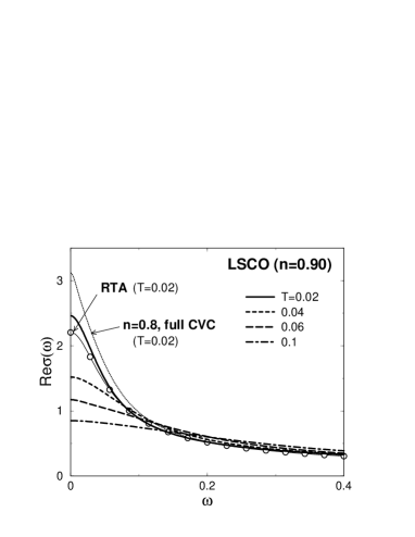
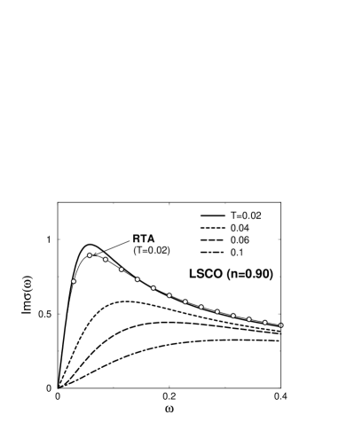
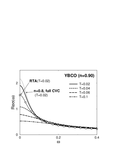
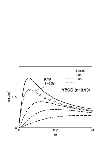
Figures 4 and 5 show the ${\omega}$-dependence of ${\sigma}({\omega})$ for LSCO ($n=0.90$) and YBCO ($n=0.90$), respectively. Both of them are qualitatively similar. Parameters for each compound are explained below eq.(4). In both cases, ${\sigma}({\omega})$ given by the CVC-FLEX approximation is slightly larger than that by RTA. In more detail, ${\sigma}({\omega})$ decreases due to the back-flow, whereas it increases due to ${\partial}\Sigma_{{\bf k}}/{\partial}k_{\mu}$ in ${\bf v}_{{\bf k}}({\epsilon})$; the latter slightly dominates in the present model parameters. Re${\sigma}({\omega})$ apparently decreases much slower than Lorentzian for larger ${\omega}$, because $\gamma_{\rm ED}({\omega})$ increases with ${\omega}$. The Drude weight is a little sharper in LSCO because a smaller value of $U$ is used. We note that the Drude weight increases as the system moves away from the half-filling ($n=1$). For LSCO at $T=0.02$, Im${\sigma}({\omega})$ takes the maximum value at ${\omega}_{xx}\sim 0.06$, which is about three times larger than $2\gamma_{{{\bf k}}_{\rm c}}(0)$ because of the ${\omega}$-dependence of $\gamma_{{{\bf k}}}({\omega})$.

Figure 6: Obtained $\sigma_{xy}({\omega})$ for LSCO by the CVC-FLEX approximation. The hight of the Drude weight is remarkably magnified by the CVC. At $T=0.02$, Re${\sigma}_{xy}({\omega})$ is negative for ${\omega}>0.3$ due to the CVC, which is consistent with experiments.

Figure 7: Obtained $\sigma_{xy}({\omega})$ for YBCO by the CVC-FLEX approximation.

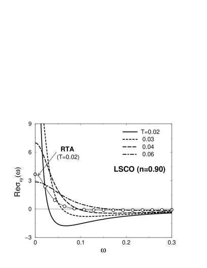
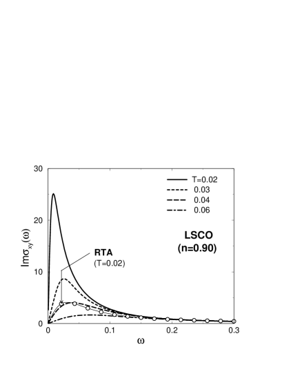
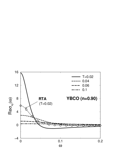
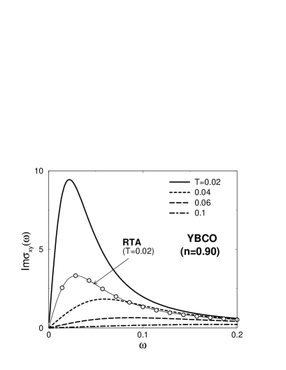
In contrast to ${\sigma}({\omega})$, ${\sigma}_{xy}({\omega})$ with full CVC is quite different from ${\sigma}_{xy}^{0}({\omega})$ given by the RTA: Figures 6 and 7 show the ${\omega}$-dependence of ${\sigma}_{xy}({\omega})$ for LSCO and YBCO, respectively. The ${\omega}$-dependence of Re${\sigma}_{xy}({\omega})$ becomes prominent due to the CVC. For LSCO (YBCO), Re${\sigma}_{xy}({\omega})$ at $T=0.02$ takes a large negative value for ${\omega}>0.03\sim 120{\rm cm}^{-1}$ (${\omega}>0.045\sim 180{\rm cm}^{-1}$), which is consistent with experimental observations Drew04 ; Drew02 ; Drew00 ; Drew00-c ; Drew96 . Although Re${\sigma}_{xy}^{0}({\omega})$ also changes its sigh for ${\omega}>0.1$, its absolute value is very small. It is naturally understood from the ED-form because $\gamma({\omega})$ increases with ${\omega}$. This large dip in Re${\sigma}_{xy}({\omega})$ is naturally understood in terms of the $f$-sum rule, eq.(80), because Re${\sigma}_{xy}(0)>0$ takes an enhanced value due to the CVC. We also stress that ${\rm Im}{\sigma}_{xy}({\omega})/{\omega}|_{{\omega}\rightarrow 0}$ is strongly enhanced due to the CVC, which is consistent with the analysis in the previous section. Later, we will discuss its temperature dependence in more detail. The overall behavior of ${\sigma}_{xy}({\omega})$ for YBCO is qualitatively similar to that for LSCO. For LSCO at $T=0.02$, Im${\sigma}_{xy}({\omega})$ takes the maximum value at ${\omega}_{xy}\sim 0.01$, which is about six times larger than ${\omega}_{xx}$ for Im${\sigma}({\omega})$.

Figure 8: Obtained $R_{\rm H}({\omega})\equiv\sigma_{xy}({\omega})/(\sigma_{xy}({\omega}))^{2}$ by the CVC-FLEX approximation. Im$R_{\rm H}({\omega})$ takes large values because the ED-form for ${\sigma}_{xy}({\omega})$ is violated due to the CVC. We note that the magnitude of $R_{\rm H}^{\rm RTA}$ in this figure is too large since the renormalization to the QP velocity by $d\Sigma_{{\bf k}}/dk_{x}$ has been dropped. The correct value is $R_{\rm H}^{\rm RTA}\;\stackrel{{\scriptstyle<}}{{\sim}}\;1$ according to ref.Kontani-Hall .

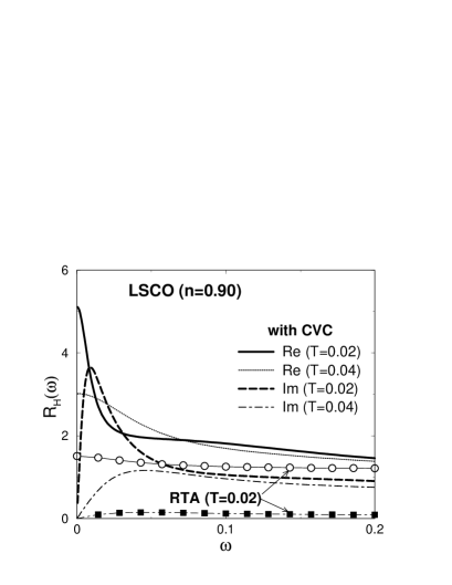
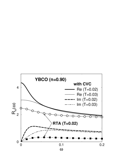
The deviation of ${\sigma}_{xy}({\omega})$ from the ED-form gives a prominent ${\omega}$-dependence of the optical Hall coefficient $R_{\rm H}({\omega})={\sigma}_{xy}({\omega})/{\sigma}^{2}({\omega})$, which is shown in fig.8. For LSCO, the ${\omega}$-dependence of $R_{\rm H}^{0}({\omega})$ given by the RTA, ${\sigma}_{xy}^{0}({\omega})/({\sigma}^{0}({\omega}))^{2}$, is very weak, and its imaginary part is tiny. This fact gives the conclusive evidence that both ${\sigma}_{xy}^{0}({\omega})$ and ${\sigma}^{0}({\omega})$ follow the ED-form. On the other hand, $R_{\rm H}({\omega})$ given by the conserving approximation shows prominent frequency as well as temperature dependences. For LSCO at $T=0.02$, Im$R_{\rm H}({\omega})$ takes the maximum value at ${\omega}_{\rm RH}\sim 0.01$, which is similar to ${\omega}_{xy}$ for Im${\sigma}_{xy}({\omega})$ and is six times larger than ${\omega}_{xx}$ for Im${\sigma}({\omega})$. The relation ${\omega}_{xx}\gg{\omega}_{xy},{\omega}_{\rm RH}$ obtained in the present study, which is consistent with experimental observation Drew04 ; Drew96 , cannot be reproduced by the RTA: It can be explained only when the back-flow is taken into account. Qualitatively similar results are obtained for YBCO, although its anomalies are more moderate. The observed $R_{\rm H}({\omega})$ in YBa₂Cu₃O₇ at 95K in ref. Drew96 looks similar to the present result for LSCO at $T=0.04$ in fig.8. The model parameters for YBCO used here may not really appropriate for a quantitative study.

In order to elucidate the reason why ${\sigma}_{xy}({\omega})$ deviates from the ED-form due to the CVC, we analyze ${\sigma}_{xy}({\omega})$ in the low frequency limit. In the RTA where CVC is absent, relations ${\sigma}_{xy}^{0}\propto\gamma_{{{\bf k}}_{\rm c}}^{-2}$ and ${\sigma}_{xy}^{0}({\omega})/i{\omega}\propto z^{-1}\gamma_{{{\bf k}}_{\rm c}}^{-3}$ are expected. As shown in fig.9 (a), following relations are held by the RTA in the present numerical study:

$${\sigma}_{xy}^{0}/({\sigma}^{0})^{2} \propto {\rm const.},$$ (73)

$${\rm Im}{\sigma}_{xy}^{0}({\omega}_{0})/({\sigma}^{0})^{3} \propto z^{-1}\propto T^{-0.4},$$ (74)

where ${\omega}_{0}$ is a small constant (${\omega}_{0}\sim 10^{-4}$). These temperature dependences is drastically changed due to the CVC, as discussed in the previous section. Actually, when the CVC’s are fully taken into account, we obtain

$${\sigma}_{xy}/{\sigma}^{2} \propto a\propto T^{-0.9},$$ (75)

$${\rm Im}{\sigma}_{xy}({\omega}_{0})/{\sigma}^{3} \propto z^{-1}b\propto T^{-1.7},$$ (76)

where coefficients $a$ and $b$ had been introduced in eq. (63). Thus, both of which are enhanced by the CVC’s as the temperature decreases. We find that ${\rm Im}{\sigma}_{xy}({\omega}_{0})/{\sigma}^{3}\propto({\sigma}_{xy}/{\sigma}^{2})^{2}$ is approximately realized in the present CVC-FLEX approximation.

Figure 9: (a) ${\sigma}_{xy}/{\sigma}_{xy}^{0}\propto T^{-0.85}$ at ${\omega}=0$ and Im${\sigma}_{xy}/{\rm Im}{\sigma}_{xy}^{0}\propto T^{-1.2}$ for small ${\omega}_{0}$. This result suggests that they are proportional to $\xi^{2}$ and $\xi^{3}$ ($\xi$ being the AF correlation length) for $T=0.03\sim 0.1$. (b) ${\sigma}_{xy}/{\sigma}^{2}\propto T^{-0.9}$ at ${\omega}=0$ and Im${\sigma}_{xy}/{\sigma}_{xy}^{3}\propto T^{-1.7}$ for small ${\omega}_{0}$.

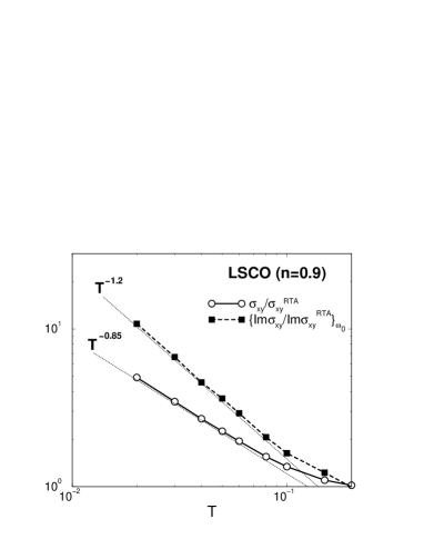
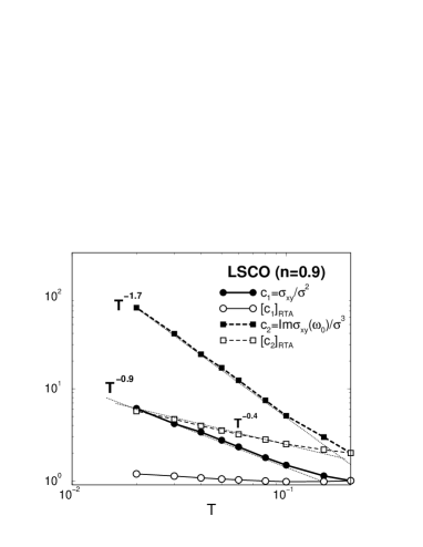
In the previous section, relations $a\propto\xi^{2}$ and $b=\xi^{m}$ ($m=2\sim 4$) are derived from the analysis of the CVC. By eqs.(73)-(76), relations $\xi^{2}\approx T^{0.9}$ and $m\approx 3$ are concluded. To confirm these results more completely, we perform another plot shown in fig. 9 (b),

$${\sigma}_{xy}/{\sigma}_{xy}^{0} \propto \xi^{2}\propto T^{-0.85},$$ (77)

$${\rm Im}{\sigma}_{xy}({\omega}_{0})/{\rm Im}{\sigma}_{xy}^{0}({\omega}_{0}) \propto \xi^{m}\propto T^{-1.2},$$ (78)

As a result, the relation $m\approx 3$ is also derived from eqs.(77) and (78). Note that the exponents of $T$ in eqs.(75) and (77) are slightly different because $({\sigma}^{0})^{2}/{\sigma}_{xy}^{0}$ shows a subtle temperature dependence.

According to eq. (66), $\lim_{{\omega}\rightarrow 0}R_{\rm H}({\omega})/i{\omega}=2z^{-1}(b-a)(2\gamma_{{{\bf k}}_{\rm c}})^{-1}$. As we discussed above, $b-a$ is positive and is enhanced as $T$ decreases. As a result, in nearly AF Fermi liquid, $i{\omega}$-linear term of $R_{\rm H}({\omega})$ is strongly enhanced by the CVC, which is consistent with experiments Drew04 ; Drew02 ; Drew00 ; Drew00-c ; Drew96 .

IV.3 $f$-sum rule

The $f$-sum rule for ${\sigma}_{\mu\nu}({\omega})$ gives a rigorous relation between the conductivity and the electron density Coleman ; Kotliar ; Yanase . It is violated in the RTA because the conservation laws are not satisfied. On the other hand, $f$-sum rule is automatically satisfied in the conservation approximation, if all the CVC’s given by the Ward identity are taken. Thus, $f$-sum rule is a useful check for the reliability of the numerical study.

The $f$-sum rules for ${\sigma}({\omega})$ and ${\sigma}_{xy}({\omega})$ in an anisotropic system are given by

$$\int_{0}^{\infty}d{\omega}{\rm Re}{\sigma}({\omega}) = \pi e^{2}\sum_{k}\frac{{\partial}^{2}{\epsilon}_{{\bf k}}}{{\partial}k_{x}^{2}}n_{{\bf k}},$$ (79)

$$\int_{0}^{\infty}d{\omega}{\rm Re}{\sigma}_{xy}({\omega}) = 0.$$ (80)

Equation (79), which can be derived directly from the Kubo formula Kubo , represents the contribution by the diamagnetic current. Equation (80) is easily recognized form the fact that ${\sigma}_{xy}({\omega})\sim|{\omega}|^{-2}$ as $|{\omega}|\rightarrow\infty$, and it is analytic in the upper-half plane of the complex ${\omega}$-space. In the case of $t^{\prime}=t^{\prime\prime}=0$, the right hand side of eq.(79) is equal to $-(\pi e^{2})\langle{\epsilon}_{{\bf k}}\rangle$, where $\langle{\epsilon}_{{\bf k}}\rangle=\sum_{{\bf k}}{\epsilon}_{{\bf k}}n_{{\bf k}}$ gives the kinetic energy.

Figure 10: $f$-sum rules both for ${\sigma}({\omega})$ and ${\sigma}_{xy}({\omega})$ are well satisfied if the CVC is correctly taken into account. This fact assures the reliability of the present numerical study.

The numerical check for the $f$-sum rule is shown in Fig. 10. Sum$\{{\rm Re}{\sigma}({\omega})\}$ and $\pi\langle{\epsilon}_{{\bf k}}^{\prime\prime}\rangle$ represent the left- and right-hand-side of eq.(79), respectively. Sum$\{{\rm Re}{\sigma}({\omega})\}$ is obtained by performing the numerical ${\omega}$-integration form 0 to 100. We see that the $f$-sum rule (79) holds well, within the relative error $\sim 2\%$. This results assure the high reliability of the present numerical study when ${\omega}$ is not so large. In general, the Pade approximation for larger ${\omega}$ is less reliable because the distance form the imaginary axis is large. On the other hand, Sum$\{{\rm Re}{\sigma}^{\rm RTA}({\omega})\}$ within the RTA (without any CVC) is smaller than the correct value, whose relative error is more than 12$\%$: This discrepancy is due to the violation of the conservation laws in the RTA.

We also plot $\displaystyle\int_{0}^{X}d{\omega}{\rm Re}{\sigma}_{xy}({\omega})/\int_{0}^{X}d{\omega}|{\rm Re}{\sigma}_{xy}({\omega})|$ in fig.10, where we put $X=100$. It should vanish identically when $X=\infty$ according to the $f$-sum rule (80) in the conserving approximation. It becomes less than 0.02 as shown in fig.10, which also suggests the high reliability of the present numerical study. This result means that the unessential poles of ${\sigma}_{xy}({\omega})$ in the upper-half-plane of the complex ${\omega}$-plane, which arises from $g^{(1)}=G^{\rm R}G^{\rm R}$ in the presence of interaction, are correctly cancelled by the vertex corrections.

The realization of $f$-sum rules confirmed in the present numerical study is better than expected, despite that all the AL-type vertex corrections are dropped. This result strongly suggests that the AL terms are insignificant for the quantitative study of ${\sigma}({\omega})$ and ${\sigma}_{xy}({\omega})$, as they are for ${\sigma}(0)$ and ${\sigma}_{xy}(0)$ Kontani-Hall .

IV.4 Inverse Hall Angle

IR optical Hall angle $\theta_{\rm H}({\omega})={\sigma}_{xy}({\omega})/{\sigma}({\omega})$ (${\omega}\raisebox{-3.22916pt}[-6.45831pt]{$\;\stackrel{{\scriptstyle<}}{{\sim}}\;$}1000{\rm cm}^{-1}=1440$K) has been intensively measured by Drew et al Drew04 ; Drew00 . They concluded that (I) Im$\theta_{\rm H}({\omega})/{\omega}$ is almost independent of ${\omega}$ and $T$, and (II) Re$\theta_{\rm H}({\omega})$ is also independent of ${\omega}$, while its $T$-dependence is large. In contrast to (I), $|{\rm Im}{\sigma}({\omega})/{\omega}|$ monotonously decreases as ${\omega}$ increases, as shown in fig. 3 (a). As a result, the Hall angle in HTSC follows a simple Drude expression IR range (${\omega}\raisebox{-3.22916pt}[-6.45831pt]{$\;\stackrel{{\scriptstyle<}}{{\sim}}\;$}1000{\rm cm}^{-1}$):

$$\theta_{\rm H}^{\rm SD}({\omega}) = \frac{\Omega_{\rm H}^{\ast}}{2\gamma_{H}^{\ast}-i{\omega}},$$ (81)

$$\gamma_{H}^{\ast} \propto T^{-d};\ \ d=1.5\sim 2$$

$$\Omega_{\rm H}^{\ast} \propto T^{0},$$

where $\gamma_{H}^{\ast}$ and $\Omega_{\rm H}^{\ast}$ are ${\omega}$-independent, In contrast, $\gamma_{\rm ED}({\omega})$ deduced from the optical conductivity is approximately $\gamma_{\rm ED}({\omega})\propto\max\{{\omega},\pi T\}$ Pines-opt : It is proportional to ${\omega}$ and is temperature-independent has a large ${\omega}$-dependence when ${\omega}>\pi T$, as recognized in fig. 3. $\Omega_{\rm H}^{\ast}$ is a constant independent of ${\omega}$ and $T$, whereas it increases as the doping decreases. This unexpected behavior of the Hall angle puts very severe constraints on theories of HTSC.

From now on, we show that such anomalous behaviors of $\theta_{\rm H}({\omega})$ in HTSC’s are well understood in terms of the Fermi liquid with strong AF fluctuations. The frequency dependence of back-flow is crucial to reproduce the correct results. Here, we mainly show numerical results only for LSCO, although similar results are also obtained for YBCO. In the present numerical study, we derive $\theta_{\rm H}({\omega})$’s from the analytic continuations of $K_{xy}(i{\omega}_{l})/(K_{xx}(i{\omega}_{l})-K_{xx}(0))$ with ${\omega}_{l}>0$, which is a analytic function on the upper-half complex ${\omega}$-plane Coleman . The value of $\theta_{\rm H}({\omega})$ obtained by this procedure is more accurate than dividing ${\sigma}_{xy}({\omega})$ by ${\sigma}({\omega})$ after the analytic continuations of $K_{xy}(i{\omega}_{l})$ and $K_{xx}(i{\omega}_{l})$ individually.

Figure 11: Obtained ${\omega}$-dependence of the inverse Hall angle for several temperatures. We see that Re$\theta_{\rm H}^{-1}$ is approximately ${\omega}$-independent for ${\omega}<0.2$ while it’s temperature dependence is large. This result, obtained by taking the CVC into account, is consistent with experiments.

Figure 12: Obtained temperature dependence of $\Omega_{\rm H}^{\ast}/\gamma_{\rm H}^{\ast}\equiv\theta_{\rm H}^{-1}(0)$ and $\Omega_{\rm H}^{\ast}\equiv-{\rm Im}\theta_{\rm H}^{-1}({\omega})/{\omega}$ for several ${\omega}$’s. $\Omega_{\rm H}^{\ast}$ is almost independent of ${\omega}$ and $T$. $\gamma_{\rm H}^{\ast}$ is insensitive to ${\omega}$, whereas it strongly depends on $T$. These behaviors of $\Omega_{\rm H}^{\ast}$ and $\gamma_{\rm H}^{\ast}$ are the most prominent experimental results.

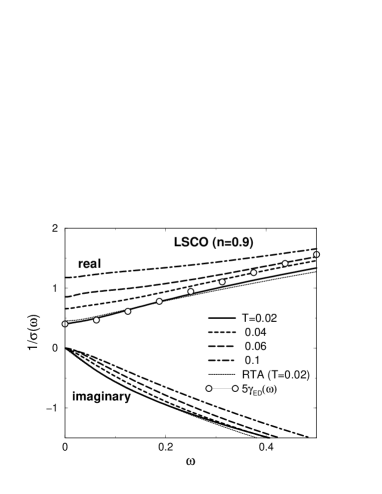
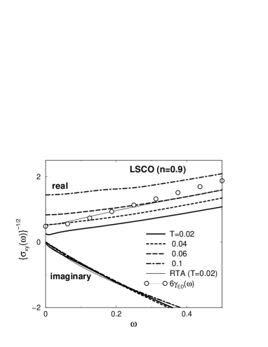
Here we discuss the inverse Hall angle by the CVC-FLEX approximation for LSCO in more detail. Figures 11 shows the ${\omega}$-dependence of $\theta_{\rm H}^{-1}({\omega})$. We can see that Re$\theta_{\rm H}^{-1}({\omega})$ given by the CVC-FLEX approximation is almost ${\omega}$-independent for ${\omega}<0.2$, which is the main experimental finding as explained above. On the other hand, Re$\{\theta_{\rm H}^{0}({\omega})\}^{-1}$ by RTA shows sizeable ${\omega}$-dependences, which is proportional to $\gamma_{\rm AV}({\omega})$ given in eq.(72). We stress that the effect of the CVC on Re$\theta_{\rm H}^{-1}({\omega})$ is prominent till frequencies much larger than $\gamma(0)$.

Figure 11 shows the imaginary part of the inverse Hall angle. Im$\theta_{\rm H}^{-1}({\omega})$ given by the CVC-FLEX approximation shows an almost complete ${\omega}$-linear behavior, and its gradient stays unchanged against the temperature ($T=0.02\sim 0.1$). On the other hand, Im$\{\theta_{\rm H}^{0}({\omega})\}^{-1}$ by the RTA shows a sub-linear behavior with respect to ${\omega}$ as shown in fig. 11, which is inconsistent with experiments. Its temperature dependence is also inconsistent, which will be shown in fig. 12. Such excess ${\omega}$- and $T$-dependences of $\{\theta_{\rm H}^{0}({\omega})\}^{-1}$ by RTA come from $z^{-1}({\omega})$, which will be discussed below.

Here we further analyze the temperature dependence of the inverse Hall angle to make comparison with experiments. Figure 12 shows obtained Re$\theta_{\rm H}^{-1}({\omega})=\Omega_{\rm H}^{\ast}/2\gamma_{H}^{\ast}$ and $(-{\rm Im}\theta_{\rm H}^{-1}({\omega})/{\omega})^{-1}=\Omega_{\rm H}^{\ast}$. Apparently, both quantities are almost ${\omega}$-independent for ${\omega}<0.2$, which confirms the experimental simple Drude expression for the Hall angle. Here, the value of $d$ in Re$\theta_{\rm H}^{-1}$ for ${\omega}<0.2$ is $d\approx 1.6$ in the present study for LSCO ($n=0.9$), whereas $d\approx 1$ by the RTA. Experimentally, $d\sim 1$ for ${\omega}\sim 1000$cm^-1 in the optimally doped YBa₂Cu₃O_6+x ($x=0.93$), and $d\sim 2$ in a slightly under-doped compound ($x=0.65$). Moreover, the value of Re$\theta_{\rm H}^{-1}({\omega})$ by CVC-FLEX approximation is much smaller than that by the RTA, which is consistent with experimental observations Drew04 ; Drew00 . We note that the value of $d$ in the DC-inverse Hall angle is approximately 2 in under-doped BSCCO exp-IHA-B and YBCO exp-IHA-Y . It slightly decreases with doping, and $d\approx 1.75$ at optimum doped systems.

Figure 12 also shows that $\Omega_{\rm H}^{\ast}$ by the CVC-FLEX approximation is almost ${\omega}$- and temperature-independent, which is consistent with experiments. Contradictory to experiments, however, it monotonously increases within the RTA. We also stress that the experimental doping dependence of $\Omega_{\rm H}^{\ast}$, which increases as the doping decreases, is reproduced well in the present study. According to eq. (67), $\lim_{{\omega}\rightarrow 0}\Omega_{\rm H}^{\ast}=za^{2}(2b-a)^{-1}$. In the RTA where $a=b=1$, we obtain $\{\Omega_{\rm H}^{0}\}^{\ast}\propto z$, which is a increase function with $T$. The inferred $T$-dependence of $\Omega_{\rm H}^{\ast}$ by RTA is recognized by the numerical study in figs. 11 and 12. If the CVC’s are taken into account, on the other hand, the temperature dependence of $\Omega_{\rm H}^{\ast}$ will be small because $\Omega_{\rm H}^{\ast}\sim za^{2}b^{-1}$ is almost constant according to eqs.(75) and (76). In fact, $\Omega_{\rm H}^{\ast}$ by the CVC-FLEX approximation is insensitive to $T$ and ${\omega}$ as shown in fig. 12. Experimental observations in HTSC’s support the results by the CVC-FLEX approximation satisfactorily.

Here we discuss experimental behavior of the Hall angle in HTSC’s in more detail. In the IR (${\omega}=900\sim 1100{\rm cm}^{-1}$) measurement Drew04 , the simple Drude form in eq.(81) is satisfied very well. It is also well recognized in YBCO, however, the extrapolation of Im$\theta_{\rm H}^{-1}$ to ${\omega}=0$ gives a positive intercept, which is recognized as a consequence of the chain contributions to ${\sigma}_{xx}$ in YBCO. Corresponding to this fact, reference Drew02 reports that the far-IR (${\omega}=20\sim 250{\rm cm}^{-1}$) Hall angle in YBa₂Cu₃O₇ deviates from eq.(81). One possible origin of this deviation other than the chain contribution would be the emergence of the pseudo-gap. In fact, DC transport coefficients show various anomalous behaviors in the pseudo-gap region. They are well reproduced theoretically in terms of the AF+SC fluctuation theory if one take the CVC into account Kontani-N . It is an important future problem to extend the scope of the present study to the pseudo-gap region, using the AF+SC fluctuation theory.

In summary, experimentally observed simple Drude form of $\theta_{\rm H}^{-1}({\omega})$ in eq.(81) is satisfactorily well reproduced by the CVC-FLEX approximation, using the parameters for LSCO. Both $\gamma_{\rm H}^{\ast}$ and $\Omega_{\rm H}^{\ast}$ are constant for ${\omega}\raisebox{-3.22916pt}[-6.45831pt]{$\;\stackrel{{\scriptstyle<}}{{\sim}}\;$}0.3$, while the former is strongly temperature dependent. Similar results are obtained even if one use parameters for YBCO, as shown in fig. 13. We note that $\theta_{\rm H}^{-1}=1.0$ in the upper panel of Fig.12 corresponds to 5000 [Tesla/radian], and $\Omega_{\rm H}^{\ast}=0.2$ in the lower panel corresponds to 0.2 [1/cm Tesla], approximately. These values seem to be well consistent with experiments Drew00 .

Figure 13: Inverse Hall angle for YBCO obtained by the CVC-FLEX approximation.

IV.5 Hall Angle

We also discuss $\theta_{\rm H}({\omega})$ given by the CVC-FLEX approximation, and make comparison with experiments. Figure 14 shows Re$\theta_{\rm H}({\omega})$ for LSCO. $\theta_{\rm H}^{0}({\omega})$ by RTA is almost temperature independent for ${\omega}>0.15$. In contrast, $\theta_{\rm H}({\omega})$ by the CVC-FLEX approximation is $T$-dependent till much larger ${\omega}$ due to the ${\omega}$-dependence of the CVC. Especially, it increases with $T$ for ${\omega}>0.15$, which is consistent with experimental observation Drew04 ; Drew00 . This change of $d{\rm Re}\theta_{\rm H}/dT$ for larger ${\omega}$ is a natural consequence of the Lorentzian form of ${\rm Re}\theta_{\rm H}({\omega})$, where $\gamma_{\rm H}$ is ${\omega}$-independent and is an increase function of temperature. In contrast, ${\rm Re}{\sigma}({\omega})$ deviates from the Lorentzian due to the ${\omega}$-dependence of $\gamma_{\rm ED}({\omega})$, which is consistent with experiments Drew04 ; Drew00 .

Figure 14: Obtained ${\omega}$-dependence of the Hall angle for several temperatures.

Figure 15: Obtained temperature dependence of the inverse Hall angle for several ${\omega}$’s. Characteristic behaviors of the experimental $\theta_{\rm H}$ are well reproduced.

The origin of the Lorentzian form of ${\rm Re}\theta_{\rm H}({\omega})$ is ascribed to the almost perfect cancellation of ${\omega}$-dependence of $\gamma_{\rm ED}({\omega})$ and that of the CVC: ${\rm Re}\theta_{\rm H}({\omega})$ for ${\omega}\gg\gamma$ will be enhances by the former effect because $\gamma_{\rm ED}({\omega})$ is a increase function of ${\omega}$, whereas it will be suppressed by the the latter, because the back-flow will be less important for larger ${\omega}$. It is a nontrivial future problem why these two effects cancel out almost completely, which results in the observed Lorentzian form of ${\rm Re}\theta_{\rm H}({\omega})$ for ${\omega}\raisebox{-3.22916pt}[-6.45831pt]{$\;\stackrel{{\scriptstyle<}}{{\sim}}\;$}1000{\rm cm}^{-1}$.

Figure 15 shows the temperature dependences of $\theta_{\rm H}({\omega})$ for several ${\omega}$’s. The obtained results for ${\omega}=0.2$ or $0.4$ look similar to the experimental observations for YBCO with $x=0.93$ (optimum) or $x=0.65$ (slightly under-doped) for ${\omega}\sim 1000{\rm cm}^{-1}$ Drew04 . On the other hand, the result for ${\omega}=0.04$ resembles the observation for heavily under-doped non-superconducting sample ($x=0.4$). We guess from this fact that the electronic states in heavily under-doped systems are qualitatively reproduced, although the experimental value of $\gamma_{\rm H}^{\ast}$ is much larger.

IV.6 Predictions for Electron-Doped Systems

DC transport phenomena under magnetic field in electron-doped systems (e.g., NCCO) also shows striking NFL behaviors which originate from the CVC Kontani-Hall ; Kontani-S . Surprisingly, both $R_{\rm H}$ and $S$ in a under-doped NCCO is negative, and its absolute value increase as $T$ decreases. Their behavior looks approximately symmetrical to those in hole-doped systems. Contrary to these experimental facts, the RTA predicts the positive Hall coefficient because it has a hole-like FS whose shape is similar to YBCO. This discrepancy is naturally solved if one take the CVC into account, since ${\partial}\theta^{J}/{\partial}k_{\parallel}$ becomes positive around the cold spot of NCCO whose location is different from that of YBCO; see fig.1 (a) Kontani-Hall .

Figure 16: Obtained $\sigma({\omega})$, $\sigma_{xy}({\omega})$ and $R_{\rm H}({\omega})$ for NCCO by the CVC-FLEX approximation.

Quite recently, optical Hall conductivity in electron-doped systems has been observed by Zimmers et al Zimmers . Here, we analyze the ${\omega}$-dependences of ${\sigma}_{\mu\nu}({\omega})$ in electron-doped systems based on the conserving approximation. Figure 16 shows ${\sigma}({\omega})$, ${\sigma}_{xy}({\omega})$ and $R_{\rm H}({\omega})$ obtained by the CVC-FLEX approximation. Both ${\sigma}_{xy}({\omega})$ and $R_{\rm H}({\omega})$ for NCCO are similar to those for LSCO given in Figs. 6 and 8, except their signs. We stress that Im$R_{\rm H}({\omega})$ is as large as Re$R_{\rm H}({\omega})$ for finite ${\omega}$, which means that the simple ED-form of ${\sigma}_{xy}({\omega})$ is violated. We predict that the signs of Re$R_{\rm H}({\omega})$ and Re${\sigma}_{xy}({\omega})$ change from negative to positive with ${\omega}$. Thus, the CVC in NCCO plays important roles. In future, measurements of ${\sigma}_{xy}({\omega})$ in NCCO are highly anticipated.

We found that an accurate numerical calculation (Pade approximation) for NCCO is much difficult than that for LSCO and YBCO. By this reason, we could not obtain reliable results for $0.04\raisebox{-3.22916pt}[-6.45831pt]{$\;\stackrel{{\scriptstyle>}}{{\sim}}\;$}T\raisebox{-3.22916pt}[-6.45831pt]{$\;\stackrel{{\scriptstyle>}}{{\sim}}\;$}0.08$. It is a future important problem to improve the stability of the Pade approximation in case of NCCO.

V Summary and Future problems

In the present work, we have calculated the optical conductivities ${\sigma}({\omega})$ and ${\sigma}_{xy}({\omega})$ for HTSC’s by the CVC-FLEX approximation. Experimentally observed anomalous behaviors for ${\sigma}({\omega})$, ${\sigma}_{xy}({\omega})$, $\theta_{\rm H}({\omega})$ and $R_{\rm H}({\omega})$ are well reproduced for enough wide range of frequencies and temperatures, without assuming any fitting parameters Letter . Especially, (I) ${\sigma}({\omega})$ given by the CVC-FLEX approximation follows the ED-form shown in eq. (70) with the relaxation time in eq. (72), whereas ${\sigma}_{xy}({\omega})$ strongly deviates from the ED-form, eq. (71), because the ${\omega}$-dependence is much exaggerated due to the CVC in nearly AF Fermi liquids. By this reason, (II) Im$R_{\rm H}({\omega})\sim{\rm Re}R_{\rm H}({\omega})$ is realized even when for ${\omega}\ll\gamma$, as shown in Fig. 8. Moreover, (III) $\theta_{\rm H}({\omega})$ follows a simple Drude form given in eq.(81) for ${\omega}\raisebox{-3.22916pt}[-6.45831pt]{$\;\stackrel{{\scriptstyle<}}{{\sim}}\;$}0.2$, as shown in Figs. 11, 12 and 13. They are consistent with the characteristic experimental results for HTSC’s reported by Drew et al. Drew96 ; Drew00 ; Drew04 . These anomalous AC transport phenomena cannot be reproduced by previous theoretical works based on the RTA, even if one assume extremely anisotropic $\tau_{{\bf k}}$. Instead, they are naturally explained by taking the CVC into account in accordance with the Ward identity.

In the present study, we have pointed out the important role of the back-flow in the optical conductivities for the first time. The enhancement of ${\rm Im}{\sigma}_{xy}({\omega})/i{\omega}|_{{\omega}=0}$ due to the CVC is not same as the enhancement of ${\sigma}_{xy}(0)$; The former is more prominent than the latter as explained in eqs.(75)-(78). This fact leads to the breakdown of the extended Drude-form at very low frequencies. The back-flow decreases monotonically with ${\omega}$ as one approaches the collisionless region (${\omega}\raisebox{-3.22916pt}[-6.45831pt]{$\;\stackrel{{\scriptstyle>}}{{\sim}}\;$}\gamma$). This fact gives an approximate Drude-form of the Hall angle in eq.(81) for ${\omega}\raisebox{-3.22916pt}[-6.45831pt]{$\;\stackrel{{\scriptstyle<}}{{\sim}}\;$}0.2$, nonetheless of the fact that ${\sigma}({\omega})$ deviates from a simple Drude-form (instead it follows a ED-form) due to the ${\omega}$-dependence of $\gamma({\omega})$. Note that the back-flow in the collisionless region is given by the real part of ${\cal T}_{22}$ Eliashberg ; Okabe ; Jujo . This is an important future problem for us to find a simple physical explanation for this numerical result.

We stress that both AC and DC anomalous transport phenomena in HTSC’s are explained in a unified way based on the Fermi liquid theory, if one take the CVC to satisfy the conservation laws. As for the DC Hall coefficient, one frequently attribute the enhancement of $R_{\rm H}$ to the small area of the cold spot (Fermi arc) observed by ARPES in under-doped compounds. However, this idea contradicts the fact that the $R_{\rm H}$ decreases in the pseudo-gap region while the Fermi arc shrinks further. In the same way, anomalous behaviors of $\Delta\rho/\rho$, $S$ and $\nu$ in the pseudo-gap region cannot be understood within the scheme of the RTA. Such contradictions are satisfactorily solved by the CVC-FLEX approximation, by taking the superconducting fluctuations induced by the AF fluctuations Kontani-N . We stress that the natural extension of this DC transport theory to AC transport phenomena, with taking the same diagrams for the CVC, succeeds in explaining the optical Hall effect observed in HTSC’s. This fact means that the qualitative dynamical electronic properties of HTSC’s, from the over-doped to the slightly under-doped systems, are well understood in terms of the Fermi liquid theory with strong AF fluctuations.

There remain many important issues for the Future study. For example, one can study various AC-transport coefficients other than ${\sigma}_{\mu\nu}$ based on the CVC-FLEX approximation, using the similar method developed in the present study. Study of the role of the CVC at finite frequencies for $\Delta\rho/\rho$, $S$ and $\nu$ would be very interesting, although experimental observation would be difficult at the present stage. In addition, we are planning to study the optical conductivities in the pseudo-gap region based on the FLEX+T-matrix approximation, which ascribes the pseudo-gap phenomena in HTSC’s to the strong superconducting fluctuations Yamada-rev . As we mentioned in the previous section, reference Drew02 reports that the far-IR (${\omega}=20\sim 250{\rm cm}^{-1}$) Hall angle in YBa₂Cu₃O₇ deviates from the Drude-form in eq.(81), although it is well satisfied for ${\omega}\sim 1000{\rm cm}^{-1}$. We would like to find out whether such an anomaly in far-IR Hall angle could be understood as the pseudo-gap effect using the AF+SC fluctuation theory.

Appendix A Physical Meaning of the Back-Flow

Throughout the present work, we have stressed the importance of the back-flow for both DC and AC transport phenomena. Here, we would like to depict the physical aspect of the back-flow in nearly AF Fermi liquid based on the phenomenological Landau-Fermi liquid theory Nozieres . According to Landau, the energy of the quasiparticle ${\tilde{\epsilon}}_{{{\bf k}}{\sigma}}$ is expressed as

$${\tilde{\epsilon}}_{{{\bf k}}{\sigma}}={{\epsilon}}_{{{\bf k}}{\sigma}}+\sum_{{{\bf k}}^{\prime}{\sigma}^{\prime}}f_{{{\bf k}}{\sigma},{{\bf k}}^{\prime}{\sigma}^{\prime}}\delta n_{{{\bf k}}^{\prime}{\sigma}^{\prime}}+O((\delta n)^{2}),$$ (82)

where ${{\epsilon}}_{{{\bf k}}{\sigma}}={{\bf k}}^{2}/2m^{\ast}$, $n_{{{\bf k}}{\sigma}}$ is the distribution function of quasiparticles, $f_{{{\bf k}}{\sigma},{{\bf k}}^{\prime}{\sigma}^{\prime}}$ is the Landau function, and $\delta n_{{{\bf k}}{\sigma}}=n_{{{\bf k}}{\sigma}}-n_{{{\bf k}}{\sigma}}^{T=0}$. Equation (82) means that the energy of quasiparticles are changed when the quasiparticle excitation exists. By this reason, once we add a quasiparticle at ${{\bf k}}$ outside the FS, the Fermi sphere is deformed to minimize the total energy unless $f_{{{\bf k}}{\sigma},{{\bf k}}^{\prime}{\sigma}^{\prime}}=0$. As a result, the Fermi sphere has a finite momentum, which is the physical meaning of the back-flow. Thus, the existence of the back-flow is assured by the most essential relation in the Fermi liquid, eq.(82). Apparently, the back-flow would be indispensable in strongly correlated Fermi liquids, like in HTSC.

The importance of the back-flow has been understood very well in a spherical system, where $f_{{{\bf k}}{\sigma},{{\bf k}}^{\prime}{\sigma}^{\prime}}$ can be expanded by Legendre polynomials, $P_{l}({\hat{{\bf k}}}\cdot{\hat{{\bf k}}^{\prime}})$. Landau first studied the back-flow in the collisionless region ${\omega}\gg\gamma$, where the lifetime of an quasiparticles is longer than the period of the outer field. Based on the Kubo formula, Yamada and Yosida analyzed the opposite region ${\omega}\ll\gamma$ in order to study the role of the back-flow on the DC conductivity. They rigorously proved that the conductivity diverges even at finite temperatures if no Umklapp scattering process exists. In contrast, the RTA always gives finite conductivity ${\sigma}\propto\gamma^{-1}$ at $T\neq 0$ even in the absence of the Umklapp process, reflecting the the violation of the momentum conservation laws.

In contrast, importance of the back-flow in anisotropic systems with strong correlations has not been recognized until recently. As explained in §III, we found that total current ${\bf J}_{{\bf k}}$ becomes quite different from the quasiparticle velocity ${\bf v}_{{\bf k}}$ due to the CVC when the AF fluctuations with ${{\bf q}}\approx{\bf Q}$ are strong Kontani-Hall . This is the origin of various anomalous transport phenomena in HTSC’s. This unexpected behavior of ${\bf J}_{{\bf k}}$ comes from the fact that ${\cal T}_{22}({{\bf k}}-{{\bf k}}^{\prime})$ in the Bethe-Salpeter equation (50), which corresponds to the Landau function for ${\omega}\ll\gamma$, takes large values only for ${{\bf k}}-{{\bf k}}^{\prime}\approx{\bf Q}$. In this case, according to eq.(82), a quasiparticle added at ${{\bf k}}^{\prime}$ strongly modifies ${\tilde{\epsilon}}_{{\bf k}}$ only when ${{\bf k}}\approx{{\bf k}}^{\prime}+{\bf Q}$, which makes the induced current (back-flow) proportional to ${\bf v}_{{{\bf k}}}$. The induced current is not parallel to the source velocity ${\bf v}_{{{\bf k}}^{\prime}}$, in contrast to the case of spherical systems. The schematic behavior of ${\bf J}_{{\bf k}}$ in HTSC’s is shown in fig.1 (b). ${\bf J}_{{\bf k}}$ at the hot spot takes enhanced values because ${\alpha}_{{\bf k}}\raisebox{-3.22916pt}[-6.45831pt]{$\;\stackrel{{\scriptstyle<}}{{\sim}}\;$}1$ in eq.(52), which is interpreted as the “resonance” between ${\bf v}_{{\bf k}}$ and ${\bf v}_{{{\bf k}}^{\prime}}$.

In the present paper, we studied the optical conductivity and Hall conductivity by taking the ${\omega}$-dependence of the CVC into account appropriately, which has not been performed in previous studies. We find that ${\sigma}_{xy}({\omega})$ shows a striking ${\omega}$-dependence when the AF fluctuations are strong, which cannot be expressed by an ED-form. Such a non-Fermi liquid-like behavior comes from the prominent ${\omega}$-dependence of the CVC, which was detected in the present study for the first time. As shown in §III, the total current at finite ${\omega}$ is given by ${\bf J}_{{\bf k}}({\omega})={\bf J}_{k}+i{\omega}{\bf J}_{k}^{(1)}+O({\omega}^{2})$, where ${\bf J}_{k}^{(1)}$ is real and its ${{\bf k}}$-dependence is much larger than the first term. This strong ${\omega}$-dependence of the total current gives rich variety of spectrum in optical conductivities.

Appendix B Comments on Previous Theoretical Studies

Anomalous DC transport phenomena in HTSC’s, as represented by the enhancement of the Hall coefficient, have been frequently ascribed to the reduction of the effective carrier number within the RTA. For example, Ref. Pines-Hall proposed the highly anisotropic $\tau_{{\bf k}}$ model based on a spin fluctuation theory; $\tau_{\rm h}\propto T^{-1}$ for hot electrons whose density is $n_{\rm h}$, $\tau_{\rm c}\propto T^{-2}$ for cold electrons whose density is $n_{\rm c}(=n-n_{\rm h})$. They assume that $n_{\rm c}\ll n_{\rm h}$ and $\tau_{\rm c}/\tau_{\rm h}\sim 100$ at lower temperatures. Their model cannot give a comprehensive explanation for anomalous DC transport phenomena in HTSC’s, while the CVC-FLEX approximation can give it.

Here, we examine the optical conductivities within the RTA based on a simplified anisotropic $\gamma_{{\bf k}}$ model as follows:

$${\sigma}({\omega}) \propto \frac{n_{\rm c}}{2\gamma_{\rm c}-i{\omega}}+\frac{n_{\rm h}}{2\gamma_{\rm h}-i{\omega}},$$ (83)

$${\sigma}_{xy}({\omega}) \propto \frac{n_{\rm c}}{(2\gamma_{\rm c}-i{\omega})^{2}}+\frac{n_{\rm h}}{(2\gamma_{\rm h}-i{\omega})^{2}},$$ (84)

where $\tau_{\rm h,c}=1/2\gamma_{\rm h,c}$. The Hall coefficient is highly enhanced in proportion to $1/en_{\rm c}(\propto T^{-1})$ when $n_{\rm c}/\gamma_{\rm c}^{2}\gg n_{\rm h}/\gamma_{\rm h}^{2}$.

In the case of $n_{\rm c}\ll n_{\rm h}$ and $\gamma_{\rm c}\ll\gamma_{\rm h}$, frequencies ${\omega}_{xx}$, ${\omega}_{xy}$ and ${\omega}_{\rm RH}$ which give the maximum Im${\sigma}({\omega})$, Im${\sigma}_{xy}({\omega})$ and Im$R_{\rm H}({\omega})$ respectively, are given by

$${\omega}_{xx} = 2\gamma_{\rm c},$$ (85)

$${\omega}_{xy} = (2/\sqrt{3})\gamma_{\rm c}=1.16\gamma_{\rm c},$$ (86)

$${\omega}_{\rm RH} = \frac{2(\gamma_{\rm c}n_{\rm h}+\gamma_{\rm h}n_{\rm c})}{\sqrt{3}n_{\rm h}},$$ (87)

where ${\omega}_{\rm RH}$ is approximately given by

$${\omega}_{\rm RH} \approx 1.16n_{\rm c}\gamma_{\rm h}/n_{\rm h}\gg\gamma_{\rm c}\ \ \ \ \ \ {\rm for}\ {n_{\rm c}}/{\gamma_{\rm c}}\gg{n_{\rm h}}/{\gamma_{\rm h}},$$

$$\approx 2.31\gamma_{\rm c}\ \ \ \ \ \ \ \ \ \ \ \ \ \ \ \ \ \ \ \ \ {\rm for}\ {n_{\rm c}}/{\gamma_{\rm c}}={n_{\rm h}}/{\gamma_{\rm h}},$$

$$\approx 1.16\gamma_{\rm c}\ \ \ \ \ \ \ \ \ \ \ \ \ \ \ \ \ \ \ \ \ {\rm for}\ {n_{\rm c}}/{\gamma_{\rm c}}\ll{n_{\rm h}}/{\gamma_{\rm h}}.$$

Because ${n_{\rm c}}/{\gamma_{\rm c}}(\propto T^{-3})$ will be larger than ${n_{\rm h}}/{\gamma_{\rm h}}(\propto T^{-1})$ at lower temperatures, the relation ${\omega}_{\rm RH}\raisebox{-3.22916pt}[-6.45831pt]{$\;\stackrel{{\scriptstyle>}}{{\sim}}\;$}{\omega}_{xx}$ is expected in this model. This result is inconsistent with experimental fact ${\omega}_{\rm RH}\ll{\omega}_{xx}$, as mentioned in §I.

In a similar way, d-density wave (DDW) model DDW have been proposed to explain the enhancement of of the Hall coefficient: $R_{\rm H}$ increases below the d-density wave transition temperature, inversely proportional to the area of the “Fermi arc”. However, it is hopeless to reproduce the characteristic experimental behavior of $R_{\rm H}({\omega})$ in this model.

We also comment on the 2D Luttinger liquid model with two kinds of relaxation times ($\tau_{\rm tr}\propto T^{-1}$, $\tau_{\rm H}\propto T^{-2}$) proposed by Anderson Anderson . In this model, DC conductivities are given by ${\sigma}\propto\tau_{\rm tr}^{-1}$ and ${\sigma}_{xy}\propto(\tau_{\rm tr}\tau_{\rm H})^{-1}$, respectively. Their natural extensions to the optical conductivities are given as ${\sigma}({\omega})\propto(\tau_{\rm tr}^{-1}-i{\omega})^{-1}$ and ${\sigma}_{xy}({\omega})\propto(\tau_{\rm tr}/\tau_{\rm H}){\sigma}^{2}({\omega})$ Romero . This result directly means that Im$R_{\rm H}({\omega})\equiv 0$, which apparently contradicts experiments. In addition, the Hall angle in this model is $\theta_{\rm H}({\omega})\propto(\tau_{\rm tr}/\tau_{\rm H})\cdot(\tau_{\rm tr}^{-1}-i{\omega})^{-1}$; the temperature dependences of coefficients are different from the experimental ones given in eq.(81). Note that another functional form of ${\sigma}_{\mu\nu}({\omega})$ which predict finite Im$R_{\rm H}({\omega})$ was proposed in ref. Drew96 , although its theoretical verification is uncertain.

In summary, a comprehensive understanding for the optical Hall coefficient in HTSC’s cannot be obtained by previous theoretical works based on the RTA, or by the 2D Luttinger liquid theory. The transport theory based on the Fermi liquid theory presented in the present paper, where the CVC is correctly taken into account, can explain various experimental anomalies at the same time.

References

- (1) Y. Yanase, T. Jujo, T. Nomura, H. Ikeda, T. Hotta and K. Yamada: Phys. Rep. 387 (2003) 1.
- (2) T. Moriya and K. Ueda: Adv. Physics 49 (2000) 555.
- (3) P. Monthoux and D. Pines: Phys. Rev. B 47 (1993) 6069.
- (4) H. Kontani and K. Yamada: J. Phy. Soc. Jpn. 74 (2005) 155.
- (5) N. E. Bickers and S. R. White: Phys. Rev. B 43 (1991) 8044.
- (6) P. Monthoux and D. J. Scalapino, Phys. Rev. Lett. 72 (1994) 1874.
- (7) J. Takeda, T. Nishikawa, and M. Sato: Physica C 231 (1994) 293.
- (8) T. Kimura, S. Miyasaka, H. Takagi, K. Tamasaku, H. Eisaki, S. Uchida, K. Kisazawa, M. Hiroi, M. Sera, and N. Kobayashi: Phys. Rev. B 53 (1996) 8733.
- (9) Y. Ando and T. Murayama : Phys. Rev. B 60 (1999) R6991; Y. Ando and K. Segawa: Phys. Rev. Lett. 88 (2002) 167005.
- (10) L.B. Ioffe and A. J. Millis: Phys. Rev. B 58 (1998) 11631.
- (11) H. Kontani: J. Phys. Soc. Jpn. 70 (2001) 1873.
- (12) H. Kontani, K. Kanki and K. Ueda: Phys. Rev. B 59 (1999) 14723, K. Kanki and H. Kontani: J. Phys. Soc. Jpn. 68 (1999) 1614.
- (13) H. Kontani: J. Phys. Soc. Jpn. 70 (2001) 2840.
- (14) H. Kontani: Phys. Rev. Lett. 89 (2003) 237003.
- (15) L. B. Rigal, D. C. Schmadel, H. D. Drew, B. Maiorov, E. Osquiguil, J. S. Preston, R. Hughes, and G. D. Gu: Phys. Rev. Lett. 93 (2004) 137002.
- (16) M. Grayson, L. B. Rigal, D. C. Schmadel, H. D. Drew, and P.-J. Kung: Phys. Rev. Lett. 89 (2002) 037003.
- (17) J. Cerne, M. Grayson, D. C. Schmadel, G. S. Jenkins, H. D. Drew, R. Hughes, A. Dabkowski, J. S. Preston, and P.-J. Kung: Phys. Rev. Lett. 84 (2000) 3418.
- (18) J. Cerne, D. C. Schmadel, L. B. Rigal, H. D. Drew: cond-mat/0210325.
- (19) S.G. Kaplan, S.Wu, H.-T.S. Lihn, H.D. Drew, Q. Li, D.B. Fenner, J.M. Phillips and S.Y. Hou: Phys. Rev. Lett. 76 (1996) 696.
- (20) J. Cerne, D.C. Schmadel, M. Grayson, G.S. Jenkins, J.R. Simpson and H.D. Drew: Phys. Rev. B 61 (2000) 8133.
- (21) A. Zimmers, L. Shi, D.C. Schmadel, R.L. Greene and H.D. Drew, cond-mat/0510085.
- (22) H. Kontani: cond-mat/0507664.
- (23) B.P. Stojković and D. Pines: Phys. Rev. B 56 (1997) 11931.
- (24) A. Georges, G. Kotliar, W. Krauth, and M. J. Rozenberg: Rev. Mod. Phys. 68 (1996) 13.
- (25) G. Kotliar and D. Vollhardt: Physics Today 57 (2004) 53.
- (26) T. Okabe: J. Phys. Soc. Jpn 67 (1998) 2792.
- (27) T. Jujo: J. Phys. Soc. Jpn 70 (2001) 1349, T. Jujo: J. Phys. Soc. Jpn 71 (2002) 888.
- (28) G. Baym and L.P. Kadanoff: Phys. Rev. 124 (1961), 287.
- (29) G. Baym: Phys. Rev. 127 (1962), 1391.
- (30) H. Kino and H. Kontani: J. Phys. Soc. Jpn. 67 (1998) 3691.
- (31) H. Kondo and T. Moriya: J. Phys. Soc. Jpn. 67 (1998) 3695.
- (32) J. Schmalian: Phys. Rev. Lett. 81 (1998) 4232.
- (33) H. Kontani and H. Kino: Phys. Rev. B 63 (2001) 134524.
- (34) R. Hlubina and T. M. Rice: Phys. Rev. B 51 (1995) 9253.
- (35) B.P. Stojković and D. Pines: Phys. Rev. B 55 (1996) 857.
- (36) N. P. Armitage, D. H. Lu, C. Kim, A. Damascelli, K. M. Shen, F. Ronning, D. L. Feng, P. Bogdanov, Z.-X. Shen, Y. Onose, Y. Taguchi, Y. Tokura, P. K. Mang, N. Kaneko, and M. Greven: Phys. Rev. Lett. 87 (2001), 147003.
- (37) N. P. Armitage, F. Ronning, D. H. Lu, C. Kim, A. Damascelli, K. M. Shen, D. L. Feng, H. Eisaki, Z.-X. Shen, P. K. Mang, N. Kaneko, M. Greven, Y. Onose, Y. Taguchi, and Y. Tokura: Phys. Rev. Lett. 88 (2002), 257001.
- (38) G. M. Eliashberg : Sov. Phys. JETP 14 (1962), 886.
- (39) H. Kohno and K. Yamada: Prog. Theor. Phys. 80 (1988) 623.
- (40) H. Fukuyama, H. Ebisawa and Y. Wada: Prog. Theor. Phys. 42 (1969) 494.
- (41) H. Kontani: Phys. Rev. B 64 (2001) 054413.
- (42) H. Kontani: Phys. Rev. B 67 (2003) 014408.
- (43) H. D. Drew and P. Coleman: Phys. Rev. Lett. 78 (1997) 1572.
- (44) E. Lange and G. Kotliar: Phys. Rev. Lett. 82 (1999) 1317.
- (45) Y. Yanase and M. Ogata: cond-mat/0412508.
- (46) R. Kubo: J. Phys. Soc. Jpn. 12 (1957) 570.
- (47) Z. Konstantinovic, Z. Z. Li, and H. Raffy: Phys. Rev. B 62 (2000) R11989.
- (48) H.Y. Hwang, B. Batlogg, H. Takagi, H. L. Kao, J. Kwo, R. J. Cava, J.J. Krajewski, and W.F. Peck, Jr.: Phys. Rev. Lett. 72 (1994) 2636.
- (49) D. Pines and P. Nozieres: The theory of Quantum Liquids (W.A. Benjamin, New York, 1966.)
- (50) S. Chakravarty, C. Nayak, S. Tewari, and X. Yang: Phys. Rev. Lett. 89 (2002) 277003.
- (51) P.W. Anderson: Phys. Rev. Lett. 67 (1991) 2092.
- (52) D.B. Romero: Phys. Rev. B 46 (1992) 8505.