Efficient evaluation of decoherence rates in complex Josephson circuits
Abstract
A complete analysis of the decoherence properties of a Josephson junction qubit is presented. The qubit is of the flux type and consists of two large loops forming a gradiometer and one small loop, and three Josephson junctions. The contributions to relaxation () and dephasing () arising from two different control circuits, one coupled to the small loop and one coupled to a large loop, is computed. We use a complete, quantitative description of the inductances and capacitances of the circuit. Including two stray capacitances makes the quantum mechanical modeling of the system five dimensional. We develop a general Born-Oppenheimer approximation to reduce the effective dimensionality in the calculation to one. We explore and along an optimal line in the space of applied fluxes; along this “S line” we see significant and rapidly varying contributions to the decoherence parameters, primarily from the circuit coupling to the large loop.
pacs:
03.67.Lx, 03.65.Yz, 5.30.-dI Introduction
Recent years have seen many successes in obtaining high-coherence quantum behavior in a variety of flux-based Josephson-junction qubits. The devices which show good behavior as qubits are fairly complex electrical circuits, and a detailed theoretical analysis of these circuits has proven useful in arriving at optimal designs with the best decoherence behaviorB1 ; B2 . Since the first reports of coherent oscillations in Josephson qubitsNakamura , the observed coherence times have increased by a factor of about 5000; theory has had a substantial role in this large increase (for a theoretical review of Josephson qubits, see Makhlin ), by suggesting strategies for choosing optimal settings of control parameters for the operation of the qubit.
In this paper, we report the results of a detailed theoretical study of the flux qubit recently reported by our groupKochetal . We will make extensive use of a method of analysis introduced by Burkard, Koch, and DiVincenzo (BKD)BKD . BKD introduced a universal method for analyzing any electrical circuit that can be represented by lumped elements. BKD proceeds in several steps: first, the Kirchhoff equations are formulated in graph theoretic language so that they describe the dynamics of a general circuit in terms of a set of independent, canonical coordinates. Then, one set of terms in these equations of motion (the “lossless” part) is seen to be generated by a Hamiltonian describing a massive particle in a potential; the number of space dimensions in which the particle moves is equal to the number of canonical coordinates in the Kirchhof equations. The “lossy” parts of the equations of motion are treated by introducing a bath of harmonic oscillators, in the style of Caldeira and LeggettCG .
Finally the resulting total Hamiltonian, involving a system, a bath, and a system-bath coupling, can be analyzed by standard means to determine the decoherence parameters, and , of the first two eigenlevels of the system (the “qubit”). is the energy loss rate of the qubit, while , the “pure dephasing time”, is related to the experimental parameter , the decay time of Ramsey fringes, by . Long and times are both necessary conditions for quantum computing.
The results of this paper have revealed significant facts about the dependence of and on the control parameters of our qubit. The qubit has, to a good degree of approximation, a bilateral symmetry across its midline (see Fig. 1). This symmetry manifests itself in the quantum behavior: The quantum structure is effectively that of a symmetric double well potential whenever the difference of bias fluxes in the two large loops is the flux quantum . (The structure is a “gradiometer”, meaning that, to good approximation, its behavior is only a function of the difference of the magnetic flux in the two large loops.)
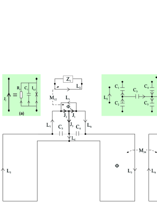
We will analyze the decoherence parameters arising from the two impedances shown, and . Because is coupled to the qubit via the “small” loop, we refer to the decoherence parameters associated with it as and ; the corresponding parameters for , coupled via the “large” loop, are and . We find that the bilateral symmetry completely controls the overall structure of the s and s. All these parameters are symmetric in around ( and are approximately symmetric for small values of control flux , the other two are exactly symmetric). Furthermore, , , and all have divergent behavior at the symmetric point; is exactly divergent, and are very nearly so for a large range of small-loop control flux . These facts give a powerful motivation for operating the qubit always very near . As a function of , is strongly increasing and is strongly decreasing (in the symmetric situation). This makes it essential to stay within a particular window of operating parameters.
As we will discuss in detail, the full dependence of the four decoherence parameters on and is complex, but can be grossly understood as being controlled by two distinct regimes, the “semiclassical” and the “harmonic”. In the semiclassical regime, the effective potential is a double well with a high barrier between, so that quantum tunneling is very small. As is increased, the barrier drops, then disappears altogether; then the qubit potential enters the “harmonic” regime, where the potential is approximately just a single, quadratic well. These two extreme cases are relatively simple; decoherence in the regime of crossover between these two is rather complex.
We gain some further insight into these results via a technical improvement that we have added to the analysis of BKDBKD . A description of this improvement, an application of the Born-Oppenheimer approximation, is another important component of this paper. This improvement was motivated by the fact that we wanted to study the effect of stray capacitances in the qubit circuit of Fig. 1. The quantum mechanics that this model defines is that of a particle in a five-dimensional potential (five because there are three junction capacitances and two stray capacitances, each defining a degree of freedom). A direct evaluation of the Schroedinger equation in five dimensions is numerically complex. But we find that, in a controlled way, we can organize these five dimensions into four coordinate directions that are “fast” (in which the potential rises very steeply) and one that is “slow” (and has the double-well structure at low ). Then, just as in molecular physics Mertzbacher , the fast coordinates can be treated adiabatically, having the effect of modifying the effective slow potential energy in the one remaining coordinate. The resulting one-dimensional quantum theory is very easy to analyze numerically, and amenable to a qualitative discussion.
This paper is organized as follows: Sec. II introduces the network graph formalism that we use to analyze the quantum mechanics of Josephson circuits. We stress two innovations that considerably streamline the analysis: a capacitance rescaling, and a Born-Oppenheimer approximation. The Appendix gives more background about the theory, with subsection A giving a review, with some minor corrections, of the relevant parts of BKDBKD , and subsection B highlighting some new results in network graph theory. Sec. III discusses the details of the necessary computation that are specific to the gradiometer qubit. Sec. IV gives a qualitative discussion of the features of the four decoherence parameters, , , , and that we compute. Sec. V reviews a semiclassical analysis from BKDBKD that is helpful in understanding the overall features of the decoherence parameters. The four Secs. VI-IX give an extended discussion of each of the four decoherence parameters. Sec. X gives some conclusions.
II Analysis: capacitance rescaling and Born Oppenheimer approximation
Our analysis follows closely that of BKDBKD . A summary of the essentials of this theory is given in Appendix A. The result of this theory is, first, a system Hamiltonian, which we begin with here (see Eq. (86)):
| (1) |
| (2) |
To perform the Born Oppenheimer approximation, it is best to first go to a rescaled coordinate system in which the mass (i.e., the capacitance matrix ) is isotropic. This is mentioned in BKDBKD , but we present this analysis more generally here to set our notation. We make the following coordinate transformation
| (3) | |||
| (4) |
is some standard capacitance; it is convenient to insert this arbitrary number so that and f have the same units as and , respectively. Note that the commutation relations are left unchanged by this coordinate change:
| (5) |
The Hamiltonian for the rescaled Schroedinger equation is
| (6) |
| (7) | |||||
For computing decoherence parameters, we take over unchanged the golden-rule formulas discussed in BKDBKD (see Appendix):
| (8) | |||||
| (9) |
For the rescaled coordinates, these are
| (10) | |||||
| (11) |
We will discuss the use of the Born-Oppenheimer approximation to evaluate these formulas. What must be computed are matrix elements of the form
| (12) |
where , and is the constant vector .
As discussed in the introduction, we single out one (more than one is also possible) “slow” degree of freedom , and take all coordinate directions orthogonal to this one, , to be “fast”. So
| (13) |
The fast coordinates are characterized by the fact that the potential increases very rapidly in the -direction; we assume that it is a good approximation to expand in these directions to second order:
| (14) |
where b can be taken to be a real symmetric matrix.
In this case, the Born-Oppenheimer approximation is made as followsMertzbacher : fix the slow coordinate , solve the remaining (harmonic) Schroedinger equation in fast coordinates . The ground state eigenvalue of this Schroedinger equation is
| (15) |
Note that this effective potential has nontrivial dependence from its last two terms. The first and second terms represent the value of the potential (in the coordinates), and the final term is the sum of the zero point energies in this multidimensional harmonic well.
The minimum of the potential in the coordinates, as a function of , is
| (16) |
The ground state wavefunction in the coordinates is a gaussian centered at this point, which we will indicate as
| (17) |
In the Born-Oppenheimer approximation, the full wavefunction is taken to be
| (18) |
Where is the eigenstate of the one-dimensional, slow-coordinate Schroedinger equation
| (19) |
We return to the matrix elements that are to be computed, Eq. (12). We separate the integrand into a fast and a slow part:
| (20) | |||||
In the last line we use the fact that the gaussian is a normalized transverse wavefunction. The final two-term expression of Eq. (20) will be used below in the evaluation of the and expressions. The Schroedinger equation solutions (Eq. (19)) and all the necessary integrations are performed numerically in Mathematica.
III results for the gradiometer qubit
We have calculated the coherence properties of the gradiometer qubit of Koch et al.Kochetal , assuming coupling to two different lossy circuits, one inductively coupled to the small loop, and the other inductively coupled to one of the large loops (see Fig. 1). Here we do not include the additional structure considered in Kochetal , a low-loss terminated transmission line inductively coupled to the other large loop (not shown). This structure strongly modifies the quantum behavior of the qubit when the energy splitting of the ground and first excited state of the qubit is large (comparable to 1.5GHz, a typical resonant frequency for the terminated transmission line); however, for smaller energy gaps this structure is expected to be unimportant. The two lossy structures included are expected to account for most of the dissipative and decohering processes seen by the qubit.
It is known that the decohering effect of two such structures is non-additive, see Brito and Burkard (Ref. BB ); but they show that this nonadditive effect is typically small, and we will consider the irreversible effects of each structure separately.
We have extended the analysis of Kochetal to include the effect of stray capacitances on the qubit quantum behavior. We approximate the distributed stray capacitances as two new lumped circuit elements, shown with dotted lines in Fig. 1. Including these capacitors, the circuit theory leads to a quantum description of the qubit that is equivalent to that of a particle in a five-dimensional potential. Using the Born-Oppenheimer analysis developed in this paper, the complexity of the calculation is not too greatly increased by these additional capacitances. As we will see, these extra capacitances, even though their capacitances are larger than the junction capacitances, cause only quantitative differences in the behavior of the decoherence parameters.
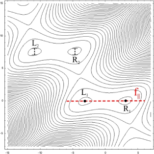
Fig. 2 shows a two-dimensional slice of the potential , after rescaling the capacitance matrix as indicated in Eqs. (3, 4). The slice is chosen to include the two eigendirections of the rescaled curvature matrix of the quadratic part of the potential ( of Eq. 7). In one of these directions the curvature is zero; in this direction only the Josephson energy is nonzero, and the potential is periodic (about two periods are shown in the figure). This periodicity reflects the periodicity of the superconducting phase of the central island of the circuit (the place where , , and meet in Fig. 1). The displacement of the two-dimensional plane shown in Fig. 2 is chosen so that the inductive energy is minimized — recall that the inductive energy consists of a quadratic and a linear part.
The two dots in Fig. 2 indicate the minimum energy points of the potential in this plane, which is almost (but not precisely) the position of the absolute minima (these have also a small component in the other three coordinate directions). We choose the “slow” coordinate of the Born-Oppenheimer approximation to be along the line connecting the two minima in the plane shown; the other four directions are treated as the “fast coordinates”.
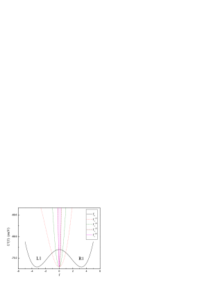
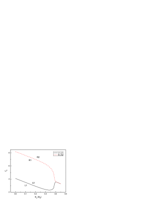
Fig. 3 gives more detail about the potential in these “fast” directions. As expected, the potential rises more steeply in all these directions than in the “slow” direction. The potentials are all basically harmonic, with some noticeable anharmonicity, particularly in the softest “fast” direction . But a calculation of the extent of the ground wavefunction in this direction (error bars near L2 and R2 in Fig. 2) shows that it remains well confined within the harmonic region.
We have chosen a “symmetric” setting for the parameters, , such that the potential is a symmetric double well — the depth of the pair of potential minima in Fig. 2 is equal. This defines a line in the - plane that we refer to as the “S line” (S for symmetric). As the external control parameters and are varied, this potential landscape is changed in two different ways:
-
1.
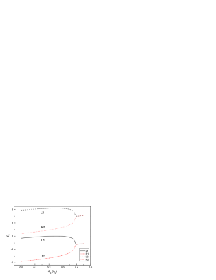
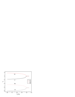
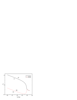
As is varied, the distance between the two minima, and thus the height of the barrier separating them, varies. Increasing from the value shown, , the distance between L1 and R1 (L and R for “left” and ”right”) drops rapidly, as shown by Figs. 6-10, which show how these minimum points evolve as a function of along the S line. As the minima approach one another, the height of the barrier separating the L1 and R1 minima decreases rapidly, as shown in Fig. 11. In this regime the quantum-mechanical tunnel splitting between the lowest-lying energy levels increases dramatically, see Fig. 4. Around the barrier vanishes entirely. There follows a long interval of in which there is only a single minimum per period of the potential; when increases a little beyond , the potential becones quite harmonic around its minimum.
-
2.
As is varied around , the energies of the two minima are shifted with respect to one another. For larger excursions of away from , one minimum becomes unstable, and only one minimum per period remains stable.
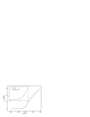
Fig. 5 shows a large region of the - plane, simulating a sequence of measurements very much as they are done in the experiment: For a sequence of values of , is scanned from left to right and back again. Each scan (nearly horizontal line) plots the value of , plus a signal proportional to the classical circulating current in one of the large loops of the qubit. The most prominent feature of this sequence of curves is the thin vertical regions in which the scans are hysteretic. This essentially plots the region in which there is a double minimum in the potential. The shape of this region reflects the behavior of the barrier height with control flux, Fig. 11. Looking at flux , one sees, as one decreases the control flux from about 0.4, a rapid widening of the hysteresis feature, reflecting a rapid increase of the barrier height. The abrupt switch to shrinkage of the hysteresis loop reflects a switching of the lowest barrier from the L1-R1 line to the L1-R2 line. This cuspy feature is readily seen in the experiment Kochnew , and is an excellent landmark for calibrating the actual applied fluxes.
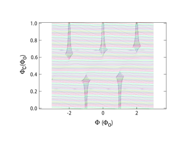
Fig. 5 is clearly periodic with changes in applied flux. Since and are Aharonov-Bohm fluxes (i.e., involving no magnetic field penetrating the interior of the conductors), changing either by an integer multiple of should leave the quantum behavior of the system invariant. This is actually not the periodicity that is seen in Fig. 5. This absence of Aharonov-Bohm periodicity, an apparent violation of gauge invariance, is a result of the fact that the outer perimeter of the qubit is not interrupted by a Josephson junction; because the temperature is very low compared with the superconducting energy gap, there is a very high barrier to the motion of a flux quantum into or out of the device. If this barrier is assumed to be infinite (as it effectively is in our model), the states of the device fall into noncommunicating sectors.
Within these sectors, there remains the periodicity with respect to varying the external fluxes seen in the figure: we can show that if is changed by an integer multiple of , (Each is any integer), the qubit Hamiltonian is invariant if is simultaneously changed by . This shift of and are associated with the phase changes , and . The inductance factors in these expressions are approximate: they are only true in the limit that all mutual inductances are zero. The pattern of invariance as described by these equations is closely matched in experimental data.

The construction of the quadratic and linear parts of the potential in Eq. (7) require a graph-theoretic analysis of the gradiometer circuit, Fig. 1. An appropriate tree for the circuit graph is shown in the inset (b) of Fig. 1. Using this, the loop matrices defined in the Appendix, Eq. (45), can be read off by inspection:
| (21) |
| (22) |
For the numerical analysis of decoherence parameters, we need values for the physical parameters of the circuit. For the C matrix, circuit modeling indicates that we can take it to be a diagonal matrix with diagonal elements (in units of fF). The 10fF capacitances are for the Josephson junctions, the 50fF capacitances are the “strays”. Although the strays are numerically the largest capacitances, they do not affect the results qualitatively, because of their positions in the circuit.
The L matrices are denoted:
| (23) |
| (24) |
| (25) |
The numerical values of these parameters are given in the caption of Fig. 1.
The decoherence parameters involve the temperature, which we take as . This rather high temperature, much larger than the bath temperature of a dilution refrigerator, is an accurate reflection of the effective noise temperature of the circuits coupled to the qubit. Future experiments are planned which will make this effective temperature much lower.
The formal applied flux vector is, . and have been introduced previously, and is the flux in the third loop, the pick up loop. will always to be taken to be zero in the analyses here.
With these matrices we compute the coefficients and using the formulas in the Appendix (Eqs. 69, 70) ( does not occur, as no current sources are present in the circuit). The applied fluxes are time-dependent in the experiments that we are modelling, so in principle we need to retain the full frequency dependence of . The presence of a frequency dependence in this operator is indicative of a retardation phenomenon: the Hamiltonian at time is not a function only of the applied fluxes at time ; rather, because of the lossy elements in the circuit, depends on a convolution of over times preceding . We find, however, that the range in time of the kernel in this convolution is very short: this time range is set by and . For our parameters, this time is no more that 10 psec. In experimentsKochetal , the applied fluxes are varied on a time scale greater than 100psec. For this reason, we ignore this retardation effect in all our calculations here, and set .
IV discussion of and
Figures 12, 13, 14 and 15 show the obtained dissipation and decoherence rates obtained for the gradiometer qubit in the vicinity of the symmetric line, shown as a function of changes in the small- and large-loop bias fluxes ( is taken to be zero throughout). The dependences of these quantities is complex, with variations over a large range of values (note that all the plots are logarithmic). We can explain all the trends seen in these curves. Several key facts determine the overall structure of these curves:
-
•
Many of the curves have a break around , . This is a consequence of a level crossing that occurs near this value of : for larger the lowest two energy eigenvalues of the qubit are both in one energy well. Thus, for the system is too unsymmetrical for the two qubit states to correspond to the left and right wells, and consequently the results in this regime are not of great interest to us.
-
•
For small values of the control flux the barrier is high, and the wave function weight is concentrated near the minima of the two wells. In this regime, which was referred to as the “semiclassical” regime in BKD, the various curves vary in predictable ways as the barrier height and well asymmetry are changed, as we will detail shortly.
-
•
For large values of the control flux the barrier vanishes, and the single remaining well rapidly becomes almost exactly harmonic. It is straightforward to calculate what happens to and in this harmonic limit, and we will see that the data in this regime can be understood with reference to this limit.
-
•
The lossy circuit coupled to the small loop respects the bilateral symmetry of the gradiometer qubit. An exact consequence of this is that and are mathematically symmetric around .
-
•
The lossy circuit coupled to the large loop does not respect the bilateral symmetry of the qubit. Consequently, and are not symmetric, but for several separate reasons (different ones in the semiclassical and harmonic regimes) these functions, for the most part, are very nearly symmetric. Actually, if the Born-Oppenheimer corrections to the decoherence parameters, derived in Sec. II, were left out, would be exactly symmetric.
-
•
The s curves ( and ) are very different from the l curves ( and ). This perhaps surprising result is explained by the fact that the s functions have exactly no contribution from the longitudinal term in the matrix elements (first term in Eq. (II)). The longitudinal term usually dominates the transverse term (second term in Eq. (II)) when it is present, as it is for the l functions. As we will see, this makes the character of these curves very different from one another.
V review of semiclassical analysis
As in BKD, we assume that the potential describes a double well with “left” and “right” minima at
| (26) | |||
| (27) |
Then, the semiclassical approximation amounts to assuming that the left and right single-well ground states and centered at are localized orbitals, having amplitude that vanishes very rapidly away from these minima. Then the two lowest eigenstates can approximately be written as the symmetric and antisymmetric combinations of and ,
| (28) | |||||
| (29) |
where , is the asymmetry of the double well, and is the tunneling amplitude between the two wells. increases almost exponentially with as expected in a WKB picture, see Fig. 4. Since and are localized orbitals, we approximate the matrix elements (see Eq. (II)):
| (30) |
From Eqs. (28)–(30) the eigenstate matrix elements are
| (31) | |||||
| (32) |
where . These formulas will be applied in different ways to explain the four quantities in Figs. 12-15.
In this semiclassical approximation with localized states, the relaxation and decoherence times both diverge if can be made orthogonal to . For a symmetric double well (), for all .
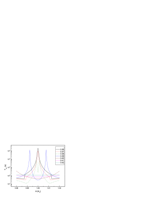
VI
We see in Fig. 12 that as increases, initially is almost constant in and decreasing exponentially with ; this behavior changes fairly abruptly to one which is exponentially increasing in , with a sharp maximum at .
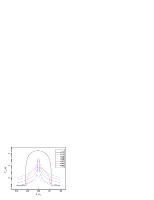
The initial behavior is explained by the semiclassical theory. We must specialize the semiclassical theory to a fact that is special to the circuit coupling to the small loop: as a consequence of the bilateral symmetry of the structure, the “naive” longitudinal contribution to the matrix elements vanishes, i.e.,
| (33) |
With this, we can specialize the matrix element Eq. (31) thus:
| (34) |
We find that, again as a consequence of symmetry, the function has a special form: at the symmetric-well point, it is an even function of (assuming the origin is centered at the midpoint between the two wells); in addition, this symmetry is broken continuously as is made nonzero. This can be summarized by writing the start of the Taylor series for :
| (35) |
Plugging this in and using for gives
| (36) |
| (37) |
This simple functional form fits the curves in Fig. 12 very well for .
For larger the trend of is explained by the observation that around , the barrier disappears and the single minimum rapidly approaches being an ideal harmonic potential. If the potential were exactly harmonic, with its minimum-curvature direction pointed in the direction, then would diverge. The exponential growth of in this regime reflects this approach to harmonicity. At all values of it remains true that for , is divergent, and the lineshapes around reflect this.
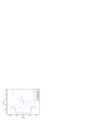
VII
also has two distinct regions, the “semiclassical” and the “harmonic”. In both regions, the longitudinal contributions to the matrix element dominate. This means that symmetry-breaking contributions (for ) remain very small in all regimes (this is untrue for ).
The semiclassical prediction for is
| (38) |
Since is slowly varying with and , we have
| (39) |
This equation predicts a which is exponentially decreasing overall, with a deep minimum at , as seen in the figure.
When the potential becomes harmonic, then should approach a constant almost independent of , since the harmonic oscillator wavefunctions are only shifted by the force proportional to ; the matrix element is independent of this force. is seen to slowly vary with : the variation that is seen presumably reflects the small increase in the harmonic frequency as increases.
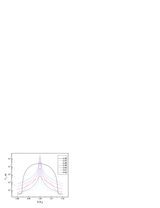
VIII
The semiclassical approximation follows the same development as for , with the result (see (36))
| (40) |
| (41) |
This last equation predicts a strongly diverging with not very much (i.e., ) dependence, as is seen initially in Fig. 14.
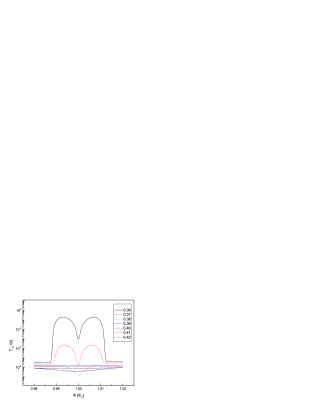
There is a fairly rapid departure from the semiclassical prediction for in that the divergence at splits (symmetrically, as discussed above) into two which rapidly move away from the center. This is explained by the fact that, once the wavefunctions become somewhat delocalized, the difference between the 0 and 1 matrix elements in (40) becomes nonzero, pushing the divergence away from the symmetric point. This difference becomes nonzero because the 0 state (the symmetric state at ) has more amplitude between the two minima than the 1 (antisymmetric) state. Thus, when weighted by the function (recall Eq. (35)), the 0 and 1 matrix elements are (initially) slightly different.
In the harmonic limit, should diverge, just as does. Comparing Figs. 12-14, though, shows that the details of this divergence are rather different. It is evident that as this limit is approached, is dominated by the remaining differences of the 0 and 1 matrix elements just discussed, which become nearly independent as the 0 and 1 wavefunctions become more harmonic.
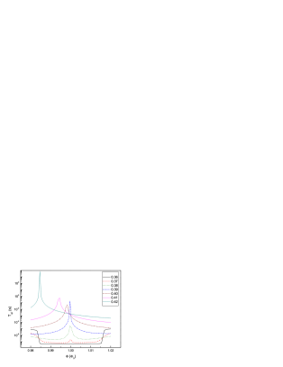
IX
is shown in Fig. 15. In the semiclassical regime this should be
| (42) |
So
| (43) |
For small this predicts, as seen, an almost independent behavior, with a very weak divergence at . As increases, the divergence gets stronger and begins to increase overall.
In the harmonic limit, again, should diverge. But as the contributions disappear, eventually the transverse contributions to the matrix elements begin to be important. These explicitly break the symmetry, as can easily be seen as the shifting of the divergence point in the last few curves.
However, this asymmetry is unlikely to be noticeable experimentally. Recall that the physical and are (approximately BB ) given by summing the and rates. The strong asymmetry in occurs only when its contribution to the rate is very small, and the symmetric will dominate.
X Discussion and Conclusions
We conclude with a discussion of the effect of the presence of stray capacitances, and on the overall implication of our results on decoherence parameters for experiments on the gradiometer qubit.
Figs. 16 and 17 show the results for and for the gradiometer qubit with zero assumed stray capacitances. Graphically, the results are apparently only slightly changed. This is somewhat an impression created by the log scale; a closer examination of the result shows that the presence of stray capacitances actually improves the relaxation time (i.e., makes it longer) by about a factor of 10 in the double-well region, while leaving it more or less unchanged in the harmonic, single-well region.
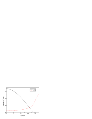
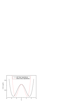
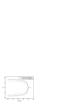
Figs. 18 and 19 provide some explanation for this observation. We see that the double-well potential profile is very similar in the two cases, with the well depths being virtually the same. However, the presence of the strays pushes apart the rescaled distance between the two minima. This diminishes the tunneling between the two wells, and, not surprisingly therefore, lengthens the relaxation time to go from one well to the other. In Fig. 19 we see that this effect persists right up to the point where the two minima merge at around .
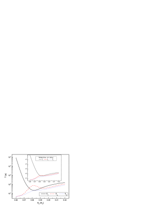
Finally, Fig. 20 gives perhaps the most experimentally relevant summary of our results for the realistic gradiometer qubit parameters (with stray capacitances). During qubit operation, it is envisioned Kochetal that the qubit will be initialized at small control flux, and will then be pulsed rapidly up to high control flux; above , we expect the coherence of the qubit to be protected by an oscillator stabilization not discussed here.
The preferred initialization point is at a value of well below . We see that here we have the right conditions for initialization of the qubit, in that the time will be very long – the figure shows it increasing exponentially as is decreased. This is a simple reflection of the very large barrier height in this region. , and therefore are very small in this region, but this is not harmful during initialization. When is pulsed upwards, quantum dynamics turn on in a region around , where the 0-1 frequency is increasing exponentially through the 100MHz range. This is the relevant frequency because it is roughly the inverse of the anticipated rise time of the pulse in this region, 1-10nsec; this is referred to as the “portal” region in Kochetal .
Thus, the crucial region for the operation of the qubit is in the range of . It is evidently a very perilous region for the qubit: is plunging downward, dropping to around 200nsec, and is increasing from its very small values in the initialization region, but does not rise far beyond 100nsec in this region. Since we expect Kochetal to pulse through this region in under 10nsec, these times are acceptable for qubit operation; but we see that the qubit could not function if it were held in this region of without any other protective mechanism for a long time. Also, we must beware of other effects, such as higher effective temperatures or stronger mutual inductance couplings, that would make these times even worse. We believe that there have been occasions when the conditions of the experiment were worse by a factor of 10 or more; in this case, the qubit’s coherence is not likely to survive even a 10nsec traversal of this region of parameter space.
Fig. 20 is obtained by adding the inverse relation times arising from the small-loop and large-loop circuits (we ignore the small nonadditive effects explored in BB ). is, though the whole region of interest, dominated by . For small , is also dominated by the large-loop circuit; however, for the small-loop dephasing becomes dominant. So, we see that the analysis of both circuits is experimentally relevant.
Finally, the inset to Fig. 20 shows the effects of imperfections in the setting of , which would put the system off the S line. We see that, even for departures of , there are noticeable changes in the decoherence parameters. is actually increased, reflecting the fact that has a minimum at the S line. But the system’s sensitivity to phase fluctuations increases – is smaller off the S line. While the changes seen from the S line are not dramatic, these results indicate that much larger departures should be treated with caution, and subject to a full analysis.
A concluding word: The results reported here have been a useful guide to experiment, but they have shown their greatest worth when they are part of the iterative design process itself. Thus, even the rather complete snapshot given here does not do justice to the full role that this analysis has had in the process of perfecting the gradiometer qubit. The work has already passed on to further questions not touched on here, such as the role of additional harmonic oscillator circuits in modifying the decoherence parameters Kochetal ; Kochnew , and the problems created by introducing qubit-qubit coupling. An intimate relationship between theory and experiment will continue to be crucial in the continuing development of this qubit technology.
Acknowledgments
DPDV is supported in part by the NSA and ARDA through ARO contract number W911NF-04-C-0098. FB is supported by Fundação de Amparo à Pesquisa do Estado de São Paulo (FAPESP). RHK thanks the support of DARPA under contract MDA972-01-C-0052.
Appendix: Circuit Theory
We make extensive use here of the systematic analysis of flux qubits initiated in BKD. For completeness, we review the formalism presented there, both the network graph theory and the Caldeira-Leggett analysis. We have added some extensions to this theory, which we separate out and present in a separate subsection of this appendix.
X.1 Review of BKD
This subsection is a streamlined summary of the results presented in BKD .
An oriented graph consists of nodes and branches . In circuit analysis, a branch represents a two-terminal element (resistor, capacitor, inductor, current or voltage source, etc.), connecting its beginning node to its ending node . A loop in is a connected subgraph of in which all nodes have degree two (the degree of a node is the number of branches containing ). For each connected subgraph we choose a tree , i.e. a connected subgraph of which contains all its nodes and has no loops. The branches that do not belong to the tree are called chords. The fundamental loops of a subgraph are defined as the set of loops in which contain exactly one chord .
A complete description of the topology of the network is provided by the fundamental loop matrix, defined as
| (44) |
where and . By labeling the branches of the graph such that the first branches belong to the tree , where is the number of disjoint connected subgraphs of , we obtain
| (45) |
where , the loop matrix, is an matrix.
The state of an electric circuit described by a network graph can be defined by the branch currents , where denotes the electric current flowing in branch , and the branch voltages , where denotes the voltage drop across the branch . If we divide the branch currents and voltages into a tree and a chord part,
| (46) | |||||
| (47) |
Then the Kirchhoff laws can be stated very succinctly and universally:
| (48) | |||||
| (49) |
Here are the external magnetic fluxes threading the loops.
To write the Hamiltonian of the electrical circuit, we must further distinguish the different types of electrical circuit elements in the graph. We write
| (52) |
The sub-matrices will be called loop sub-matrices. The different chord labels are for Josephson junctions (J), linear inductors (L), shunt resistors (R) and other external impedances (Z), and bias current sources (B). Without loss of generality the capacitors (C) can all be taken as tree branches. The tree inductors are labeled (K). We note here that in our formalism all capacitors should be considered to be in parallel with a Josephson junction, even if it is one with zero critical current.
Finally, to fully define the problem, the electrical characteristics of each branch type should be defined. The current-voltage relations for the various types of branches are
| (53) | |||||
| (54) | |||||
| (55) | |||||
| (56) | |||||
| (63) |
Here the diagonal matrix contains the critical currents of the junctions on its diagonal, and is the vector . Eq. (54) describes the (linear) capacitors ( is the capacitance matrix), and the junction shunt resistors are described by Eq. (55) where is the (diagonal and real) shunt resistance matrix. The external impedances are described by the relation Eq. (56) between the Fourier transforms of the current and voltage, where is the impedance matrix. The external impedances can also defined in the time domain,
| (64) |
where the convolution is defined as
| (65) |
Causality allows the response function to be nonzero only for positive times, for . In frequency space, the replacement with guarantees convergence of the Fourier transform 111We choose the Fourier transform such that it yields the impedance for an inductor (inductance ).
| (66) |
In our formalism it is necessary to distinguish chord from tree inductors, so the inductance matrix must be written in block form shown in Eq. (63).
With all these definitions, a universal equation of motion for the electric circuit reads
| (67) |
This equation as presented is a slight extension of BKD, in that and are allowed to be time dependent. If they are time independent, then the expressions for the coefficients of this equation of motion are:
The coefficients of this equation are as follows
| (68) |
| (69) |
| (70) |
| (71) |
| (72) |
| (73) |
With the definitions, as given in BKD :
| (74) |
| (75) |
| (76) |
| (77) |
| (78) |
| (79) |
| (80) |
| (81) |
| (82) |
| (83) |
| (84) |
| (85) |
The last two terms of Eq. (67) describe dissipation, handled by the Caldeira-Leggett (see CG ), to be reviewed shortly. The remaining terms are generated by a (time dependent) system Hamiltonian:
| (86) |
| (87) | |||||
Performing a standard Born-Markov approximation for the system dynamics, one obtains predictions for the relaxation times of the system:
| (88) | |||||
| (89) |
We consider the external impedances contributing to decoherence one at a time (for an analysis of non-additive effects, see BB ). , which determines the quantities in Eq. (88, 89), then has the form,
| (90) | |||||
| (91) | |||||
| (92) | |||||
| (93) |
where is a scalar real function, is the normalized vector parallel to , and is the length of the vector ( is the eigenvalue of the rank 1 matrix ). Also
| (94) |
X.2 New results
The following expressions were not contained in BKD, and are new to this paper.
The full frequency dependent expressions for and are:
| (95) |
| (96) |
In our previous work we assumed that and were time independent, so that only the limit of these expressions were presented.
A final result: it is amusing the write out the full expression for , from which is easily constructed, in terms of the basic input matrices (loop matrices F and inductance matrices L):
It is clear why it is more manageable to write this expression in terms of intermediate quantities; one can see that it involves up to four nested inverses.
References
- (1) G. Burkard, D. P. DiVincenzo, P. Bertet, I. Chiorescu, and J. E. Mooij, “Asymmetry and decoherence in a double-layer persistent-current qubit”, cond-mat/0405273, Phys. Rev. B 71, 134504 (2005).
- (2) P. Bertet, I. Chiorescu, G. Burkard, K. Semba, C. J. P. M. Harmans, D. P. DiVincenzo, and J. E. Mooij, “Relaxation and Dephasing in a Flux-qubit,” cond-mat/0412485, submitted to Phys. Rev. Lett.
- (3) Y. Nakamura, Yu. A. Pashkin, and J. S. Tsai, “Coherent control of macroscopic quantum states in a single-Cooper-pair box”, Nature 398, 786 (1999).
- (4) Y. Makhlin, G. Schön, and A. Shnirman, “Quantum-state engineering with Josephson-junction devices”, Rev. Mod. Phys. 73, 357 (2001).
- (5) R. H. Koch, J. R. Rosen, G. A. Keefe, F. M. Milliken, C. C. Tsuei, J. R. Kirtley, and D. P. DiVincenzo, “Low-bandwidth control scheme for an oscillator-stabilized Josephson qubit,” Phys. Rev. B, 72, 092512 (2005).
- (6) G. Burkard, R. H. Koch, and D. P. DiVincenzo, Phys. Rev. B 69, 064503 (2004).
- (7) A. O. Caldeira and A. J. Leggett, “Quantum tunnelling in a dissipative system”, Annals of Physics 149, 374 (1983), and “Influence of damping on quantum interference: An exactly soluble model”, Phys. Rev. A 31, 1059 (1985).
- (8) E. Mertzbacher, Quantum Mechanics (2nd Edition, Wiley, New York, 1970).
- (9) G. Burkard and F. Brito, “Nonadditivity of decoherence rates in superconducting qubits”, Phys. Rev. B 72, 054528 (2005).
- (10) R. H. Koch, J. R. Rosen, G. A. Keefe, F. M. Milliken, C. C. Tsuei, J. R. Kirtley, and D. P. DiVincenzo, “Experimental demonstration of an oscillator-stabilized Josephson qubit,” submitted to Phys. Rev. Lett.