Longitudinal and spin-Hall conductance
of a two-dimensional Rashba system with arbitrary disorder

Abstract

We calculate the longitudinal and spin-Hall conductances in four-lead bridges with Rashba - Dresselhaus spin-orbit interactions. Numerical results are obtained both within Landauer-Büttiker formalism and by the direct evaluation of the Kubo formula. The microscopic Hamiltonian is obtained in the tight-binding approximation in terms of the neareast-neighbor hopping integral $t$, the Rashba spin-orbit coupling $V_{R}$, the Dresselhaus spin-orbit coupling $V_{D}$ and an Anderson-like, on-site disorder energy strength $W$. We reconfirm that below a critical disorder threshold, the spin-Hall effect is present. Further, we study the effect on the two conductivities of the Fermi energy, Rashba/Dresselhaus coefficient ratio, and system size.

I Introduction

Known to exist for a long time general , the spin-orbit (SO) coupling in two dimensional electronic systems (2DEG) has received a lot of attention lately motivated by its potential applications in spintronics. Recent experimentsSdH have demonstrated that the magnitude of the spin-orbit coupling can be modified by a voltage gate, hence generating the premise of the possible manipulation of spin currents by electric fields alone. The two sources of the spin-orbit coupling are the inversion asymmetry of the confining potential in the direction perpendicular to the 2DEG (Rashba) and the bulk asymmetry and interface inversion asymmetry (Dresselhaus)Dresselhaus .

In a very interesting developmentSinova , Sinova et. al predicted that a spin-Hall current of transverse spin component appears in a 2DEG with SO coupling as a response to a in-plane electric field. This spin current has a universal value, equal to $e/8\pi$. The intrinsic spin-Hall effect is quite different from the extrinsic spin-Hall effectHirsch proposed by Hirsch, which is generated by impurity scattering. The possible existence and persistence in disordered systems of the intrinsic spin-Hall effect (SHE) have been the focus of many recent papersrecent . The question of whether arbitrary small amounts of disorder suppress or not the intrinsic SHE is still awaiting a definite answer. Some analytical calculations Zhang claim that SHE does not survive even in the weak disorder regime, while others Murakami provide arguments that SHE is robust and weak disorder in the system is not enough to destroy this effect. While the problem was studied in more detailed using analytical methods, there are few unbiased numerical calculationsNikolic at present.

In this work, we present numerical results for the longitudinal and spin-Hall conductivities of a 2DEG with spin-orbit interactions, both Rashba and Dresselhaus, in the presence of disorder. These values are obtained within a spin-dependent Landauer-Buttiker formalism, developed for a microscopic Hamiltonian written in a tight-binding approximation that incorporates both the spin-orbit interaction and disorder. As a further check, we calculate the same conductances by using the Kubo formalism and find good agreement between the two sets of results. Our findings suggest that the spin-Hall effect occurs in disordered systems, for as long as the disorder remains below a critical threshold value. We also study the dependence of the conductivities on the Fermi energy, system size, and on the relative strengths of the two types of SO coupling.

In the section II of the paper we present the general framework of spin-dependent LB formalism used for computing the spin-Hall conductance, while in section III we show and discuss our results. For comparison, in the appendix, we compute the same conductances by using the Kubo formalism.

II System Description

The single particle Hamiltonian for an electron of momentum $\mathbf{p}=(p_{x},p_{y})$, spin $\boldsymbol{\sigma}=(\sigma_{x},\sigma_{y},\sigma_{z})$, and effective mass $m^{*}$, in a 2DEG with Rashba ($\alpha$) and Dresselhaus ($\beta$) spin-orbit interactions is:

$$H=\frac{{\mathbf{p}}^{2}}{2m^{\star}}+\alpha\left(\sigma_{x}p_{y}-\sigma_{y}p_{x}\right)+\beta\left(\sigma_{x}p_{x}-\sigma_{y}p_{y}\right)\;.$$ (1)

The relative strengths of the Rashba and Dresselhaus terms, $\alpha/\beta$ describing the spin-orbit coupling in semiconductor quantum wells, are available from photocurrent measurementsGanichev . The interplay of the two SO couplings has been also lately subject to intense theoretical investigations with respect to other physical phenomena such as magneto-oscillation phenomena in quantum wells or spin splitting of the electron energy states in quantum dots rashba_dressel .

We discretize the Hamiltonian using a tight-binding approach, where the solution domain is filled with a regular virtual lattice. The Hamiltonian is constructed over this lattice assuming only neareast-neighbor coupling. This can be done straightforwardly by using the projections on $x$ and $y$ direction of the momentum operator ${\mathbf{p}}=-i\hbar\nabla$ in Eq. (1). The resulting tight-binding Hamiltonian is:

$$H = \sum\limits_{i,\alpha,}\varepsilon_{i}c_{i\alpha}^{\dagger}c_{i\alpha}-t\sum\limits_{<i,j>,\alpha}c_{i\alpha}^{\dagger}c_{j\alpha}$$

$$+ V_{R}\sum\limits_{i}\left[\left(c_{i\uparrow}^{\dagger}c_{i+\delta_{x}\downarrow}-c_{i\downarrow}^{\dagger}c_{i+\delta_{x}\uparrow}\right)\right.$$

$$-i\left.\left(c_{i\uparrow}^{\dagger}c_{i+\delta_{y}\downarrow}+c_{i\downarrow}^{\dagger}c_{i+\delta_{y}\uparrow}\right)\right]$$

$$+ V_{D}\sum\limits_{i}\left[(-i)\left(c_{i\uparrow}^{\dagger}c_{i+\delta_{x}\downarrow}+c_{i\downarrow}^{\dagger}c_{i+\delta_{x}\uparrow}\right)\right.$$

$$+\left.\left(c_{i\uparrow}^{\dagger}c_{i+\delta_{y}\downarrow}-c_{i\downarrow}^{\dagger}c_{i+\delta_{y}\uparrow}\right)\right]\;.$$

Here $t=\hbar^{2}/(2m^{\star}a_{0}^{2})$ is the hopping integral, $V_{R}=\hbar\alpha/a_{0}$ and $V_{D}=\hbar\beta/a_{0}$ are the Rashba and Dresselhaus coupling strengths, respectively, renormalized by the lattice constant $a_{0}$, and $\delta_{x}$ and $\delta_{y}$ are the unit vectors along the $x$ and $y$ directions. The hopping matrix element $t$ represents the unit of energy in our calculations. The second, third, and last terms in Eq. (II), can be combined and a compact expression for the Hamiltonian can be written in the form:

$$H = \sum\limits_{i,\mu}\varepsilon_{i}c_{i\mu}^{\dagger}c_{i\mu}-\sum\limits_{<i,j>,\mu,\nu}t_{ij}^{\mu\nu}c_{i\mu}^{\dagger}c_{j\nu}\;,$$ (3)

where $c_{j\mu}$ $(c_{j\mu}^{\dagger})$ is the annihilation (creation) operator of an electron of spin index $\mu$ at site $j$. The first term in Eq. (3) is the on-site disorder, as in the Anderson model, with $\varepsilon_{i}$, a random energy generated by a box distribution $\varepsilon_{i}\in[-W/2,W/2]$. The SO interactions are directly incorporated in the hopping term which acquires position and spin dependence.

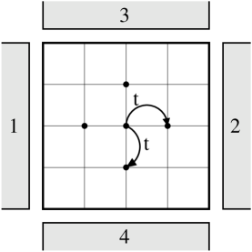
Figure 1: Graphical depiction of the lattice model used for computing the spin-Hall conductance. Four metallic leads (represented as the dashed regions) acting as injector (1), detector (2) and voltage probes (3 and 4) are are attached to the 2DEG. Position and spin dependence are not explicitly decided for the hopping integral.

The Hamiltonian given by Eq. (3) is studied in a N$\times$N square lattice, as presented in Figure 1. Each metallic lead attached to the sample is considered a perfect semi-infinite wire, without disorder and SO interactions. $V_{R}$ and $V_{D}$ are also assumed to be zero in leads 3 and 4 in order to avoid spin flips at the boundaries. Throughout our calculations we use the same values for the cross sections of leads and sample, in order to eliminate scattering induced by the wide-to-narrow geometry Szafer .

Within the LB formalism the total current in terminal $p$ is given by $I_{p}=e^{2}/h\sum_{q\neq p}T_{pq}(V_{p}-V_{q})$ where the sum is over all the other leads $q$ connected to the system. Spin current can be defined in a similar way, up to a constant: $I_{p,\mu}^{spin}=e/(4\pi)\sum_{q\neq p,\nu}T_{pq}^{\mu\nu}(V_{p}-V_{q})$. The voltages are computed by considering ballistic transport between all the connected terminals and imposing the following boundary conditions: $V_{2}=0$ (fixes the arbitrary zero of voltage), $I_{3}=2e/\hbar\sum_{\alpha}I_{3,\alpha}^{spin}=0$, $I_{4}=2e/\hbar\sum_{\alpha}I_{4,\alpha}^{spin}=0$ (terminals $3$ and $4$ are voltage probes) and $I_{1}+I_{2}=0$, (guarantees that current flows between terminals $1$ and $2$). The zero temperature conductance, $\mathbf{G}$, that describes the spin-resolved transport measurements, is related with the transmission matrix $\mathbf{T}$, as in :

$${\mathbf{G}}=\frac{e^{2}}{h}{\mathbf{T}}=\frac{e^{2}}{h}\left(\begin{array}[]{cc}T^{\uparrow\uparrow}&T^{\uparrow\downarrow}\\ T^{\downarrow\uparrow}&T^{\downarrow\downarrow}\end{array}\right),$$ (4)

[Indices $p$ and $q$ were suppressed in writing Eq. (4)]. $T_{pq}^{\mu\nu}$ represents the transmission probability over all the conduction channels to detect a spin $\mu$ in the lead $p$ arising from an injected spin $\nu$ electron in lead $q$, when both spin-flip and non-spin-flip processes are considered. The transmission coefficient can be calculated as $T_{pq}^{\mu\nu}=Tr[\Gamma_{p}^{\mu}G_{R}\Gamma_{q}^{\nu}G_{A}]$ where $\Gamma_{p}^{\mu}=i(\Sigma_{p}^{\mu}-\Sigma_{p}^{\mu\dagger})$ with $\Sigma_{p}^{\mu}$ the retarded self-energy due to the interaction between the sample and the lead for spin-channel $\mu$. The self-energy contribution is computed by modeling each terminal as a semi-infinite perfect wire. In our tight-binding model, the hopping between the lead orbitals and between the leads and the sample orbitals are equalDatta with $t$ (unit of energy). The self-energy matrix, which is diagonal in spin indices, can be written as:

$$\Sigma_{p}=\left(\begin{array}[]{cc}\Sigma_{p}^{\uparrow}&0\\ 0&\Sigma_{p}^{\downarrow}\end{array}\right)$$ (5)

with $\Sigma_{p}^{\uparrow}=\Sigma_{p}^{\downarrow}$ for a perfect metallic lead. The retarded Green’s function is computed as $G_{R}=(E_{F}-H-\sum_{p=1}^{4}\Sigma_{p})^{-1}$, where $E_{F}$ is the Fermi energy and $H$ is the Hamiltonian in Eq. (3). The advanced Green’s function is, of course, $G_{A}=G_{R}^{\dagger}$.

In the LB formalism, the total scattering between two lead $p$ and $q$ can be simply written as the sum over all spin components $T_{pq}=T_{pq}^{\uparrow\uparrow}+T_{pq}^{\uparrow\downarrow}+T_{pq}^{\downarrow\uparrow}+T_{pq}^{\downarrow\downarrow}$. Two other useful combinationsSouma are $T_{pq}^{in}=T_{pq}^{\uparrow\uparrow}+T_{pq}^{\uparrow\downarrow}-T_{pq}^{\downarrow\uparrow}-T_{pq}^{\downarrow\downarrow}$ and $T_{pq}^{out}=T_{pq}^{\uparrow\uparrow}+T_{pq}^{\downarrow\uparrow}-T_{pq}^{\uparrow\downarrow}-T_{pq}^{\downarrow\downarrow}$. $T_{pq}^{out}$ represents the difference between the transmission probabilities to detect an electron in the lead $p$ arising from an injected spin $\uparrow$ ($\downarrow$) electron in lead $q$. These expressions allow us to compute the spin-Hall conductance, as

$$G_{sH}=\frac{I_{3,\uparrow}^{spin}-I_{3,\downarrow}^{spin}}{V_{1}}$$ (6)

Finally, by using the voltages obtained inverting the multiprobe equations, the spin-Hall conductance becomes:

$$G_{sH}=e/(8\pi)(T_{13}^{out}+T_{43}^{out}+T_{23}^{out}-T_{34}^{in}-2T_{31}^{in})\;.$$ (7)

At the same time, the longitudinal conductance, $G_{L}=I_{2}/(V_{1}-V_{2})$, is written as:

$$G_{L}=e^{2}/h\left(T_{21}+0.5\,T_{32}+0.5\,T_{42}\right)\;,$$ (8)

when four terminals are connected to the sample as in Figure 1. The spin-Hall and longitudinal conductances are the central quantities of our analysis. In the next section, we present results showing their dependence on the Fermi energy, system size, and disorder strength.

III Results and Discussion

Clean limit. The clean limit dependence of the spin-Hall conductance (SHC) on the Fermi energy is shown in Figure 2. The electron-hole symmetry is preserved throughout the calculation, so the SHC vanishes at the band center $E_{F}=0$ and is an odd-function relative to the Fermi energy, in agreement with the results of Ref [Nikolic, ]. The small oscillations observed in the energy dependence are finite size effects related with the discontinuities in the self-energy contribution from the terminals and with the discrete energy levels.

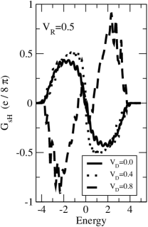
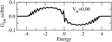
Figure 2: Upper left panel: The Fermi energy dependence of the spin-Hall conductance (SHC) of a two dimensional four-probe bridge in the clean limit, for a fixed Rashba coupling $V_{R}=0.5$ and for different Dresselhauss energies. Upper right panel: SHC dependence on $V_{D}$ for different Rashba couplings, for Fermi energy $E_{F}=-2t$ in the clean limit. For $V_{R}=V_{D}$, the SHC vanishes. The system size is $20\times 20$. Lower panel: The SHC represented as function of $E_{F}$ for $V_{R}=0.06$ and $V_{D}=0.0$.

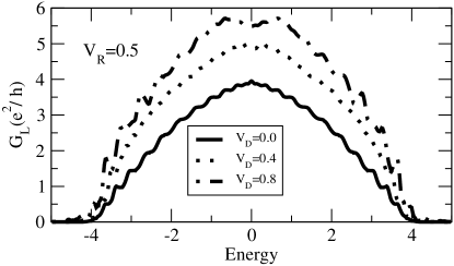
Figure 3: The longitudinal conductance as function of the Fermi energy for different Dresselhaus SO couplings, as indicated. The system size is $20\times 20$.

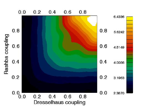
Figure 4: (Color online) Longitudinal conductance plotted as a function of $V_{R}$ and $V_{D}$ for a system size $20\times 20$ and for a Fermi energy $E_{F}=-2t$. The spectrum is anti-symmetric along the $V_{D}=V_{R}$ line. The spin-Hall conductance is positive for $V_{R}>V_{D}$, negative for $V_{R}<V_{D}$ and vanishes for $V_{D}=V_{R}$.

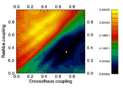
Figure 5: (Color online) The spin-Hall conductance plotted as a function of $V_{R}$ and $V_{D}$ for a system size $20\times 20$ and for a Fermi energy $E_{F}=-2t$. The spectrum is anti-symmetric along the $V_{D}=V_{R}$ line. The spin-Hall conductance is positive for $V_{R}>V_{D}$, negative for $V_{R}<V_{D}$ and vanishes for $V_{D}=V_{R}$.

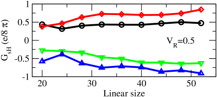
Figure 6: (Color online) Linear system size dependence of the spin-Hall conductance for a Fermi energy $E_{F}=2.0t$, with $V_{R}=0.5$ and for $V_{D}$ = {0.0 $(\circ)$, 0.3 $(\diamond)$, 0.6 $(\bigtriangledown)$, and 0.9 $(\bigtriangleup)$}.

Another important parameter is the ratio $r=V_{R}/V_{D}$. When $r=1$, for any energy, $G_{sH}=0$ (see Fig. 2 - right panel, and Fig. 5). For a hole-like behavior ($E_{F}<0$) and $r>1$, $G_{sH}$ is positive, while for $r<1$, $G_{sH}$ changes sign, demonstrating that the spin current is generated in the direction of the major driving field Sinitsyn . ExperimentallyGanichev ; Knap , the tuning parameter $r$ could be varied between $1.5$ and $2.5$.

Figure 3 presents the effect of the Dresselhaus SO coupling on the longitudinal conductance as function of Fermi energy, for a fixed value of the Rashba coupling. In contrast, in Fig. 4 the Fermi energy is fixed to $E_{F}=-2t$ and the longitudinal conductance is plotted as function of both Rashba and Dresselhaus interactions. Here, $r=1$ still represents a symmetry line in the parameter space ($V_{R},V_{D}$). For a fixed value of the Fermi energy, we found the symmetry relation: $G_{L}(V_{R},V_{D})=G_{L}(V_{D},V_{R})$.

In Figure 5 we present the spin-Hall conductance as function of $V_{R}$ and $V_{D}$. SHC is anti-symmetric along the $V_{D}=V_{R}$ line. The Fermi energy is fixed at $E_{F}=-2t$ and the system size is $20\times 20$. For a lattice parameter of $a_{0}=5.0$ nm and electron effective mass $m^{\star}=0.068m$ (in GaAs), the hopping integral is $t\simeq 19.0$meV. A typical value for the Rashba couplingMiller is $\sim 50-80$ meV$\cdot$Å, which corresponds to $V_{R}=1-1.6$ meV, with a typical ration $V_{R}/t\simeq 0.05-0.08$. The results presented in Fig. 2 (upper panel) are beyond the experimental reach. In Figure 2 (lower panel) we represent the Fermi energy dependence of the SHC with a experimental accessible value for the spin-orbit interaction strength, and, as expected, the SHC amplitude is strongly reduced. However, the overall behavior is preserved.

The effect of scaling as function of system size is presented in Figure  6. Spin Hall conductance is essentially constant up to, at least, system sizes $50\times 50$. However we emphasize that the effect of boundaries, due to the attached leads, may be very important and in principle can hide the true nature of the bulk spin-Hall effect.

Our analysis shows that in the clean limit, a non-universal value for SHC exists, in agreement with other numerical calculationsNikolic . SHC strongly depends on the strength of spin-orbit couplings, while the spin current is always along the driving field in the system and depends on the relative strength of the Rashba and Dresselhaus couplings. In the hole-like (electron-like) regime, characterized by $E_{F}<0$ ($E_{F}>0$), $sgn(SHC)\sim\pm sgn(V_{R}-V_{D})$.

Arbitrary disorder. A system with time reversal symmetry, but with spin rotational symmetry broken by the spin-orbit coupling, belongs to the symplectic universality class. It is well established by now that $SU(2)$ models with chiral symmetry exhibit an Anderson transition in two-dimensionOhtsuki . Critical disorder strength was estimated to be $W_{C}\simeq 5.9$ and the critical exponent for the localization length $\nu\simeq 2.74$. In our model, different values for the hopping coupling may lead to different values for the disorder strength. However, it is understood that SHC cannot survive in the insulating regime of a 2DEG, because any localized state cannot contribute to SHC. It is still not clear whether SHC vanishes in the diffusive transport when the mobility edge $\pm E_{C}$ moves towards the band center and localized states in the band tails coexist with extended states in the band center. To answer this question we study the effect of disorder on SHC. In Figure 7 (Left panel) we represent the SHC as function of disorder strength for different $V_{D}$. We find that $G_{sH}$ can be suppressed by a strong scattering when $W\geq 4-5$, close to the metal-insulator transition disorder strength. In the left panel the Dresselhaus coupling is zero and the Rashba coupling strength dependence of SHC is presented. For comparison we have plotted also the result when no disorder is present in the system.

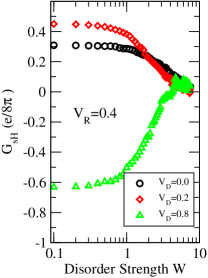
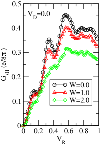
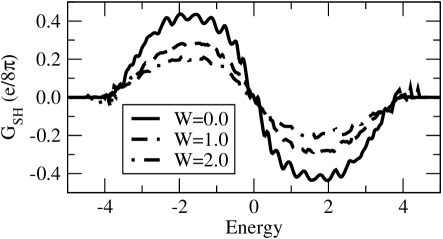
Figure 7: (Color online) Left: Disorder strength dependence of the SHC with Rashba spin-orbit strength $V_{R}=0.4$. Right: SHC as function of Rashba coupling for different disorder strengths $W$. Lower panel: SHC as function of Fermi energy and for different disorder strengths $W$. Electron-hole symmetry is preserved in the presence of disorder. In the upper panel Fermi energy is $E_{F}=-2.0t$. System size is $16\times 16$ in all figures.

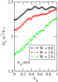
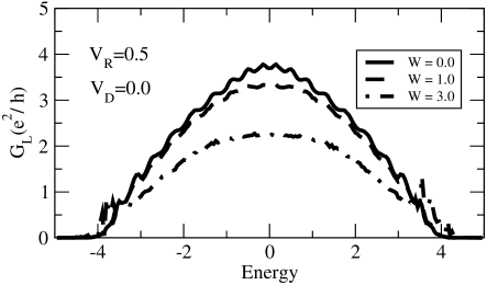
Figure 8: (Color online) Longitudinal conductance as function of disorder strength (upper left panel), and as function of Rashba spin-orbit coupling strength (upper right panel) for different disorder amplitude. Lower panel: Effect of disorder on the energy dependence of the longitudinal conductance. The system size is $16\times 16$. Disorder average is over 1000 samples.

Energy dependence was also considered in the presence of disorder. (see Figure 7, lower panel).

In the insulating regime, all states are localized, so the absence of extended states available for transport at the Fermi level leads to a vanishing SHC. When disorder is weak enough, extended states in the band center coexist with insulating states localized mostly in the band tails. These extended states may be responsible for non-vanishing SHC when small amounts of disorder are present in the system.

It is well known that in Landauer-Büttiker formalism the attached leads play an important role, affecting the system self-energy, and can alter the nature of the bulk spin-Hall effect, while this is not the case in the Kubo formalism.

To study the effect of terminals on the spin-Hall and longitudinal conductances we did a direct calculation of conductances within the Kubo formalism (see the appendix for further details). We found good agreement between the conductance values obtained in both the LB and Kubo formalisms. In Figure  9 we present the these results for a system of size $16\times 16$. The electron-hole symmetry is also preserved in the Kubo formalism, so the spin-Hall conductance vanishes at half filling, as in the LB formalism.

In Ref. Sinitsyn, , Sinitsyn et. al. and Shen use the Kubo formula to compute the spin-Hall conductance analytically, when both the Rashba and Dresselhaus couplings are considered. As in our case, they find that the spin-Hall conductance vanishes when the Rashba and Dresselhaus couplings have the same strength. The predicted value of the SHC, however, is a constant $\pm e/8\pi$, depending on the ration $V_{R}/V_{D}$. In contrast, in our numerical approach, the SHC is no longer a universal constant, but rather a function of the Fermi energy and of the Rashba/Dresselhaus coupling strengths.

IV Conclusions

In this work we have investigated the longitudinal and spin-Hall conductances of a two dimensional electronic system with Rashba and Dresselhaus spin-orbit coupling in the framework of a tight binding approximation. For the main part of the work we have used Landauer-Büttiker formalism combined with Green’s function approach to study the efect of spin-orbit coupling and disorder on $G_{L}$ and $G_{sH}$. Our results for the spin Hall conductance, as function of Fermi energy and disorder strength, in the case when Dresselhaus coupling is neglected, agree with the results of Ref. Nikolic, which is a special case of the present model.

We have also computed the Fermi energy dependence of longitudinal and spin-Hall conductances in the Kubo formalism. The good agreement found between the two sets of conductances computed in LB and Kubo formalisms strengthens the assumption that the spin-Hall effect is a bulk property of the system. However, further studies are needed in order to clarify the role of terminals. For example, one can investigate the scaling of spin-Hall conductance as function of the system size, both in the Landauer-Büttiker and the Kubo formalisms.

Appendix A Comparison with the Kubo formalism

In this Appendix we present the derivation for the Kubo formula used for computing the longitudinal and spin-Hall conductances.

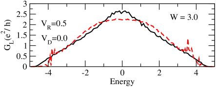
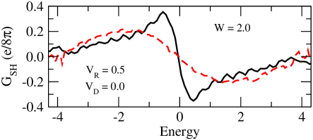
Figure 9: (Color online) Longitudinal (upper panel) and spin-Hall conductance (lower panel) for a system size of $16\times 16$. Solid lines represent results obtained using Kubo formalism while the dashed lines are obtained using Landauer-Büttiker method. Results are average over 500 samples. Energy is measured in units of $t$.

In terms of single particle states, the longitudinal conductivity can be computed from the general Kubo formula:

$$\sigma_{L}\left({\mathbf{r}},{\mathbf{r}}^{\prime}\right)=-i\,\hbar\sum_{n,n^{\prime}}\frac{P_{n^{\prime}}-P_{n}}{E_{n^{\prime}}-E_{n}}\frac{\left<n^{\prime}\left|{j_{x}}({\mathbf{r}})\right|n\right>\left<n\left|{v_{x}}({\mathbf{r}}^{\prime})\right|n^{\prime}\right>}{E_{n^{\prime}}-E_{n}+i\,\hbar 0^{+}}.$$ (9)

Similarly, for the spin-Hall conductance we write:

$$\sigma_{sH}\left({\mathbf{r}},{\mathbf{r}}^{\prime}\right)=\sum_{n,n^{\prime}}\frac{P_{n^{\prime}}-P_{n}}{E_{n^{\prime}}-E_{n}}\frac{Im\left<n^{\prime}\left|j_{x}^{z}({\mathbf{r}})\right|n\right>\left<n\left|v_{y}({\mathbf{r}}^{\prime})\right|n^{\prime}\right>}{E_{n^{\prime}}-E_{n}+i\,\hbar 0^{+}}.$$ (10)

The single-particle states are constructed from the site orbitals as $b_{n}^{\dagger}=\sum_{i,\alpha}\psi_{n}\left(i,\alpha\right)c_{i\alpha}^{\dagger}$. Operator $b_{n}^{\dagger}$ stands for the creation of a single particle state $\left|n\right>$ from the one-electron wave functions, $\psi_{n}\left(i,\alpha\right)$. The wave functions $\psi_{n}\left(i,\alpha\right)$ and the corresponding eigen-energies $E_{n}$ can be easily obtained by solving the eigen-value problem for the Hamiltonian (3).

The velocity operator is defined by the commutator: $i\,\hbar{\mathbf{v}}=\left[{\mathbf{r}},H\right]$, while the spin current is given in terms of the anticommutator between the velocity operator and Pauli matrix $\sigma_{z}$: $j_{x}^{z}=\hbar/4\left\{\sigma_{z},v_{x}\right\}$. A simple quantum mechanics calculation gives for the current and for the spin-current operators the following expressions:

$$\left<n\left|{\mathbf{v}}\right|n^{\prime}\right>=\frac{1}{i\,\hbar}\sum_{i,j,\alpha,\beta}\psi_{n}^{*}\left(i,\alpha\right)\left[\left({\mathbf{r}}_{i}-{\mathbf{r}}_{j}\right)H_{ij}^{\alpha,\beta}\right]\psi_{n}\left(j,\beta\right)$$ (11)

$$\left<n\left|{\mathbf{j}}^{z}\right|n^{\prime}\right>=\frac{e}{4\,i}\sum_{i,j,\alpha,\beta}\psi_{n}^{*}\left(i,\alpha\right)\left[\left({\mathbf{r}}_{i}-{\mathbf{r}}_{j}\right)\tilde{H}_{ij}^{\alpha,\beta}\right]\psi_{n}\left(j,\beta\right).$$ (12)

In Eq. (12), $\tilde{H}=\left\{\sigma_{z}\otimes{\mathbf{1}},H\right\}$.

At $T=0K$, when the Fermi function derivative is approximated by a delta function, we write:

$$\frac{P_{n^{\prime}}-P_{n}}{E_{n^{\prime}}-E_{n}} = \int dE\,\frac{\partial f(E)}{\partial E}\,\delta(E_{n}-E)$$ (13)

$$= -\delta(E_{n}-E_{F}).$$

Incorporating Eqs. (11), (12), (13) in Eqs. (9) and (10) a simple expression for longitudinal and spin-Hall conductance in terms of single-particle wave functions and eigen-energies is obtained. We note that only terms at the Fermi levels give contributions to the longitudinal conductance therefore we keep only the delta function part from $(E_{n^{\prime}}-E_{n}+i\,\hbar 0^{+})^{-1}$, in Eq. (9). In this respect, the longitudinal conductance is a sum of weighted delta functions which have to be broadened into functions having a finite width (for example a Lorentzian). When the spin-Hall conductance is computed, the principal value of $(E_{n^{\prime}}-E_{n}+i\,\hbar 0^{+})^{-1}$ is needed in Eq. (10).

References

- (1) E.I. Rashba, Sov. Phys. Solid State 2, 1109 (1960); M.I. Dyakonov and V.I. Perel, Sov. Phys. JETP 33, 1053 (1971).
- (2) B. Das, D.C. Miller, S. Datta, R. Reifenberger, W.P. Hong, P.K. Bhattacharya, J. Singh and M. Jaffe Phys. Rev. B 39, 1411 (1989); J. Luo, H. Munekata, F.F. Fang and P. J. Stiles Phys. Rev. B 41, 7685 (1990); J. Nitta, T. Akazaki, H. Takayanagi and T. Enoki Phys. Rev. Lett. 78, 1335 (1997); G. Engels, J. Lange, Th. Sch pers and H. L th Phys. Rev. B 55, R1958 (1997); J. P. Heida, B.J. van Wees, J. J. Kuipers, T.M. Klapwijk and G. Borghs Phys. Rev. B 57, 11 911 (1998);D. Grundler, Phys. Rev. Lett. 84, 6074 (2000).
- (3) M.I. D’yakonov and V.Yu. Kachorovskii Fiz. Tekh. Poluprovodn. 20, 178 (1986); U. R ssler and J. Kainz Solid State Commun. 121, 313 (2002).
- (4) J. Sinova, D. Culcer, Q. Niu, N.A. Sinitsyn, T. Jungwirth and A.H. MacDonald, Phys. Rev. Lett. 92, 126603 (2004).
- (5) J.E. Hirsch Phys. Rev. Lett. 83, 1834 (1999).
- (6) S. Murakami, N. Nagaosa, S-C. Zhang Science 301, 1348(2003); J. Hu, B. A. Bernevig, C. Wu cond-mat/0310093; B.A. Bernevig, J. Hu, E. Mukamel, and S.-C. Zhang, Phys. Rev. B 70, 113301 (2004), also cond-mat/0311024; B.A. Bernevig and S.-C. Zhang cond-mat/0408442; S. I. Erlington and J.Schliemann and D. Loss cond-mat/0406531; E.I. Rashba, Phys. Rev. B 68, 241315 (2003); J. Schliemann and D. Loss, Phys. Rev. B 69, 165315 (2004); J. Schliemann and D. Loss, Phys. Rev. B 71, 085308 (2005); S.-Q. Shen, M. Ma, X.C. Xie, and F.C. Zhang, Phys. Rev. Lett. 92,256603 (2004); L. Hu, J. Gao, and S.-Q. Shen, Phys. Rev. B 68, 153303, (2003), also cond-mat/0401231; Y. K. Kato, R. C. Myers, A. C. Gossard and D. D. Awschalom, Science 306, 1910, (2004); J. Wunderlich, B. Kaestner, J. Sinova, and T. Jungwirth, Phys. Rev. Lett. 94, 047204 (2005).
- (7) S. Zhang and Z, Yang cond-mat/0407704; J. Inoue, G.E.W. Bauer and L.W. Molenkamp Phys. Rev. B 70, 041303(R) (2004); O.V. Dimitrova cond-mat/0405339; E.I. Rashba cond-mat/0409476; O. Chalaev, D. Loss cond-mat/0407342; E. G. Mishchenko, A. V. Shytov, B. I. Halperin, Phys. Rev. Lett. 93, 226602 (2004), also cond-mat/cond-mat/0406730.
- (8) S. Murakami and N. Nagaosa and S.-C. Zhang, Phys. Rev. B 69, 235206 (2004); S. Murakami Phys. Rev. B 69, 241202(R) (2004); B. A. Bernevig, S-C. Zhang cond-mat/0411457.
- (9) B.K. Nikolić, L.P. Zarbo and S. Souma cond-mat/0408693; L. Sheng, D. N. Sheng, C.S. Ting cond-mat/0409038.
- (10) S.D. Ganichev, V.V. Bel’kov, L.E. Golub, E.L. Ivchenko, P. Schneider, S. Giglberger, J. Eroms, J. De Boeck, G. Borghs, W. Wegscheider, D. Weiss and W. Prettl Phys. Rev. Lett. 92, 256601 (2004).
- (11) W.Knap, C.Skierbiszewski, A.Zduniak, E. Litwin-Staszewska, D.Bertho, F. Kobbi, J. L. Robert, G. E. Pikus, F. G. Pikus, S. V. Iordanskii (Moscow, Russia, V. Mosser, K. Zekentes, Yu. B. Lyanda-Geller Phys. Rev. B. 53, 3912 (1996).
- (12) G. Bastard and R. Ferreira Surf. Sci. 267, 335 (1992); S.A. Tarasenko and N.S. Averkiev JETP Lett. 75, 552 (2002); O. Voskoboynikov, C.P. Lee, and O. Tretyak Phys. Rev. B 63, 165306 (2001).
- (13) A. Szafer and A.D. Stone Phys. Rev. Lett. 62, 300 (1989).
- (14) S. Datta, Electronic transport in mesoscopic systems, Cambridge University Press, England, 1995.
- (15) S. Souma and B.K. Nokolić cond-mat/0410716.
- (16) N.A. Sinitsyn, E.M. Hankiewicz, W. Teizer, and J. Sinova Phys. Rev. B 70, 081312(R) (2004); S.-Q. Shen, Phys. Rev. B 70, 081311(R) 2004;
- (17) J.B. Miller, D.M. Zumbuhl, C.M. Marcus, Y.B. Lyanda-Geller, D. Goldhaber-Gordon, K. Campman and A.C. Gossard Phys. Rev. Lett. 90, 076807 (2003); T. Koga, J. Nitta, T. Akazaki and H. Takayanagi Phys. Rev. Lett. 89, 046801 (2002); J. Nitta, T. Akazaki, H. Takayanagi and T. Enoki Phys. Rev. Lett. 78, 1335 (1997).
- (18) Y. Xiong and X.C. Xie cond-mat/0403083.
- (19) Y. Asada, K. Slevin and T. Ohtsuki Phys. Rev. Lett. 89, 256601 (2002).