Synchronizabilities of Networks: A New index

Abstract

The random matrix theory is used to bridge the network structures and the dynamical processes defined on them. We propose a possible dynamical mechanism for the enhancement effect of network structures on synchronization processes, based upon which a dynamic-based index of the synchronizability is introduced in the present paper.

The impact of network structures on the synchronizability of the identical oscillators defined on them is an important topic both for theory and potential applications. From the view point of collective motions, the synchronization state is a special elastic wave occurring on the network, while the initial state is a abruptly assigned elastic state. The synchronizability should be the transition probability between the two states. By means of the analogy between the collective state and the motion of an electron walking on the network, we can use the quantum motion of the electron to find the motion characteristics of the collective states. The random matrix theory (RMT) tells us that the nearest neighbor level spacing distribution of the quantum system can capture the dynamical behaviors of the quantum system and the corresponding classical system. A Poison distribution shows that the transition can occur only between successive eigenstates, while a Wigner distribution shows that the transition can occur between any two eigenstates. A Brody distribution, an intermediate between the two extreme conditions, can give us a quantitative description of the transition probability. Hence, it can be used as an index to represent the synchronizability. As examples, the Watts-Strogatz (WS) small-world networks and the Barabasi-Albert(BA) scale-free networks are considered in this paper. Comparison with the widely used eigenratio index shows that this index can describe the synchronizability very well. It is a dynamic-based index and can be employed as a measure of the structures of complex networks.

I Introduction

Recent years witness an avalanche investigation of complex networks 1 ; 2 ; 3 . Complex systems in diverse fields can be described with networks, the elements as nodes and the relations between these elements as edges. The structure-induced features of dynamical systems on networks attract special attentions, to cite examples, the synchronization of coupled oscillators 4 ; 5 ; 6 ; 7 ; 8 , the epidemic spreading 9 ; 10 and the response of networks to external stimuli 11 .

Synchronization is a wide-ranging phenomenon which can be found in social, physical and biological systems. Recent works show that some structure features of complex networks, such as the small-world effect and the scale-free property, can enhance effectively the synchronizabilities of identical oscillators on the networks, i.e., synchronization can occur in a much more wide range of the coupling strength.

We consider a network of $N$ coupled identical oscillators 12 . The network structure can be represented with the adjacent matrix $A$, whose element $A_{ij}$ is $0$ and $1$ if the nodes $i$ and $j$ are disconnected and connected, respectively. Denoting the state of the oscillator on the node $i$ as $x^{i}=\left({{\begin{array}[]{*{20}c}{x_{i}\hfill}\\ {p_{i}\hfill}\\ \end{array}}}\right)$,the dynamical process of the system is governed by the following equations,

$$\dot{x}^{i}=F(x^{i})-\sigma\sum\limits_{j=1}^{N}{L_{ij}Q(x^{j})},$$ (1)

where $\dot{x}^{i}=F(x^{i})$ governs the individual motion of the $i$th oscillator, $\sigma$ the coupling strength and $Q(x^{j})$ the output function. The matrix $L$ is a Laplacian matrix, which reads,

$$\begin{array}[]{l}L_{ij}=\left\{{{\begin{array}[]{*{20}c}{\sum\limits_{s}^{N}{A_{is}}=k_{i}\hfill}&{(i=j)\hfill}\\ {-A_{ij}\hfill}&{(i\neq j)\hfill}\\ \end{array}}}\right.\\ {\begin{array}[]{*{20}c}\hfill\hfil&{=k_{i}\delta_{ij}-A_{ij}\hfill}\\ \end{array}},\\ \end{array}$$ (2)

where $k_{i}$ is the degree of the node $i$, i.e., the number of the nodes connecting directly with the node $i$. The eigenvalues of $L$ are real and nonnegative and the smallest one is zero. That is, we can rank all the possible eigenvalues of this matrix as $0=\gamma_{1}\leq\gamma_{2}\leq\cdots\leq\gamma_{N}$. Herein, we consider the fully synchronized state, i.e., $\left|{x^{i}(t)-x^{j}(t)}\right|\to 0$ as $t\to\infty$ for any pair of nodes $i$ and $j$.

Synchronizability of the considered network of oscillators can be quantified through the eigenvalue spectrum of the Laplacian matrix $L$ . Here we review briefly the general framework established in 12 ; 13 . The linear stability of the synchronized state is determined by the corresponding variational equations, the diagonalized $N$ block form of which reads, $\dot{z}=\left[{DF(s)+\gamma DQ(s)}\right]z$. $z$ is the different modes of perturbation from the synchronized state. For the $i$th block, we have $\gamma=\sigma\gamma_{i}$,$i=1,2,\cdots,N$. The synchronized state is stable if the Lyapunov exponents for these equations satisfy $\Gamma(\sigma\gamma_{i})<0$ for $i=2,3,\cdots,N$. Detailed investigations 12 ; 13 show that for many dynamical systems, there is a single interval of the coupling strength $(\sigma_{1},\sigma_{2})$, in which all the Lyapunov exponents are negative. In this case, the synchronized state is linearly stable if and only if $\frac{\gamma_{N}}{\gamma_{2}}<\frac{\sigma_{2}}{\sigma_{1}}\equiv\chi$. While $\chi$ depends on the the dynamics, the eigenratio $R=\frac{\gamma_{N}}{\gamma_{2}}$ depends only on the topological structure of the network. Hence, this eigenratio represents the impacts of the network structure on the networks’s synchronizability. This framework has stimulated an avalanche investigation on the synchronization processes on complex networks. It has been widely accepted as the quantity index of the synchronizability of networks.

However, the eigenratio is a Lyapunov exponent-based index. It can guarantee the linear stability of the synchronized state. It can not provide enough information on how the network structure impacts the dynamical process from an arbitrary initial state to the final synchronized state. How the structures of complex networks impact the synchronization is still a basic problem to be understood in detail. In this paper, by means of the random matrix theory (RMT) , we try to present a possible dynamical mechanism of the enhancement effect, based upon which we suggested a new dynamic-based index of the synchronizabilities of networks.

II Dynamic-based Index of Synachronizability

The RMT was developed by Wigner, Dyson, Mehta, and others to understand the energy levels of complex quantum systems, especially heavy nuclei 14 . Because of the complexity of the interactions, we can postulate that the elements of the Hamiltonian describing a heavy nucleus are random variables drawn from a probability distribution and these elements are independent with each other. A series of remarkable predictions are found to be in agreement with the experimental data. The great successes of RMT in analyzing complex nuclear spectra has stimulated a widely extension of this theory to several other fields, such as the quantum chaos, the time series analysis 15 ; 16 ; 17 ; 18 ; 19 , the transport in disordered mesoscopic systems, the complex networks 20 ; 21 ; 22 ; 23 ; 24 ; 25 ; 26 ; 27 ; 28 , and even the QCD in field theory. For the complex quantum systems, the predictions represent an average over all possible interactions. The deviations from the universal predictions are the clues that can be used to identify system specific, non-random properties of the system under consideration.

One of the most important concepts in RMT is the nearest neighbor level spacing (NNLS) distribution 14 . Enormous experimental and numerical evidence tells us that if the classical motion of a dynamical system is regular, the NNLS distribution of the corresponding quantum system behaves according to a Poisson distribution. If the classical motion is chaotic, the NNLS distribution will behave in accordance with the Wigner–Dyson ensembles, i.e, $\sim s\cdot\exp(-\kappa s^{2})$. $s$ is the NNLS. The NNLS distribution of a quantum system can tell us the dynamical properties of the corresponding classical system. This fact is used in this paper to bridge the structure of a network with the dynamical characteristics of the dynamical system defined on it.

From the state of the considered system, $X=\left({{\begin{array}[]{*{20}c}{x_{i}\hfill}\\ {p_{i}\hfill}\\ \end{array}}}\right)\left|{i=1,2,\cdots,N}\right.$, we can construct the collective motion of the system as,

$$\Phi(i,t)=x_{i}(\theta_{i},I_{i},t,Y),i=1,2,\cdots,N,$$ (3)

where $\theta_{i}$ and $I_{i}$ are the phase and the amplitude of the oscillator $i$. $Y$ is the other oscillation-related parameters. $\Phi$ describes the elastic wave on the considered network and $Eq(3)$ presents the displacements at the positions $i=1,2,\cdots,N$ at time $t$. Because of the identification of the oscillators, the individual motions should behave same except the phases and the amplitudes. The synchronization process can be described as the transition from an arbitrary initial collective state, $\left({{\begin{array}[]{*{20}c}{\theta_{1}^{0}\hfill}&{\theta_{2}^{0}\hfill}&\cdots\hfill&{\theta_{N}^{0}\hfill}\\ {I_{1}^{0}\hfill}&{I_{2}^{0}\hfill}&\cdots\hfill&{I_{N}^{0}\hfill}\\ \end{array}}}\right)$, to the final fully synchronized state, $\left({{\begin{array}[]{*{20}c}{\theta_{1}^{syn}\hfill}\\ {I_{1}^{syn}\hfill}\\ \end{array}}}\right)=\left({{\begin{array}[]{*{20}c}{\theta_{2}^{syn}\hfill}\\ {I_{2}^{syn}\hfill}\\ \end{array}}}\right)=\cdots=\left({{\begin{array}[]{*{20}c}{\theta_{N}^{syn}\hfill}\\ {I_{N}^{syn}\hfill}\\ \end{array}}}\right)$.

The probability of the transition should be the synchronizability of the considered network. The larger the transition probability, the easier for the system to achieve the fully synchronized state.

The collective states are the elastic waves on the considered network. This kind of classical waves are analogous with the quantum wave of a tight-binding electron walking on the network. They obey exactly a same wave equation. In literature29 ; 30 ; 31 ; 32 , this analogy is used to extend the concept of Anderson localization state to the classical phenomena as elastic and optical waves. In this paper we will use it to find a quantitative description of the transition probability between the collective states.

The tight-binding Hamiltonian of an electron walking on the network reads,

$$H=\sum\limits_{i=1}^{N}{\varepsilon_{i}\cdot\left|i\right\rangle\left\langle i\right|}+\sum\limits_{i\neq j}^{N}A_{ij}{t_{ij}\cdot\left|i\right\rangle\left\langle j\right|},$$ (4)

where $\varepsilon_{i}$ is the site energy of the $i$th oscillator, $t_{ij}$ the hopping integral between the nodes $i$ and $j$. Because of the identification of the oscillators, all the site energies are same, denoted with $\varepsilon_{i}=\varepsilon$. Generally, we can set $\varepsilon=0$ and $t_{ij}=1$, which leads to the relation $H=A$. Ranking the spectrum of $A$ as $\lambda_{1}\geq\lambda_{2}\geq\cdots\geq\lambda_{N}$, we denote the corresponding quantum states with $\Psi_{i}\left|{i=1,2,3,\cdots,N}\right.$. Hence, the NNLS distribution of the adjacent matrix $A$ can show us the dynamical characteristics of the collective motions.

If the NNLS obeys the Poisson form, the transition probability between two eigenstates $\Psi_{m}$ and $\Psi_{n}$ will decrease rapidly with the increase of $\left|{\lambda_{m}\left.{-\lambda_{n}}\right|}\right.$, and the transition occurs mainly between the nearest neighboring eigenstates. This state is called quantum regular state. If the NNLS obeys Wigner form, the transitions between all the states in the same chaotic regime the initial state belongs to can occur with almost same probabilities. The electron is in a quantum chaotic state.

The corresponding collective states of the classical dynamical system to the quantum chaotic and regular sates are called collective chaotic and collective regular states, respectively. If the dynamical system is in a collective chaotic state, the collective motion modes in same chaotic regimes can transition between each other abruptly, while if the system is in a collective regular state only the neighboring collective motion modes can transition between each other. Generally, a dynamical system may be in an intermediate state between the regular and the chaotic states, which is called soft chaotic state.

The NNLS distribution can be obtained by means of a standard procedure. The first step is the so-called unfolding. In the theoretical predictions for the NNLS, the spacings are expressed in units of average eigenvalue spacing. Generally, the average eigenvalue spacing changes from one part of the eigenvalue spectrum to the next. We must convert the original eigenvalues to new variables, called unfolded eigenvalues, to ensure that the spacings between adjacent eigenvalues are expressed in units of local mean eigenvalue spacing, and thus facilitates comparison with analytical results. Define the cumulative density function as, $G(\lambda_{m})=N\int_{-\infty}^{\lambda_{m}}g(\lambda)d\lambda$, where $g(\lambda)$ is the density of the original spectrum. Dividing $G(\lambda)$ into the smooth term $G_{av}(\lambda)$ and the fluctuation term $G_{f}(\lambda)$, i.e., $G(\lambda)=G_{av}(\lambda)+G_{f}(\lambda)$, the unfolded energy levels can be obtained as,

$$\xi_{m}=G_{av}(\lambda_{m}).$$ (5)

If the system is in a soft chaotic state, the NNLS distribution can be described with the Brody form 33 , which reads,

$$P(s)=\frac{\beta}{\eta}\cdot s^{\beta-1}\cdot\exp\left[{-\left({\frac{s}{\eta}}\right)^{\beta}}\right].$$ (6)

We can define the accumulative probability distribution as, $Q(s)=\int_{-\infty}^{s}{P(u)du}$. The parameter $\beta$ can be obtained from the linear relation as follows,

$$lnT(s)\equiv ln\left[{ln\left({\frac{1}{1-Q(s)}}\right)}\right]=\beta lns-\beta ln\eta.$$ (7)

For the special condition $\beta=1$, the probability distribution function (PDF) $P(s)$ degenerates to the Poisson form and the system is in a regular state. For another condition $\beta=2$, the PDF obeys the Wigner-Dyson distribution $P(s)\propto s\cdot\exp(-\gamma\cdot s^{2})$ and the system is in a hard chaotic state. If the system is in an intermediate soft chaotic state, we have, $1<\beta<2$.

Hence, from the perspective of random matrix theory, the synchronizability can be described with the parameter $\beta$. The larger the value of $\beta$, the easier for the system to become fully synchronized. By this way we find a possible dynamical mechanism for the enhancement effects of the network structures on the synchronization processes.

III Results

In reference 27 , the authors prove that the spectra of the Erdos-Renyi, the Watts-Strogatz(WS) small-world, and the growing random networks (GRN) can be described in a unified way with the Brody distribution. Herein, we are interested in the relation between the parameter $\beta$ and the eigenratio $R$. Detailed works show that $R$ is a good measure of the synchronizability of complex networks, especially the small world and scale-free networks 34 ; 35 ; 36 ; 37 .

Figure 1 shows the relation between $\beta$ and $R$ for WS small-world networks 38 . We use the one-dimensional regular lattice-based model. In the regular lattice each node is connected with its $d$ right-handed neighbors. Connecting the starting and the end of the lattice, with the rewiring probability $p_{r}$rewire the end of each edge to a randomly selected node. In this rewiring procedure self-edge and double edges are forbidden. Numerical results for WS small-world networks with $N=3000$ and $d=2$ are presented. We can find that the Brody distribution can capture the characteristics of the PDFs of the NNLS very well, as shown in the panel (a) in Fig.1. With the increase of $p_{r}$, the parameter $\beta$ increases rapidly from $1.32$ to $\sim 1.85$, while the parameter $R$ decreases rapidly from $3000$ to $\sim 10^{1}$. Hence, there exists a monotonous relation between the two parameters $\beta$ and $R$.

Figure 2 gives the results for Barabasi-Albert (BA) scale-free networks 39 . Starting from a seed of several connected nodes, at each time step connect a new node to the existing graph with $w$ edges. The preferential probability to create an edge between the new node and an existing node $f$ is proportional to its degree, i.e., $p_{BA}\propto k(f)$. Numerical results for BA scale-free networks with $N=3000$ and $w=1,2,3,\cdots,10$ are presented. All the PDFs of the NNLS obey the Brody distribution almost exactly. With the increase of $w$, the parameter $\beta$ increases from $0.35$ to $\sim 1.70$, while the parameter $R$ decreases from $51509$ to $\sim 10^{1}$. We can find also a monotonous relation between the two parameters $\beta$ and $R$.

For $w=1$, we have $\beta=0.35<1$. That is, rather than the ”repulsions” or un-correlations between the levels, there are a certain ”attractiveness” between the levels. In the construction of the BA networks with $w=1$, each time only one node is added to the existing network. The resulting network is a tree-like structure without loops at all. Dividing the network into subnetworks, we can find that many of them have similar structures, which leads their corresponding level-structures being almost same. Because of the weak coupling between the subnetworks, the total level structure can be produced just by put all the corresponding levels together. This kind of level-structure will lead many NNLS tending to zero. Hence, $\beta<1$ is an extreme case induced by tree-like structure. This special kind of tree-like BA networks can not enhance the synchronization at all.

IV Discussions

In summary, by means of the NNLS distribution we consider the collective dynamics in the networks of coupling identical oscillators. For the two kinds of networks, we can find the monotonous relation between the two parameters $\beta$ and $R$. This monotonous relation tells us that the high synchronizability is accompanied with a high extent of collective chaos. The collective chaos may increase significantly the transition probability of the initial random state to the final synchronized state. The collective chaotic processes may be the dynamical mechanism for the enhancement impacts of network structures on the synchronizabilities.

The parameter $\beta$ in the NNLS distribution can be a much more informative measure of the synchronizability of complex networks. It reveals the information of the dynamical processes from an arbitrary initial state to the final synchronized state. It can be regarded in a certain degree as the bridge between the structures and the dynamics of complex networks.

One paradox may be raised about the argument in the present paper. The Wigner distribution implies a larger correlation between the eigenstates of the network than does the Poisson distribution. At the same time, one can reverse the argument that Wigner distribution implies level repulsion and, therefore, different frequencies of oscillation of the normal modes, and therefore no synchronization when these modes are coupled. It should be emphasized that the eigenratio $R$ and the index $\beta$ should be used together to capture the impacts of the network structures on the synchronization processes. $R$ represents the linear stability of the synchronized state, but it can not tell us how the final synchronized state is reached from the initial state. On the other hand, $\beta$ provides us a possible mechanism for this dynamical processes, but it can not tell us the transition orientation. $R$ and $\beta$ reflect some features of the impacts of the network structures on the synchronization processes, but there may be some new important features to be found.

V Acknowledgement

This work was supported by the National Science Foundation of China under Grant No.70571074, No.70471033 and No.10635040. It is also supported by the Specialized Research Fund for the Doctoral program of Higher Education (SRFD No. 20020358009). One of the authors would like to thank Prof. Y. Zhuo and J. Gu in China Institute of Atomic Energy for stimulating discussions.

Figure 1: The relation of $\beta$ versus $R$ for the constructed WS small-world networks. (a) Several typical results for PDF of the NNLS. In the interested regions a brody distribution can capture the characteristics very well. (b) With the increase of the rewiring probability $p_{r}$ the eigenratio $R$ decreases rapidly. (c) With the increase of the rewiring probability $p_{r}$ the parameter $\beta$ increases rapidly. (d) The monotonous relation between the two parameters $\beta$ and $R$.

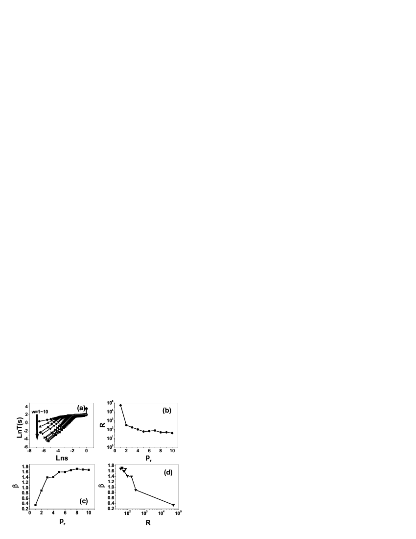
Figure 2: The relation of $\beta$ versus $R$ for the constructed BA scale-free networks. (a) Results for PDF of the NNLS. In the interested regions a brody distribution can capture the characteristics very well. (b) With the increase of $w$ the eigenratio $R$ decreases significantly. (c) With the increase of $w$ the parameter $\beta$ increases significantly. (d) The monotonous relation between the two parameters $\beta$ and $R$.

References

- (1) R. Albert, and A. -L. Barabasi, Rev. Mod. Phys. 74, 47(2002).
- (2) S. N. Dorogovtsev, and J. F. F. Mendes, Adv. Phys. 51, 1079(2002).
- (3) M. E. J. Newman, SIAM Review 45, 117(2003).
- (4) L. F. Lago-Fernndez, R. Huerta, F. Corbacho, and J. A. Siguenza, Phys. Rev. Lett. 84, 2758 (2000).
- (5) P. M. Gade, and C. -K. Hu, Phys. Rev. E 62, 6409 (2000).
- (6) X. F.Wang, and G. Chen, Int. J. Bifurcation Chaos Appl. Sci. Eng. 12, 187(2002).
- (7) M. Barahona, and L. M. Pecora, Phys. Rev. Lett. 89, 054101(2002).
- (8) P. G. Lind, J. A. C. Gallas, and H. J. Herrmann, Phys. Rev. E 70, 056207 (2004).
- (9) F. Liljeros, C. R. Edling, L. A. N. Amaral, H. E. Stanley, and Y. Aberg, Nature 411, 907 (2001).
- (10) H. Yang, F. Zhao, Z. Li, W. Zhang, and Y. Zhou, Int. J. Mod. Phys. B 18, 2734(2004).
- (11) B. -Y. Yaneer, and I. R. Epstein, Proc. Natl. Acad. Sci. 101, 4341(2004).
- (12) L. M. Pecora, and T. L. Carroll, Phys. Rev. Lett. 80, 2109(1998).
- (13) M. Barahona and L.M. Pecora, Phys. Rev. Lett. 89, 054101 (2002).; K. S. Fink, G. Johnson, T. Carroll, D. Mar, and L. Pecora, Phys. Rev. E 61, 5080 (2000).
- (14) T. Guhr, A. Mueller- Groeling, and H. A. Weidenmueller, Phys. Rep. 299, 189(1998).
- (15) V. Plerou, P. Gopikrishnan, B. Rosenow, L. A. N. Amaral, and T. Guhr, Phys. Rev. E 65, 066126(2002).
- (16) P. Seba, Phys. Rev. Lett. 91, 198104-1(2003).
- (17) H. Yang, F. Zhao, W. Zhang, and Z. Li, Physica A 347, 704(2005).
- (18) H. Yang, F. Zhao, Y. Zhuo, X. Wu, and Z. Li, Physica A 312, 23 (2002).
- (19) H. Yang, F. Zhao, Y. Zhuo, X. Wu, and Z. Li, Phys. Lett. A 292, 349 (2002).
- (20) S. N. Dorogovtsev, A. V. Goltsev, J. F. F. Mendes, and A. N. Samukhin, Phys. Rev. E 68, 046109(2003).
- (21) K. A. Eriksen, I. Simonsen, S. Maslov, and K. Sneppen, Phys. Rev. Lett. 90, 148701(2003).
- (22) K. -I. Goh, B. Kahng, and D. Kim, Phys. Rev. E 64, 051903 (2001).
- (23) I. J. Farkas, I. Derenyi, A.-L. Barabasi, and T. Vicsek, Phys. Rev. E 64, 026704(2001).
- (24) R. Monasson, Eur. Phys. J. B 12, 555 (1999).
- (25) H. Yang, F. Zhao, L. Qi, and B. Hu, Phys. Rev. E 69, 066104(2004).
- (26) F. Zhao, H. Yang, and B. Wang, Phys. Rev. E 72,046119(2005).
- (27) H. Yang, F. Zhao, and B. Wang, Physica A 364,544(2006).
- (28) M.A.M. de Aguiar and Yaneer Bar-Yam,Phys. Rev. E 71, 016106(2005).
- (29) P. W. Anderson, Phys. Rev. 109,1492(1958).
- (30) S. John, H. Sompolinsky, and M. J. Stephen, Phys. Rev. B 27, 5592(1983).
- (31) S. John, H. Sompolinsky, and M. J. Stephen, Phys. Rev. B 28,6358(1983).
- (32) S. John, H. Sompolinsky, and M. J. Stephen, Phys. Rev. Lett. 53,2169(1984).
- (33) T. A. Brody, J. Flores, J.B. French, P.A. Mello, A. Pandey, and S.S.M. Wong, Rev. Mod. Phys. 53, 385(1981).
- (34) T. Nishikawa, A. E. Motter,Y. C. Lai, and F. C. Hoppensteadt,Phys. Rev. Lett. 91,014101(2003).
- (35) H. Hong, M. Y. Choi, and B. J. Kim, Phys. Rev. E 65,026139(2002).
- (36) C. Zhou, A. E. Motter, and J. Kurths, Phys. Rev. Lett. 96,034101(2006).
- (37) H. Guclu, G. Korniss, M. A. Novotny, Z. Toroczkai, and Z. Racz, 73, 066115(2006).
- (38) D. J. Watts, S. H. Strogatz, Nature (London) 393, 440(1998).
- (39) A. -L. Barabasi, and A. Albert, Science 286, 509(1999).