Current fluctuations in a spin filter with paramagnetic impurities

Abstract

We analyze the frequency dependence of shot noise in a spin filter consisting of a normal grain and ferromagnetic electrodes separated by tunnel barriers. The source of frequency-dependent noise is random spin-flip electron scattering that results from spin-orbit interaction and magnetic impurities. Though the latter mechanism does not contribute to the average current, it contributes to the noise and leads to its dispersion at frequencies of the order of the Korringa relaxation rate. Under nonequilibrium conditions, this rate is proportional to the applied bias $V$, but parametrically smaller than $eV/\hbar$.

Recently, fundamental and applied aspects of spin-dependent transport attracted significant attention of physicists.Zutic-04 One of the prototype devices realizing this type of transport is a spin filter based on the use of ferromagnetic (FM) electrodes. In such a device, one of the electrodes may be viewed as ”polarizer” that generates a spin-polarized current and the other, the ”analyzer”, collects it. Current through the spin filter can drastically vary depending on the mutual orientation of electrode magnetizations.

An important characteristic of a mesoscopic device is its nonequilibrium noise,Blanter-00 which is due to randomness of electron transport and provides an important information about its nature. Fluctuations of current in a quantum dot with FM electrodes were considered in the Coulomb blockade regimeBulka-99 ; Bulka-00 and without it.Gurvitz-05 Nonequilibrium noise in a diffusive conductor with different mutual orientations of magnetizations in the leads was also studied.Tserkovnyak-01 More recently, several authors focused on the noise in diffusive spin filters caused by spin-flip scattering, which plays a crucial role in transport between electrodes with different magnetizations. This work was pioneered by Mishchenko,Mishchenko-03 who analyzed the noise in two-terminal diffusive spin filters for parallel and antiparallel magnetizations of electrodes and found a significant increase of shot noise in the latter case as compared to the conventional diffusive contacts. Calculations of shot noise caused by spin-flip scattering were also performed by other authors.Lamacraft-04 Shot noise and cross-correlations of current for multiterminal spin filters with spin-flip scattering were calculatedBelzig-04 ; Zareyan-05 as well. A frequency dependence of the shot noise in a quantum dot with spin-flip scattering connected with FM electrodes by ballistic point contacts was calculatedMishchenko-04 by Mishchenko et al.

In the absence of a magnetic field, spin-flip scattering in metals is dominated by spin-orbit processes and collisions of electrons with magnetic impurities. Though both these processes affect the spin of an individual electron and manifest themselves in weak-localization corrections to conductivity, only spin-orbit scattering contributes to the relaxation of average spin current; scattering off magnetic impurities conserves the total spin of the electron – impurity system and therefore the impurities eventually become polarized by incident electrons. The goal of the present paper is to study the relative importance of these two scattering mechanisms for the shot noise in spin filters. The principal difference between them is that the spin–orbit scattering changes only the spin of the electron and not the state of the ordinary impurity from which it is scattered. In contrast to this, spin-flip scattering off magnetic impurities results in a change of both impurity and electron spins thus affecting the ability of an impurity to flip an electron spin in the future. This results in impurity-induced correlations between electrons and therefore the spectral density of the noise of current should reflect their dynamics. Typically, the electron spin-orbit scattering time is much shorter than the time of spin-exchange scattering on paramagnetic impurities.Pierre-03 Therefore, the impurity spin-relaxation time should manifest itself in the frequency dependence of the noise spectrum. We calculate the spectrum of the noise in a spin filter at frequencies much smaller than the charge-relaxation time and show that it exhibits features characteristic of the impurity-spin relaxation.

I Equations for the averages

The system we consider consists of a normal-metal grain connected with two ferromagnetic electrodes via tunnel junctions with conductions much smaller than that of the grain yet larger than $e^{2}/\hbar$ so that Coulomb blockade does not occur. The level spacing is negligible compared to charging energy $e^{2}/C$ in a typical metallic grain. We also neglect the electron–phonon and electron–electron scattering. The polarizations of electrodes lead to spin-dependent tunneling rates, as the latter are proportional to the density of states of electrons with a given spin projection.

The average distribution functions of spin-up and spin-down electrons, $f_{\sigma}$ $(\sigma=\pm 1)$ are described by equations

$$\frac{\partial f_{\sigma}}{\partial t} = \Gamma_{L\sigma}[f_{0}(\varepsilon-eV/2)-f_{\sigma}]$$ (1)

$$+ \Gamma_{R\sigma}[f_{0}(\varepsilon+eV/2)-f_{\sigma}]$$

$$- \frac{1}{\tau_{so}}(f_{\sigma}-f_{-\sigma})+S_{\sigma}^{i}-e\frac{\partial U}{\partial t}\frac{\partial f_{\sigma}}{\partial\varepsilon}.$$

Here $\Gamma$’s are the tunneling rates through the left and right barriers for spin-up and spin-down electrons, $f_{0}(\varepsilon)$ is the equilibrium distribution function of electrons, $\tau_{so}$ is the spin-orbit scattering time, and $S_{\sigma}^{i}(\varepsilon)$ is the electron–impurity collision integral. The spin-flip part of the collision integral, evaluated in the lowest (second) order of perturbation theory in $J$, has the form

$$S_{\sigma}^{i}(\varepsilon)=J^{2}N_{F}[n_{\sigma}f_{-\sigma}(1-f_{\sigma})-n_{-\sigma}f_{\sigma}(1-f_{-\sigma})].$$ (2)

where $J$ is the constant of exchange interaction between the itinerant electrons and impurity spin, $N_{F}$ is the density of electron levels in the grain, $n_{\sigma}$ are concentrations of spin-up and spin-down impurities, and $U$ is the electric potential of the grain. All scattering processes accounted for in Eq. (1) are elastic (in the second order in $J$, relaxation of electron energy in scattering off magnetic impurities does not occurKaminski-01 ).

The relaxation of impurity spins in metals is also mainly due to interaction with electrons. In equilibrium, this mechanism is known as Korringa relaxationKorringa-50 and the corresponding relaxation rate is proportional to the electron temperature. In the case of an arbitrary electron distribution, the dynamics of impurities is described by a kinetic equation

$$\frac{\partial n_{\sigma}}{\partial t}=-N_{F}\int d\varepsilon\,S_{\sigma}^{i}.$$ (3)

This equation is compatible with the conservation law $\sum\limits_{\sigma=\pm 1}n_{\sigma}=n\equiv const$. The stationary solutions of these equations are found from the conditions

$$\frac{\partial f_{\sigma}}{\partial t}=0,\qquad\frac{\partial U}{\partial t}=0,\qquad S_{\sigma}^{i}=0.$$

It suggests that under the stationary conditions, the magnetic impurities do not affect the average distribution function of electrons and current. However they still contribute to the noise, as will be shown below.

II The Langevin equations

The dynamics of fluctuations is conveniently described by a set of coupled Langevin equations for the relevant distribution functions. Such equations are derived by varying properly the kinetic equations, and adding Langevin sources to the result of variations.Kogan For the spin filter we consider, the proper distribution functions are those of spin-up and spin-down electrons and magnetic impurities. The Langevin equations for these functions read

$$\Biggl{(} \frac{\partial}{\partial t}+\Gamma_{L\sigma}+\Gamma_{R\sigma}+\frac{1}{\tau_{so}}-\frac{\partial S_{\sigma}^{i}}{\partial f_{\sigma}}\Biggr{)}\delta f_{\sigma}$$ (4)

$$= \left(\frac{1}{\tau_{so}}+\frac{\partial S_{\sigma}^{i}}{\partial f_{-\sigma}}\right)\delta f_{-\sigma}+\frac{\partial S_{\sigma}^{i}}{\partial n_{\sigma}}\delta n_{\sigma}+\frac{\partial S_{\sigma}^{i}}{\partial n_{-\sigma}}\delta n_{-\sigma}$$

$$- e\frac{\partial f_{\sigma}}{\partial\varepsilon}\frac{\partial\delta U}{\partial t}-\delta j_{L\sigma}-\delta j_{R\sigma}+\delta F_{\sigma}^{so}+\delta F_{\sigma}^{i},$$

where $S_{\sigma}^{i}$ is given by Eq. (2) and $\delta j_{\alpha\sigma}$, $\delta F_{\sigma}^{so}=\sigma F_{so}$, and $\delta F_{\sigma}^{i}=\sigma F_{i}$ are Langevin sources related to tunneling of electrons with spin $\sigma/2$ through the left ($\alpha=L$) and right ($\alpha=R$) barriers, spin-orbit scattering, and spin-impurity scattering, respectively. The dynamics of the impurities is described by Langevin equations

$$\Biggl{[} \frac{\partial}{\partial t}+N_{F}\int d\varepsilon\,\left(\frac{\partial S_{\sigma}^{i}}{\partial n_{\sigma}}-\frac{\partial S_{\sigma}^{i}}{\partial n_{-\sigma}}\right)\Biggr{]}\delta n_{\sigma}$$ (5)

$$= -N_{F}\int d\varepsilon\,\left(\frac{\partial S_{\sigma}^{i}}{\partial f_{\sigma}}\delta f_{\sigma}+\frac{\partial S_{\sigma}^{i}}{\partial f_{-\sigma}}\delta f_{-\sigma}\right)$$

$$- N_{F}\int d\varepsilon\,\delta F_{\sigma}^{i},$$

where the relation $\delta n_{\sigma}=-\delta n_{-\sigma}$ was taken into account.

Fluctuations of the currents flowing into the left and right electrodes can be expressed in terms of $\delta f$ and $\delta j$,

$$\delta I_{\alpha}=eN_{F}\sum_{\sigma=\pm 1}\int d\varepsilon\,(\Gamma_{\alpha\sigma}\delta f_{\sigma}+\delta j_{\alpha\sigma}),\qquad\alpha=L,R.$$ (6)

To complete the set of equations, we relate the fluctuation of the electric potential of the grain $\delta U$, to the fluctuations of the currents flowing into the grain. Such relation follows from the charge conservation law and the definition of the electrostatic capacity of the grain $C$:

$$\frac{\partial}{\partial t}\delta U=-\frac{1}{C}(\delta I_{L}+\delta I_{R}).$$ (7)

It is natural to treat the Langevin sources $\delta j_{\alpha\sigma}$, $\delta F_{so}$, and $\delta F_{imp}$ as independent because they correspond to different scattering processes. As the scattering is assumed to be weak, it may be considered Poissonian, and the correlation functions of the Langevin sources in these equations may be written as the sums of outgoing and incoming scattering fluxes,

$$\langle\delta F_{so}(\varepsilon_{1},t_{1})\delta F_{so}(\varepsilon_{2},t_{2})\rangle=\delta(t_{1}-t_{2})\delta(\varepsilon_{1}-\varepsilon_{2})$$

$$\times\frac{1}{N_{F}\tau_{so}}\sum\limits_{\sigma=\pm 1}f_{\sigma}(\varepsilon_{1})[1-f_{-\sigma}(\varepsilon_{1})],$$ (8)

$$\langle\delta F_{imp}(\varepsilon_{1},t_{1})\delta F_{imp}(\varepsilon_{2},t_{2})\rangle=\delta(t_{1}-t_{2})\delta(\varepsilon_{1}-\varepsilon_{2})$$

$$\times\frac{J^{2}}{N_{F}}\sum\limits_{\sigma=\pm 1}n_{\sigma}f_{-\sigma}(\varepsilon_{1})[1-f_{\sigma}(\varepsilon_{1})],$$ (9)

$$\langle\delta j_{\alpha\sigma}(\varepsilon_{1},t_{1})\delta j_{\alpha\sigma}(\varepsilon_{2},t_{2})\rangle=\delta(t_{1}-t_{2})\delta(\varepsilon_{1}-\varepsilon_{2})$$

$$\times\frac{\Gamma_{\alpha\sigma}}{N_{F}}\Bigl{\{}f_{\sigma}(\varepsilon_{1})[1-f_{0}(\varepsilon_{1}-eV/2)]$$

$$+f_{0}(\varepsilon_{1}-eV/2)[1-f_{\sigma}(\varepsilon_{1})]\Bigr{\}}.$$ (10)

Equations (4) - (10) allow us to find the correlation functions of any observable quantity, e.g. of the current.

III Parallel magnetization of electrodes

First consider the case of a parallel magnetization of electrodes. Suppose that both left and right electrodes have spin-up magnetization so that only spin-up electrons can cross the interfaces with the normal metal. This can be modeled by setting $\Gamma_{L,-1}=\Gamma_{R,-1}=0$. The stationary solution of Eqs. (1) and (3) is

$$f_{\sigma}(\varepsilon)=\frac{\Gamma_{L1}f_{0}(\varepsilon-eV/2)+\Gamma_{R1}f_{0}(\varepsilon+eV/2)}{\Gamma_{L1}+\Gamma_{R1}},$$

$$n_{\sigma}=n/2.$$ (11)

As we are interested in frequencies much smaller than the inverse charge-relaxation time, we may set $C=0$ in Eq. (7), which reduces it to $\delta I_{L}+\delta I_{R}=0$. Together with Eqs. (6), this gives

$$\delta I_{L}=eN_{F}\int d\varepsilon\,\frac{\Gamma_{R1}\delta j_{L1}+\Gamma_{L1}\delta j_{R1}}{\Gamma_{L1}+\Gamma_{R1}}.$$ (12)

Making use of Eqs. (10) and (11), one readily obtains that in the low-temperature limit,

$$\langle\delta I_{L}^{2}\rangle_{\omega}=e^{3}N_{F}\frac{\Gamma_{L1}\Gamma_{R1}(\Gamma_{L1}^{2}+\Gamma_{R1}^{2})}{(\Gamma_{L1}+\Gamma_{R1})^{3}}V,$$ (13)

while the average current is

$$I=e^{2}N_{F}\frac{\Gamma_{L1}\Gamma_{R1}}{\Gamma_{L1}+\Gamma_{R1}}V.$$ (14)

These results suggest that for the parallel magnetizations of electrodes, neither the average current nor the noise are affected by spin-flip processes and the whole system behaves like a normal double tunnel junction with the density of states reduced by half. This is in a marked contrast with the case of a normal grain whose material has nonzero resistance,Mishchenko-03 where the spin-down sub-band in the grain contributes substantially to the current.

IV Antiparallel magnetization of electrodes

In the case of antiparallel magnetization of the leads, electron transport is associated with the spin-flip processes in the normal grain (we assume that the magnetization in the leads is saturated, and $\Gamma_{L,-1}=\Gamma_{R1}=0$). Considering for simplicity the case of symmetric junctions, $\Gamma_{L1}=\Gamma_{R,-1}=\Gamma$, we find

$$f_{\sigma}=\frac{(1+\Gamma\tau_{so})f_{0}(\varepsilon-\sigma eV/2)+f_{0}(\varepsilon+\sigma eV/2)}{2+\Gamma\tau_{so}}.$$ (15)

The steady impurity concentrations $n_{\sigma}$ are determined by setting $\partial n_{\sigma}/\partial t=0$ in Eq. (3), and accounting for the conservation condition $n_{\sigma}+n_{-\sigma}=n$,

$$\frac{n_{\sigma}}{n}=\frac{\int d\varepsilon\,f_{\sigma}(1-f_{-\sigma})}{\int d\varepsilon\,\sum\limits_{\sigma=\pm 1}f_{\sigma}(1-f_{-\sigma})}.$$ (16)

Our goal now is to obtain closed Langevin equations for fluctuations $\delta n_{\sigma}$ and $\delta U$ by eliminating $\delta f_{\sigma}$ from them. Then we can substitute the solutions of these equations back into the equation for $\delta f_{\sigma}$ and calculate the fluctuation of current.

Fluctuations of the distribution functions $\delta f_{\sigma}$ of the spin-up and spin-down electrons can be found from the Langevin equations (4)

$$\delta f_{\sigma}(\varepsilon,\omega) = \frac{-1}{-i\omega+\gamma_{\scriptscriptstyle\Sigma}(\varepsilon)}\Biggl{\{}\frac{1}{-i\omega+\Gamma}\Biggl{[}(-i\omega+\Gamma+\eta_{-\sigma})$$ (17)

$$\times \left(-i\omega\frac{\partial f_{\sigma}}{\partial\varepsilon}e\delta U+\sum\limits_{\alpha}\delta j_{\alpha\sigma}\right)$$

$$+ \eta_{-\sigma}\Biggl{(}-i\omega\frac{\partial f_{-\sigma}}{\partial\varepsilon}e\delta U+\sum\limits_{\alpha}\delta j_{\alpha,-\sigma}\Biggr{)}\Biggr{]}$$

$$- \frac{\partial S_{\sigma}^{i}}{\partial n_{\sigma}}\delta n_{\sigma}-\frac{\partial S_{\sigma}^{i}}{\partial n_{-\sigma}}\delta n_{-\sigma}+\delta F_{\sigma}^{so}+\delta F_{\sigma}^{i}\Biggl{\}},$$

where

$$\eta_{\sigma}=\frac{1}{\tau_{so}}-\frac{\partial S_{\sigma}^{i}}{\partial f_{\sigma}},$$

and

$$\gamma_{\scriptscriptstyle\Sigma}(\varepsilon)=\Gamma+\eta_{\sigma}+\eta_{-\sigma}$$

is the effective relaxation rate due both to tunneling and all types of spin-flip scattering. It follows from Eq. (15) that $1-f_{-\sigma}(\varepsilon)=f_{\sigma}(-\varepsilon)$, and therefore

$$\left.\frac{\partial S_{\sigma}^{i}}{\partial f_{\sigma}}\right|_{\varepsilon}=\left.\frac{\partial S_{-\sigma}^{i}}{\partial f_{-\sigma}}\right|_{-\varepsilon}.$$ (18)

Hence, $\eta_{\sigma}(\varepsilon)=\eta_{-\sigma}(-\varepsilon)$ and $\gamma_{\scriptscriptstyle\Sigma}(\varepsilon)=\gamma_{\scriptscriptstyle\Sigma}(-\varepsilon)$.

By substituting $\delta f_{\sigma}$ from Eq. (17) into Eq. (5), one obtains for the fluctuations of impurity polarization

$$\delta n_{\sigma} = \frac{\sigma N_{F}}{-i\omega+\Omega(\omega)}\int d\varepsilon\,\Biggl{[}(X-1)\delta F_{imp}+X\delta F_{so}$$ (19)

$$+ \sum\limits_{\alpha}\sum\limits_{\sigma=\pm 1}\sigma Y_{\sigma}(\varepsilon,\omega)\delta j_{\alpha\sigma}\Biggr{]}.$$

Here

$$\Omega(\omega)=N_{F}\int d\varepsilon\,\frac{-i\omega+\Gamma+2/\tau_{so}}{-i\omega+\gamma_{\scriptscriptstyle\Sigma}(\varepsilon)}\frac{\partial S_{1}^{i}}{\partial n_{1}}$$ (20)

gives at $\omega\to 0$ the inverse relaxation time of the impurity spins; coefficients

$$X(\varepsilon,\omega)=-\frac{1}{-i\omega+\gamma_{\scriptscriptstyle\Sigma}(\varepsilon)}\sum\limits_{\sigma=\pm 1}\frac{\partial S_{\sigma}^{i}}{\partial f_{\sigma}},$$ (21)

and

$$Y_{\sigma}(\varepsilon,\omega)=\frac{[1+\tau_{so}(-i\omega+\Gamma)]\partial S_{\sigma}^{i}/\partial f_{\sigma}+\partial S_{\sigma}^{i}/\partial f_{-\sigma}}{\tau_{so}(-i\omega+\Gamma)[-i\omega+\gamma_{\scriptscriptstyle\Sigma}(\varepsilon)]}$$ (22)

relate the fluctuations $\delta n_{\sigma}$ to Langevin sources. Note that $Y_{\sigma}(\varepsilon,\omega)=Y_{-\sigma}(-\varepsilon,\omega)$.

Using Eqs. (6) and (7) we now calculate $\delta U$

$$i\omega C\delta U=eN_{F}\int d\varepsilon\,\sum\limits_{\sigma=\pm 1}\left(\Gamma\delta f_{\sigma}+\sum\limits_{\alpha}\delta j_{\alpha\sigma}\right).$$ (23)

Substituting the sum of solutions from Eq. (17)

$$\sum\limits_{\sigma=\pm 1}\delta f_{\sigma}=-\frac{1}{-i\omega+\Gamma}\sum\limits_{\sigma=\pm 1}\left(-i\omega\frac{\partial f_{\sigma}}{\partial\varepsilon}e\delta U+\sum\limits_{\alpha}\delta j_{\alpha\sigma}\right)$$

into Eq. (23) and integrating out the derivatives, one obtains a closed expression for $\delta U$ in the formNagaev-04

$$\left(-i\omega+\Gamma+2\frac{e^{2}N_{F}\Gamma}{C}\right)\delta U=-\frac{eN_{F}}{C}\int d\varepsilon\,\sum\limits_{\alpha}\sum\limits_{\sigma=\pm 1}\delta j_{\alpha\sigma}.$$ (24)

Because the grain is sufficiently large, the second term in the parentheses in the left-hand side of Eq. (24) may be neglected as compared to the third term. The large coefficient $e^{2}N_{F}/C$ in the last term in parentheses is proportional to the ratio of the charging energy to the level spacing. As we are interested in frequencies much smaller than the inverse charge-relaxation time, Eq. (24) reduces to

$$\delta U=-\frac{1}{e\Gamma}\int d\varepsilon\,\sum\limits_{\alpha}\sum\limits_{\sigma=\pm 1}\delta j_{\alpha\sigma}.$$ (25)

Now we are able to express the fluctuation of current $\delta I_{L}$ in terms of Langevin sources $\delta J_{\alpha\sigma}$, $\delta F_{imp}$, and $\delta F_{so}$. For that, we substitute now Eq. (17) for $\delta f_{\sigma}$ into Eq. (6) for $\delta I_{L}$. Making use of the identity (18), one may eliminate the integration over $\varepsilon$. Substitution of $\delta U$ from Eq. (25) and $\delta n_{1}$ from Eq. (19) into the resulting expression gives

$$\delta I_{L} = eN_{F}\int d\varepsilon\,\Biggl{\{}\sum\limits_{\sigma=\pm 1}\Biggl{[}\sigma\frac{-i(\omega/2)(-i\omega+\gamma_{\scriptscriptstyle\Sigma})+\Gamma\eta_{\sigma}}{(-i\omega+\Gamma)(-i\omega+\gamma_{\scriptscriptstyle\Sigma})}$$ (26)

$$- \frac{\Gamma\Omega Y_{\sigma}(\varepsilon,\omega)}{(-i\omega+\Gamma+2/\tau_{so})(-i\omega+\Omega)}\Biggr{]}\sum\limits_{\alpha}\delta j_{\alpha\sigma}$$

$$+ \Gamma\Biggl{[}\frac{1}{-i\omega+\gamma_{\scriptscriptstyle\Sigma}}+\frac{\Omega(1-X)}{(-i\omega+\Gamma+2/\tau_{so})(-i\omega+\Omega)}\Biggr{]}$$

$$\times \delta F_{imp}+\Gamma\Biggl{[}\frac{1}{-i\omega+\gamma_{\scriptscriptstyle\Sigma}}\qquad$$

$$- \frac{\Omega X}{(-i\omega+\Gamma+2/\tau_{so})(-i\omega+\Omega)}\Biggr{]}\delta F_{so}\Biggl{\}}.$$

As the Langevin sources $\delta j_{\alpha\sigma}$, $\delta F_{imp}$, and $\delta F_{so}$ are independent, multiplying Eq. (26) by its complex conjugate and taking into account the expressions for the correlators of these sources (8) - (10), one obtains the spectral density of the noise as the sum of three terms related with the three types of scattering

$$\langle\delta I_{L}^{2}\rangle_{\omega}=\sum\limits_{\sigma=\pm 1}P_{\sigma}(\omega)+P_{so}(\omega)+P_{i}(\omega),$$ (27)

where

$$P_{\sigma}(\omega) = e^{2}N_{F}\Gamma\int d\varepsilon\,\Biggl{|}\frac{-i(\omega/2)(-i\omega+\gamma_{\scriptscriptstyle\Sigma})+\Gamma\eta_{\sigma}}{(-i\omega+\Gamma)(-i\omega+\gamma_{\scriptscriptstyle\Sigma})}$$ (28)

$$- \frac{\sigma\Gamma\Omega(\omega)Y_{\sigma}(\varepsilon,\omega)}{(-i\omega+\Gamma+2/\tau_{so})[-i\omega+\Omega(\omega)]}\Biggr{|}^{2}$$

$$\times \Bigl{\{}f_{\sigma}(\varepsilon)[1-f_{0}(\varepsilon-\sigma eV/2)]$$

$$+ f_{0}(\varepsilon-\sigma eV/2)[1-f_{\sigma}(\varepsilon)]\Bigr{\}},\quad$$

$$P_{so}(\omega) = \frac{e^{2}N_{F}\Gamma^{2}}{\tau_{so}}\int d\varepsilon\,\Biggl{|}\frac{1}{-i\omega+\gamma_{\scriptscriptstyle\Sigma}}$$ (29)

$$- \frac{\Omega(\omega)X(\omega)}{(-i\omega+\Gamma+2/\tau_{so})(-i\omega+\Omega)}\Biggr{|}^{2}$$

$$\times \sum\limits_{\sigma=\pm 1}f_{\sigma}(1-f_{-\sigma}),$$

and

$$P_{i}(\omega) = e^{2}N_{F}J^{2}\Gamma^{2}\int d\varepsilon\,\Biggl{|}\frac{1}{-i\omega+\gamma_{\scriptscriptstyle\Sigma}}$$ (30)

$$+ \frac{\Omega(\omega)[1-X(\omega)]}{(-i\omega+\Gamma+2/\tau_{so})(-i\omega+\Omega)}\Biggr{|}^{2}$$

$$\times \sum\limits_{\sigma=\pm 1}n_{\sigma}f_{-\sigma}(1-f_{\sigma}).$$

The general expressions Eqs. (27) - (30) for the spectral density are too cumbersome to be analyzed, and therefore we restrict ourselves to several interesting limiting cases. We assume that in all cases $T=0$.

The average current through the system is

$$I=\frac{e^{2}N_{F}\Gamma}{2+\Gamma\tau_{so}}V.$$ (31)

Note that $I\to 0$ at $\Gamma\tau_{so}\to\infty$ as no electron can pass through the filter without flipping its spin.

The noise properties of a system are often described by a frequency-dependent Fano factor $F=\langle\delta I_{L}^{2}\rangle_{\omega}/I$. In the absence of magnetic impurities, the Fano factor is

$$F=\frac{1}{2}e\frac{\tau_{so}^{2}(\omega^{2}+2\Gamma^{2})(2+\Gamma\tau_{so})+8(1+\Gamma\tau_{so})}{(2+\Gamma\tau_{so})[\omega^{2}\tau_{so}^{2}+(2+\Gamma\tau_{so})^{2}]}.$$ (32)

It exhibits positive dispersion for small $\Gamma\tau_{so}$ and negative dispersion for large $\Gamma\tau_{so}$ (see Fig. 1). Its dependence on the dwell time of an electron $1/\Gamma$ in the grain with tunnel junctions is different from the case of a grain with ballistic contactsMishchenko-04 both at zero and nonzero frequencies.

The presence of paramagnetic impurities leads to an additional frequency dispersion of the noise. The characteristic frequency $\omega_{0}$ of that dispersion is of the order of inverse spin-flip time for these impurities. At $T=0$ and within the lowest order perturbation theory in $J$, it is proportionalomega0 to the applied bias $V$ and therefore can be made much smaller than $\tau_{so}^{-1}$. In what follows, we will assume that this is the case. As the noise now depends on $V$ nonlinearly, it is more convenient to consider its full value rather than the Fano factor. In the limit $\Gamma\tau_{so}\ll 1$,

$$\Delta\langle\delta I_{L}^{2}\rangle_{\omega} \equiv \langle\delta I_{L}^{2}\rangle_{\omega}-\langle\delta I_{L}^{2}\rangle_{\infty}$$ (33)

$$= \frac{1}{8}e^{2}n(\Gamma\tau_{so})^{2}\frac{\omega_{0}^{3}(V)}{\omega^{2}+\omega_{0}^{2}(V)},$$

where $\omega_{0}(V)=eVN_{F}^{2}J^{2}/2$ is an analogue of inverse Korringa relaxation time with $eV$ in place of $T$. The low-frequency dispersion originates from the fluctuations of the number of spin-up and spin-down impurities, which modulate the overall spin-flip rate of electrons in the grain and result in fluctuations of the transport current. It is absent in the case of purely spin-orbit scattering.Mishchenko-04

For arbitrary values of $\Gamma\tau_{so}$, one can make use of the difference in the frequency scales between the spin-orbit and impurity-spin relaxations and isolate the part of $\langle\delta I_{L}^{2}\rangle_{\omega}$ that exhibits low-frequency dispersion. It has a form similar to Eq. (33)

$$\Delta\langle\delta I_{L}^{2}\rangle_{\omega}=e^{2}nA(\Gamma\tau_{so})\frac{\Omega^{3}(0)}{\omega^{2}+\Omega^{2}(0)},$$ (34)

with a modified spin-flip frequency of impurities

$$\Omega(0)=2\omega_{0}(V)B(\Gamma\tau_{so}),\qquad B(x)=\frac{1+(1+x)^{2}}{(2+x)^{2}}$$ (35)

and the dimensionless amplitude $A$ given by

$$A(x)=2\frac{x^{2}(1+x)(2+5x+x^{2})}{(2+x)^{3}[1+(1+x)^{2}]^{2}}.$$ (36)

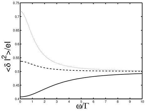
Figure 1: The frequency dependence of the Fano factor in the absence of magnetic impurities for $\Gamma\tau_{so}=1$ (solid line), $\Gamma\tau_{so}=4$ (dashed line), and $\Gamma\tau_{so}=10$ (dotted line).

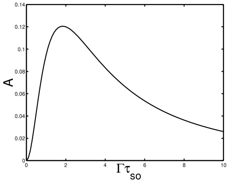
Figure 2: The amplitude of $\Delta\langle\delta I_{L}^{2}\rangle_{\omega}$ normalized to $e^{2}n\omega_{0}(V)$ vs. $\Gamma\tau_{so}$.

As $\Gamma\tau_{so}$ increases from 0 to infinity, the factor $B$ monotonically increases from 1/2 to 1. The dimensionless amplitude $A$ is plotted in Fig. 2 as a function of $\Gamma\tau_{so}$. It vanishes both at $\Gamma\tau_{so}\ll 1$ because in this case the two spin orientations become equivalent and the system behaves essentially as a one-sub-band conductor, and at $\Gamma\tau_{so}\gg 1$ because in this case the impurity spins become completely polarized and no spin-flip transitions take place.

V Summary

In summary, we have shown that paramagnetic impurities contribute to the shot noise in ferromagnet - normal metal - ferromagnet spin filters with opposite magnetizations of electrodes. Though their contribution to the noise is smaller than the contribution of spin-orbit scattering, it can be distinguished by a characteristic low-frequency dispersion that results from impurity-spin reorientations. As the rate of the impurity-spin relaxation depends on the energy distribution of electrons in the normal metal, this dispersion is affected by the applied voltage. Though the present calculations were performed for the ideal case of completely polarized electrodes, these effects also take place for more realistic systems with partial polarization.

- (1) I. Zǔtić, J. Fabian, and S. Das Sarma, Rev. Mod. Phys. 76, 323-410 (2004)
- (2) Ya. M. Blanter and M. Büttiker, Phys. Rep. 336, 1 (2000).
- (3) B. R. Bulka, J. Martinek, G. Michalek and J. Barnas, Phys. Rev. B 60, 12 246 (1999).
- (4) B. R. Bulka, Phys. Rev. B 62, 1186 (2000).
- (5) S. A. Gurvitz, D. Mozyrsky, and G. P. Berman, cond-mat/0506558.
- (6) Ya. Tserkovnyak and A. Brataas, Phys. Rev. B 64, 214402 (2001).
- (7) E.G. Mishchenko, Phys. Rev. B 68, 100409(R) (2003).
- (8) A. Lamacraft, Phys. Rev. B 69, 081301(R) (2004).
- (9) W. Belzig and M. Zareyan, Phys. Rev. B 69, 140407(R) (2004).
- (10) M. Zareyan and W. Belzig, Phys. Rev. B 71, 184403 (2005).
- (11) E. G. Mishchenko, A. Brataas, and Y. Tserkovnyak, Phys. Rev. B 69, 073305 (2004).
- (12) In recent low-temperature experiments on Au and Cu, was ns, and the spin-flip time related with magnetic impurities was several times larger even at their concentrations as high as 1 ppm, see F. Pierre, A. B. Gougam, A. Anthore, H. Pothier, D. Esteve, and N. O. Birge, Phys. Rev. B 68, 085413 (2003).
- (13) A. Kaminski and L. I. Glazman, Phys. Rev. Lett. 86, 2400 (2001).
- (14) J. Korringa, Physica 16, 601 (1950).
- (15) Sh. Kogan, Electronic Noise and Fluctuations in Solids, Cambridge University Press, 1996.
- (16) K. E. Nagaev, S. Pilgram, and M. Büttiker, Phys. Rev. Lett. 92, 176804 (2004).
- (17) It implies that bias is much larger than the Kondo temperature of the magnetic impurities in the given host metal.