Interpolation formula for the reflection coefficient distribution of absorbing chaotic cavities in the presence of time reversal symmetry

Abstract

We propose an interpolation formula for the distribution of the reflection coefficient in the presence of time reversal symmetry for chaotic cavities with absorption. This is done assuming a similar functional form as that when time reversal invariance is absent. The interpolation formula reduces to the analytical expressions for the strong and weak absorption limits. Our proposal is compared to the quite complicated exact result existing in the literature.

1 Introduction

In recent years there has been a great interest in the study of absorption effects on transport properties of classically chaotic cavities [1, 2, 3, 4, 5, 6, 7, 8, 9, 10, 11, 12, 13, 14, 15, 16, 17, 18] (for a review see Ref. [19]). This is due to the fact that for experiments in microwave cavities [20, 21], elastic resonators [22] and elastic media [23] absorption always is present. Although the external parameters are particularly easy to control, absorption, due to power loss in the volume of the device used in the experiments, is an ingredient that has to be taken into account in the verification of the random matrix theory (RMT) predictions.

In a microwave experiment of a ballistic chaotic cavity connected to a waveguide supporting one propagating mode, Doron et al [1] studied the effect of absorption on the $1\times 1$ sub-unitary scattering matrix $S$, parametrized as

$$S=\sqrt{R}\,e^{i\theta},$$ (1)

where $R$ is the reflection coefficient and $\theta$ is twice the phase shift. The experimental results were explained by Lewenkopf et al. [2] by simulating the absorption in terms of $N_{p}$ equivalent “parasitic channels”, not directly accessible to experiment, each one having an imperfect coupling to the cavity described by the transmission coefficient $T_{p}$.

A simple model to describe chaotic scattering including absorption was proposed by Kogan et al. [4]. It describes the system through a sub-unitary scattering matrix $S$, whose statistical distribution satisfies a maximum information-entropy criterion. Unfortunately the model turns out to be valid only in the strong-absorption limit and for $R\ll 1$. For the $1\times 1$ $S$-matrix of Eq. (1), it was shown that in this limit $\theta$ is uniformly distributed between 0 and $2\pi$, while $R$ satisfies Rayleigh’s distribution

$$P_{\beta}(R)=\alpha e^{-\alpha R};\qquad R\ll 1,\hbox{ and }\alpha\gg 1,$$ (2)

where $\beta$ denotes the universality class of $S$ introduced by Dyson [24]: $\beta=1$ when time reversal invariance (TRI) is present (also called the orthogonal case), $\beta=2$ when TRI is broken (unitary case) and $\beta=4$ corresponds to the symplectic case. Here, $\alpha=\gamma\beta/2$ and $\gamma=2\pi/\tau_{a}\Delta$, is the ratio of the mean dwell time inside the cavity ($2\pi/\Delta$), where $\Delta$ is the mean level spacing, and $\tau_{a}$ is the absorption time. This ratio is a measure of the absorption strength. Eq. (2) is valid for $\gamma\gg 1$ and for $R\ll 1$ as we shall see below.

The weak absorption limit ($\gamma\ll 1$) of $P_{\beta}(R)$ was calculated by Beenakker and Brouwer [5], by relating $R$ to the time-delay in a chaotic cavity which is distributed according to the Laguerre ensemble. The distribution of the reflexion coefficient in this case is

$$P_{\beta}(R)=\frac{\alpha^{1+\beta/2}}{\Gamma(1+\beta/2)}\frac{e^{-\alpha/(1-R)}}{(1-R)^{2+\beta/2}};\qquad\alpha\ll 1.$$ (3)

In the whole range of $\gamma$, $P_{\beta}(R)$ was explicitly obtained for $\beta=2$ [5]:

$$P_{2}(R)=\frac{e^{-\gamma/(1-R)}}{(1-R)^{3}}\left[\gamma(e^{\gamma}-1)+(1+\gamma-e^{\gamma})(1-R)\right],$$ (4)

and for $\beta=4$ more recently [13]. Eq. (4) reduces to Eq. (3) for small absorption ($\gamma\ll 1$) while for strong absorption it becomes

$$P_{2}(R)=\frac{\gamma\,e^{-\gamma R/(1-R)}}{(1-R)^{3}};\qquad\gamma\gg 1.$$ (5)

Notice that $P_{2}(R)$ approaches zero for $R$ close to one. Then the Rayleigh distribution, Eq. (2), is only reproduced in the range of few standard deviations i.e., for $R\stackrel{{\scriptstyle<}}{{\sim}}\gamma^{-1}$. This can be seen in Fig. 1(a) where we compare the distribution $P_{2}(R)$ given by Eqs. (2) and (5) with the exact result given by Eq. (4) for $\gamma=20$. As can be seen the result obtained from the time-delay agrees with the exact result but the Rayleigh distribution is only valid for $R\ll 1$.

Since the majority of the experiments with absorption are performed with TRI ($\beta=1$) it is very important to have the result in this case. Due to the lack of an exact expression at that time, Savin and Sommers [8] proposed an approximate distribution $P_{\beta=1}(R)$ by replacing $\gamma$ by $\gamma\beta/2$ in Eq. (4). However, this is valid for the intermediate and strong absorption limits only. Another formula was proposed in Ref. [16] as an interpolation between the strong and weak absorption limits assuming a quite similar expression as the $\beta=2$ case (see also Ref. [13]). More recently [17], a formula for the integrated probability distribution of $x=(1+R)/(1-R)$, $W(x)=\int_{x}^{\infty}P_{0}^{(\beta=1)}(x)dx$, was obtained. The distribution $P_{\beta=1}(R)=\frac{2}{(1-R)^{2}}P_{0}^{(\beta=1)}(\frac{1+R}{1-R})$ then yields a quite complicated formula.

Due to the importance to have an “easy to use” formula for the time reversal case, our purpose is to propose a better interpolation formula for $P_{\beta}(R)$ when $\beta=1$. In the next section we do this following the same procedure as in Ref. [16]. We verify later on that our proposal reaches both limits of strong and weak absorption. In Sec. 6 we compare our interpolation formula with the exact result of Ref. [17]. A brief conclusion follows.

2 An interpolation formula for $\beta=1$

From Eqs. (2) and (3) we note that $\gamma$ enters in $P_{\beta}(R)$ always in the combination $\gamma\beta/2$. We take this into account and combine it with the general form of $P_{2}(R)$ and the interpolation proposed in Ref. [16]. For $\beta=1$ we then propose the following formula for the $R$-distribution

$$P_{1}(R)=C_{1}(\alpha)\frac{e^{-\alpha/(1-R)}}{(1-R)^{5/2}}\left[\alpha^{1/2}(e^{\alpha}-1)+(1+\alpha-e^{\alpha}){}_{2}F_{1}\left(\frac{1}{2},\frac{1}{2},1;R\right)\frac{1-R}{2}\right],$$ (6)

where $\alpha=\gamma/2$, ${}_{2}F_{1}$ is a hyper-geometric function [25], and $C_{1}(\alpha)$ is a normalization constant

$$C_{1}(\alpha)=\frac{\alpha}{(e^{\alpha}-1)\Gamma(3/2,\alpha)+\alpha^{1/2}(1+\alpha-e^{\alpha})f(\alpha)/2}$$ (7)

where

$$f(\alpha)=\int_{\alpha}^{\infty}\frac{e^{-x}}{x^{1/2}}\,\,{}_{2}F_{1}\left(\frac{1}{2},\frac{1}{2},1;1-\frac{\alpha}{x}\right)$$ (8)

and $\Gamma(a,x)$ is the incomplete $\Gamma$-function

$$\Gamma(a,x)=\int_{x}^{\infty}e^{-t}t^{a-1}dt.$$ (9)

In the next sections, we verify that in the limits of strong and weak absorption we reproduce Eqs. (2) and (3).

3 Strong absorption limit

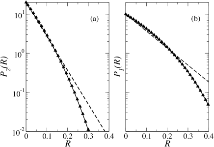
Figure 1: Distribution of the reflection coefficient for absorption strength $\gamma=20$, for (a) $\beta=2$ (unitary case) and (b) $\beta=1$ (orthogonal case). In (a) the continuous line is the exact result Eq. (4) while in (b) it corresponds to the interpolation formula, Eq. (6). The triangles in (a) are the results given by Eq. (5) for $\beta=2$ and in (b) they correspond to Eq. (11). The dashed line is the Rayleigh distribution Eq. (2), valid only for $R\stackrel{{\scriptstyle<}}{{\sim}}\gamma^{-1}$ and $\gamma\gg 1$.

In the strong absorption limit, $\alpha\rightarrow\infty$, $\Gamma(3/2,\alpha)\rightarrow\alpha^{1/2}e^{-\alpha}$, and $f(\alpha)\rightarrow\alpha^{-1/2}e^{-\alpha}$. Then,

$$\lim_{\alpha\rightarrow\infty}C_{1}(\alpha)=\frac{\alpha e^{\alpha}}{(e^{\alpha}-1)\alpha^{1/2}+(1+\alpha-e^{\alpha})/2}\simeq\alpha^{1/2}.$$ (10)

Therefore, the $R$-distribution in this limit reduces to

$$P_{1}(R)\simeq\frac{\alpha\,e^{-\alpha R/(1-R)}}{(1-R)^{5/2}}\qquad\alpha\gg 1,$$ (11)

which is the equivalent of Eq. (5) but now for $\beta=1$. As for the $\beta=2$ symmetry, it is consistent with the fact that $P_{1}(R)$ approaches zero as $R$ tends to one. It reproduces also Eq. (2) in the range of a few standard deviations ($R\stackrel{{\scriptstyle<}}{{\sim}}\gamma^{-1}\ll 1$), as can be seen in Fig. 1(b).

4 Weak absorption limit

For weak absorption $\alpha\rightarrow 0$, the incomplete $\Gamma$-function in $C_{1}(\alpha)$ reduces to a $\Gamma$-function $\Gamma(x)$ [see Eq. (9)]. Then, $P_{1}(R)$ can be written as

$$P_{1}(R) \simeq\frac{\alpha}{(\alpha+\alpha^{2}/2+\cdots)\Gamma(3/2)-(\alpha^{5/2}/2+\cdots)f(0)/2}$$ (12)

$$\times\frac{e^{-\alpha/(1-R)}}{(1-R)^{5/2}}\big{[}\alpha^{3/2}+\alpha^{5/2}/2+\cdots$$

$$-(\alpha^{2}/2+\alpha^{3}/6+\cdots){}_{2}F_{1}(1/2,1/2,1;R)(1-R)/2\big{]}.$$

By keeping the dominant term for small $\alpha$, Eq. (3) is reproduced.

5 Comparison with the exact result

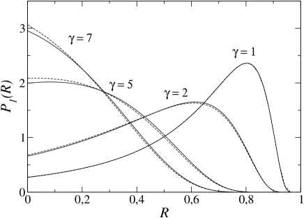
Figure 2: Distribution of the reflection coefficient in the presence of time-reversal symmetry for absorption strength $\gamma=1$, 2, 5, and 7. The continuous lines correspond to the distribution given by Eq. (6). For comparison we include the exact results of Ref. [17] (dashed lines).

In Fig. 2 we compare our interpolation formula, Eq. (6), with the exact result of Ref. [17]. For the same parameters used in that reference we observe an excellent agreement. In Fig. 3 we plot the difference between the exact and the interpolation formulas for the same values of $\gamma$ as in Fig. 2. The error of the interpolation formula is less than 4%.

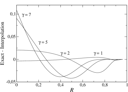
Figure 3: Difference between the exact result and the interpolation formula, Eq. (6), for the $R$-distribution for $\beta=1$ for the same values of $\gamma$ as in Fig. 2.

6 Conclusions

We have introduced a new interpolation formula for the reflection coefficient distribution $P_{\beta}(R)$ in the presence of time reversal symmetry for chaotic cavities with absorption. The interpolation formula reduces to the analytical expressions for the strong and weak absorption limits. Our proposal is to produce an “easy to use” formula that differs by a few percent from the exact, but quite complicated, result of Ref. [17]. We can summarize the results for both symmetries ($\beta=1$, 2) as follows

$$P_{\beta}(R)=C_{\beta}(\alpha)\frac{e^{-\alpha/(1-R)}}{(1-R)^{2+\beta/2}}\left[\alpha^{\beta/2}(e^{\alpha}-1)+(1+\alpha-e^{\alpha}){}_{2}F_{1}\left(\frac{\beta}{2},\frac{\beta}{2},1;R\right)\frac{\beta(1-R)^{\beta}}{2}\right],$$ (13)

where $C_{\beta}(\alpha)$ is a normalization constant that depends on $\alpha=\gamma\beta/2$. This interpolation formula is exact for $\beta=2$ and yields the correct limits of strong and weak absorption.

References

References

- [1] Doron E, Smilansky U and Frenkel A 1990 Phys. Rev. Lett. 65 3072
- [2] Lewenkopf C H, Müller A and Doron E 1992 Phys. Rev. A 45 2635
- [3] Brouwer P W and Beenakker C W J 1997 Phys. Rev. B 55 4695
- [4] Kogan E, Mello P A and Liqun He 2000 Phys. Rev. E 61 R17
- [5] Beenakker C W J and Brouwer P W 2001 Physica E 9 463
- [6] Schanze H, Alves E R P, Lewenkopf C H and Stöckmann H-J 2001 Phys. Rev. E 64 065201(R)
- [7] Schäfer R, Gorin T, Seligman T H, and Stöckmann H-J 2003 J. Phys. A: Math. Gen. 36 3289
- [8] Savin D V and Sommers H-J 2003 Phys. Rev. E 68 036211
- [9] Méndez-Sánchez R A, Kuhl U, Barth M, Lewenkopf C H and Stöckmann H-J 2003 Phys. Rev. Lett. 91 174102
- [10] Fyodorov Y V 2003 JETP Lett. 78 250
- [11] Fyodorov Y V and Ossipov A 2004 Phys. Rev. Lett. 92 084103
- [12] Savin D V and Sommers H-J 2004 Phys. Rev. E 69 035201(R)
- [13] Fyodorov Y V and Savin D V 2004 JETP Lett. 80 725
- [14] Hemmady S, Zheng X, Ott E, Antonsen T M and Anlage S M 2005 Phys. Rev. Lett. 94 014102
- [15] Schanze H, Stöckmann H-J, Martínez-Mares M and Lewenkopf C H, Phys. Rev. E 71 016223
- [16] Kuhl U, Martínez-Mares M, Méndez-Sánchez R A and Stöckmann H-J 2005 Phys. Rev. Lett. 94 144101
- [17] Savin D V, Sommers H-J and Fyodorov Y V 2005 Preprint cond-mat/0502359
- [18] Martínez-Mares M and Mello P A 2005 Phys. Rev. E 72 026224
- [19] Fyodorov Y V, Savin D V and Sommers H-J 2005 Preprint cond-mat/0507016
- [20] Alt H, Bäcker A, Dembowski C, Gräf H-D, Hofferbert R, Rehfeld H and Richter A 1998 Phys. Rev. E 58 1737
- [21] Barth M, Kuhl U and Stöckmann H-J 1999 Phys. Rev. Lett. 82 2026
- [22] Schaadt K and Kudrolli A 1999 Phys. Rev. E 60 R3479
- [23] Morales A, Gutiérrez L and Flores J 2001 Am. J. Phys. 69 517
- [24] Dyson F J 1962 J. Math. Phys. 3 1199
- [25] Abramowitz M and Stegun I A 1972 Handbook of Mathematical Functions (New York: Dover) chapter 15