Worm-like Polymer Loops and Fourier Knots

Abstract

Every smooth closed curve can be represented by a suitable Fourier sum. We show that the ensemble of curves generated by randomly chosen Fourier coefficients with amplitudes inversely proportional to spatial frequency (with a smooth exponential cutoff), can be accurately mapped on the physical ensemble of worm-like polymer loops. We find that measures of correlation on the scale of the entire loop yield a larger persistence length than that calculated from the tangent-tangent correlation function at small length scales. The conjecture that physical loops exhibit additional rigidity on scales comparable to the entire loop due to the contribution of twist rigidity, can be tested experimentally by determining the persistence length from the local curvature and comparing it with that obtained by measuring the radius of gyration of dsDNA plasmids. The topological properties of the ensemble randomly generated worm-like loops are shown to be similar to that of other polymer models.

Classical polymer theories, from Debye to Flory to De Gennes DeGennes and beyond, make extensive use of the analogy between conformation of a chain molecule and a Brownian random walk (BRW). In mathematically idealized form, such a random walk is thought of as a Wiener trajectory $\vec{r}(\tau)$ generated by the measure $P\left\{\vec{r}(\tau)\right\}\propto\exp\left[-\mathrm{const}{\displaystyle\int}\left(\partial\vec{r}/\partial\tau\right)^{2}d\tau\right]$, where $\tau$ is a parameter running along the trajectory. The BRW model brings powerful mathematical techniques, such as the diffusion equation, to bear on polymers but, however fruitful, this method has its limitations. For example, it is fundamentally unable to reproduce the fact of finite extensibility of polymer chains stretched by a strong forceMarcoSiggiaBustamante . Another field in which the Wiener trajectory model fails miserably is the study of polymers with knots. Indeed, simulations of discrete polymer models, or random polygons with $N$ steps, show N01 ; N02 ; N03 , that the probability of trivial knot configuration decays exponentially with $N$ as $P_{0}(N)\sim\exp\left(-N/N^{\ast}\right)$, where $N^{\ast}$ defines the crossover from an unknotted to a knotted regime. It was argued that Wiener trajectory polymer models can not be used to calculate this probability grosberg , since they correspond to the limit $N\rightarrow\infty$, $l\rightarrow 0$ ($l$ is a step length); $Nl^{2}=\mathrm{const}$, in which the probability of a trivial knot vanishes. Notice that the contour length of Wiener trajectory diverges, $Nl\rightarrow\infty$, so it is not surprising that these models do not exhibit finite extensibility. A better continuum model of polymers which can handle the constraints imposed both by finite extensibility and by the presence of knots, and can describe the elastic response of such objects, is that of a worm-like chain. However, while the statistical physics of linear worm-like polymers is well understood, little is known about the conformations and the topology of worm-like loops (WLL). Our goal in this article is to work out a method allowing computational generation of an ensemble of smoothly curved conformations of such polymers and to carry out the statistical analysis of their geometric and topological properties.

The conformations of worm-like polymers are generated by the measure $P\left\{\vec{r}(s)\right\}\propto\exp\left[-\mathrm{const}{\displaystyle\int}\left(\partial^{2}\vec{r}/\partial s^{2}\right)^{2}ds\right]$, subject to the constraint of non-extensibility, $\left|\partial\vec{r}/\partial s\right|=1$. That simply means that conformations are Boltzmann weighted by the bending energy proportional to the squared curvature. In more general elastic models RabinPanyukov , the three generalized curvatures describing the object could be treated as independent Gaussian variables. However, this is true only for linear (with open ends) filaments and attempts to generalize these methods to the case of closed loop failed because the loop closure conditions introduce a non-local coupling between the curvatures that makes the problem practically intractable (except for the case of small fluctuations of a planar ring in which this coupling can be explicitly taken into account ring ). One natural way to generate the conformations of a closed loop is to expand each component $r^{i}\left(\tau\right)$ in a Fourier series:

$$r^{i}\left(\tau\right)=\sum\limits_{n=1}\left[A_{n}^{i}\cos\left(\frac{2\pi n\tau}{T}\right)+B_{n}^{i}\sin\left(\frac{2\pi n\tau}{T}\right)\right]\ .$$ (1)

Here, $\tau$ is a parameter along the curve $\mathbf{r}(\tau)$ ($0\leq\tau\leq T$) and the summation goes up to some cutoff frequency $n_{\max}$ (if the series converges sufficiently rapidly, the cutoff can be replaced by infinity). Any conformation of a sufficiently smooth closed loop can be fully described by the set of Fourier coefficients $\left\{A_{n}^{i},B_{n}^{i}\right\}$, giving rise to the concept of Fourier knots introduced in Trautwein ; Kauffman . Notice that a Fourier knot is a much more general concept than the more traditional Lissajou knot, for which only one frequency is present for each coordinate direction.

Using the above prescription one can generate an ensemble of loops of different shapes by taking the Fourier coefficients from some random distribution. However, even though all the loops have the same period $T$, their contour lengths $L_{T}=\int_{0}^{T}d\tau^{\prime}\left|d\mathbf{r/}d\tau^{\prime}\right|$ are different for each realization of the Fourier coefficients. Even more importantly, since, in general, $\left|\partial\vec{r}/\partial\tau\right|\neq 1$, loops generated by (1) do not obey the inextensibility condition and can not be used to model worm-like polymers. In order to generate an ensemble of different conformations of an inextensible loop of some well-defined contour length, one has to transform to a representation in which trajectories are parametrized by the arclength $s$

$$s\left(\tau\right)=\int_{0}^{\tau}d\tau^{\prime}\left|d\mathbf{r/}d\tau^{\prime}\right|,\quad\text{with\quad}\left|\partial\vec{r}/\partial s\right|=1$$ (2)

and then bring all the generated conformations to the same contour length by a suitable affine transformation of all lengths and coordinates (this transformation does not affect the topology since the latter is independent of the parametrization). Thus, we can replace $L_{T}=s(T)$ by any standard length $L$, provided that we rescale all lengths using the affine transformation: $\mathbf{r}\rightarrow\mathbf{r}L/L_{T}$. Therefore, in three steps (generation of random coefficients and Fourier summation (1), reparametrization (2), and affine transformation $s\rightarrow sL/L_{T}$), of which the latter two couple all Fourier harmonics together in a complex way, we obtain a statistical ensemble of smoothly bent conformations of an inextensible loop of length $L$. Let us now check if this ensemble is representative of physical conformations of a worm-like loop which possesses some characteristic bending and (possibly) twist rigidities.

The first step is to recognize that on length scales much larger than some microscopic cutoff, the conformations of a worm-like polymer are well represented by those of a BRW. For the latter, the amplitudes of the Fourier components can be readily shown to be of the form $\left\{A_{n}^{i},B_{n}^{i}\right\}_{BRW}=\lambda/n$ for $n\leq n_{\max}$ and zero otherwise, where $\lambda$ is a random number (say, uniformly distributed between $-1$ and $1$; the choice of another symmetric interval is equivalent to rescaling the contour length, see below). As will be demonstrated in the following, short scale behavior characteristic of WLL can be obtained by replacing the abrupt cutoff $n_{\max}$ by Fourier coefficients that decrease smoothly with a characteristic decay frequency $n_{0}$,

$$\left\{A_{n}^{i},B_{n}^{i}\right\}_{WLL}=\lambda e^{-n/n_{0}}/n,$$ (3)

(notice that the WLL and the BRW expressions for the coefficients coincide for $n\ll n_{0}$).

The next step is to notice that the conformations of linear worm-like polymer are governed by the persistence length, which marks the cross-over between straight line conformations at small length scales and random walk type behavior at large length scales DeGennes . We expect that on small scales, the conformations of linear worm-like polymers and WLL are quite similar and that for the latter this cross-over is represented in Fourier space in terms of $n_{0}$. Of course, the analogy is meaningful only as long as $n_{0}\gg 1$, when there is a sufficiently broad range of length scales between the persistence length and the contour length of the knot. The characteristic property of the worm-like chain model is exponential decay (as $\exp(-s/l_{1})$) of the tangent-tangent correlation function, which defines the persistence length $l_{1}$; similarly, for WLL, on length scales sufficiently small compared to the entire loop, one expects that $\left\langle\left\langle t(s)\cdot t(0)\right\rangle\right\rangle\simeq\exp(-s/l_{1})$, where $\left\langle\left\langle{}\right\rangle\right\rangle$ denotes averaging both over the contour of a given loop and over the ensemble of loops. This expectation is confirmed in Figure 1a, where the logarithm of the correlation function is plotted against the dimensionless arclength $s/l_{1}$. The choice $l_{1}=0.43/n_{0}$ allows us to superimpose data for different values of $n_{0}$ in the range $30\leq n_{0}\leq 270$ (the small shift of the exponent is the result of the finite discretization of the contour length $s$).

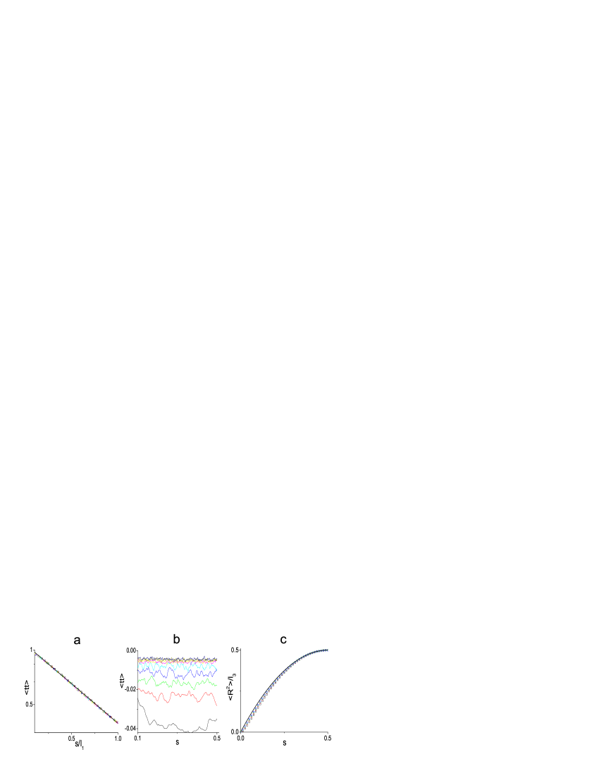
Figure 1: (Color online) (a) Universal semi-log plot of the short length scale behavior of the tangent-tangent correlation function vs the scaled distance, $s/l_{1}$; the best fit $exp(-(s/l_{1}-0.07))$ is given by the solid line. (b) Large scale behavior of the correlation function, for different values of $n_{0}$ (the height of the curves increases with $n_{0}$). (c) Scaled (by $l_{3}$) mean-squared distance between points on the loop. The BRW expression is plotted by the solid line. Different values of $n_{0}$ are represented by black ($n_{0}=30$), red ($n_{0}=50$), green ($n_{0}=70$), blue ($n_{0}=100$), cyan ($n_{0}=150$), magenta ($n_{0}=200$), yellow ($n_{0}=220$), dark yellow ($n_{0}=250$) and navy ($n_{0}=270$).

At first sight, analogy with worm-like chain models of linear polymers suggests that on length scales much larger than $l_{1}$ the conformations of the loops are those of BRW with step size (Kuhn length) given by twice the persistence length, $2l_{1}$. However, this analogy is open to question because the large scale behavior of a loop is strongly affected by the loop closure constraint and it is not clear, a’priori, whether the same persistence length controls both the small and the large scale behavior. We therefore decided to apply our method to generate a representative ensemble of configurations of WLL and use it to compute the tangent-tangent correlation function and the mean squared distance between two well-separated points $s$ and $s^{\prime}$ ($\left|s-s^{\prime}\right|\gg l_{1}$) along the contour.

A simple estimate shows that on length scales much larger than the persistence length, the tangent-tangent correlation function of a WLL approaches a constant negative value $\left\langle\left\langle t(s)\cdot t(0)\right\rangle\right\rangle\simeq-2l_{2}/L$ where $l_{2}$ is, in general,different from $l_{1}$ (the negative value of the correlation follows from the fact that the tangent has to turn back on itself in order to come back to its initial direction upon traversing the contour of the loop). In Fig. 1b this correlation function is plotted in the interval $0.1<s<0.5$ (here and in the following we take $L=1$) for different values of $n_{0}$. Upon averaging the correlation functions over the oscillations, all the results for different values of $n_{0}$ can be collapsed to a single horizontal line by dividing them by $l_{2}=0.575/n_{0}$. We therefore establish that unlike the case of linear worm-like chains in which only a single persistence length exists, WLL have at least two distinct persistence lengths, with $l_{1}/l_{2}\simeq 3/4$.

We now proceed to compute the mean squared distance between two points on the loop separated by a contour distance $s$, $\left\langle\langle R^{2}\left(s\right)\rangle\right\rangle=(1/L)\left\langle\int_{0}^{L}\left|\mathbf{r}\left(s^{\prime}+s\right)-\mathbf{r}\left(s^{\prime}\right)\right|^{2}ds^{\prime}\right\rangle$. Since we expect WLL to behave like BRW on scales much larger than some persistence length $l_{3}$, the probability distribution of $R^{2}(s)$ can be easily written down assuming that both $s\gg l_{3}$ and $L-s\gg l_{3}$. Apart from a normalization factor, this probability is equal to the product of two Gaussian functions: $\exp\left[-R^{2}/(2s\ell_{3})\right]\exp\left[-R^{2}/(2(L-s)\ell_{3})\right]$. Averaging with this distribution yields the well known relation (see, e.g., RedBook ), $\left\langle R^{2}\left(s\right)\right\rangle_{\mathrm{BRW}}=2l_{3}s\left(1-s/L\right).$ This result indicates that the plot of $\left.\langle\langle R^{2}(s)\rangle\rangle\right/l_{3}L$ against $\sigma=s/L$ is universal, i.e., it is the unit height parabola $4\sigma\left(1-\sigma\right)$, independent of either persistence length $l_{3}$ or total contour length $L$. Figure 1c shows that the data averaged over $1000$ different configurations collapse quite accurately on the expected parabolic master curve. Furthermore, by looking at our computational data for $\left\langle\left\langle R^{2}\left(s=L/2\right)\right\rangle\right\rangle$ averaged over all pairs of diametrically opposite points on the loop ($s=L/2=0.5$) we were able to relate the persistence length to the cutoff $n_{0}$. Within the accuracy of our simulation $l_{3}$ coincides with $l_{2}$ (see Fig. 2).

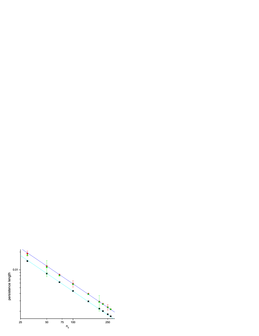
Figure 2: (Color online). Log-log plot of persistence lengths $l_{1},l_{2},l_{3}$ (black squares, green triangles and red circles respectively) vs $n_{0}$. The expressions $0.435/n_{0}$ and $0.57/n_{0}$ are shown as solid lines. The standard deviations are represented by error bars.

The conclusion that local and global statistical properties of worm-like loops are characterized by two different persistence lengths, $l_{1}$ and $l_{2}(=l_{3}),$ respectively, is a new result of this work. Although analytical theory of worm-like loops does not exist at present, we can offer some tentative considerations about the origin of the two persistence lengths, based on the study of small fluctuations of elastic rings ring . For rings of zero linking number that possess both bending and twist persistence lengths, it was shown that while on small scales writhe fluctuations depend only on the bending persistence length (on such scales the ring is essentially straight and bending and twist decouple), both bending and twist persistence lengths contribute to the writhe on larger scales, for which the global geometry of the closed ring becomes important. Extrapolating this result to the case of a strongly fluctuating loop considered in this work, suggests that while $l_{1}$ represents the pure bending contribution to the persistence length, $l_{2}$ contains both the bending and the twist contributions and is therefore larger than $l_{1}$ Mezard .

We now turn to the topological properties of WLL and examine the dependence of the trivial knot probability $P_{0}$ on the cutoff frequency $n_{0}$. Since $n_{0}$ determines the Kuhn length defined as either $2l_{1}$ or the $2l_{2}$, we can bring our knotting probability data to a form comparable to that for discrete polymer models, where trivial knot probability depends on the number of segments $N$. In our case, we generate Fourier knots as completely smooth curves, but we can define the number of effective segments as the ratio of the contour length to the Kuhn length. For long random–walk-like polymers, this definition coincides with the standard one accepted in polymer physics for the Kuhn segments RedBook but there remains an ambiguity associated with the choice of $N_{1}=L/2l_{1}$ or $N_{2}=L/2l_{2}$. In order to resolve this ambiguity we will measure the probability to obtain a trivial knot as a function of the cutoff frequency $n_{0}.$

To address the topology of the loops computationally, we employ the knot analysis routine due to R. Lua lua which identifies knots by computing the Alexander polynomial invariant $\Delta(t)$ at one value of argument, $t=-1$, and Vassiliev invariants of degrees two, $v_{2}$, and three, $v_{3}$. This set of invariants is widely considered as powerful enough for reliable identification of the trivial knot for all lengths achievable in practical computations. The details of this topological routine are described in lua .

The data on the trivial knot probability are shown in Figure 3. As this figure indicates, the trivial knot probability fits well to the exponential

$$P_{0}\left(n_{0}\right)\sim\exp\left[-n_{0}/242\right]\ .$$ (4)

Notice that since this relation involves only the cutoff on the Fourier series, formula (4) can be re-interpreted in purely mathematical form, not involving any references to polymers, or, for that matter, to any physics. While there is no fundamental understanding of the origin of this large cutoff ($n_{0}^{\ast}=242$) at present, our formulation hints at the existence of a hitherto unexplored connection between Fourier analysis and topology of space curves and will hopefully stimulate new work on this fundamental problem.

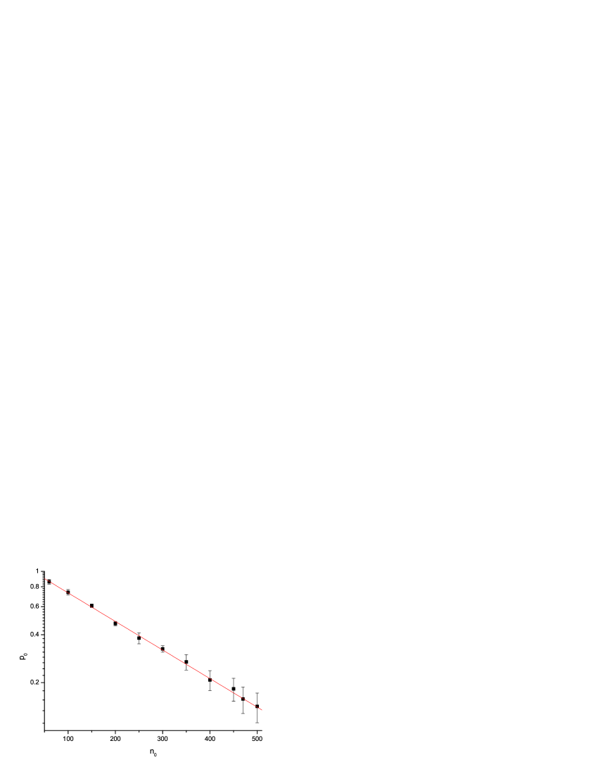
Figure 3: (Color online). Semi-log plot of the trivial knot probability as a function of $n_{0}$.

In summary, we have shown that the choice of random Fourier coefficients with amplitudes that decay with frequency as $n^{-1}\exp(-n/n_{0})$, generates a statistical ensemble of Fourier knots whose local properties coincide with those of worm-like polymers with persistence length that scales as $1/n_{0}$. We found that even though WLL behave on large scales as BRW as expected, the effective step size of this BRW is larger than that calculated from the local persistence length of the loop. This new prediction can be directly tested by experiments on double stranded DNA loops that can monitor both local (persistence length) and global (e.g., radius of gyration) properties of the polymers (see, e.g., AFM1 ; AFM2 ; SFM ). We also demonstrated that similar to discrete models of polymers or random polygons, our Fourier knots exhibit exponential decay of the unknotting probability with the number of effectively straight segments, or, equivalently, with the maximal spatial frequency included in Fourier expansion. The characteristic cross-over determined by this exponential decay represents a large number, which, although in the same ballpark as for other known models, remains an unexplained puzzle.

- (1) P.-G. De Gennes, Scaling Concepts in Polymer Physics (Cornell University Press, Ithaca, NY, 1979.
- (2) C. Bustamante, J. F. Marko, E. D. Siggia, and S. Smith, Science 265, 1599 (1994).
- (3) K. Koniaris and M. Muthukumar, Phys. Rev. Lett. 66, 2211-2214 (1991).
- (4) T. Deguchi, and K. Tsurusaki, Phys. Rev. E. 55, 6245-6248 (1997).
- (5) N.T. Moore, R. Lua, A.Y. Grosberg, Proc. Nat. Ac. Sci. 101, 13431 (2004).
- (6) A. Yu. Grosberg, Phys. Rev. Lett. 85, 3858-3861 (2000).
- (7) S. Panyukov and Y. Rabin, Phys. Rev. Lett. 85, 2404 (2000); Phys. Rev. E 62, 7135 (2000).
- (8) S. Panyukov and Y. Rabin, Phys. Rev. E 64, 011909 (2001).
- (9) A.Trautwein, Harmonic Knots Ph. D. Thesis, University of Iowa, 1995; Web Page: http://www2.carthage.edu/~trautwn/
- (10) L.H. Kauffman, Chapter 19 in: Ideal knots, A.Stasiak, V.Katrich, L.H.Kaufman - Editors (World Scientific, Singapore, 1998).
- (11) A. Yu. Grosberg and A. R. Khokhlov, Statistical Physics of Macromolecules (AIP Press, NY, 1994).
- (12) R. Lua, A. Borovinskiy and A. Yu. Grosberg, Polymer 45, 717 (2004).
- (13) This effect is expected only for worm-like loops; for linear worm-like chains it can be shown that twist degrees of freedom can be integrated over and that the spatial conformations of the polymer depend on the bending rigidity only: C. Bouchiat and M. Mezard, Eur. Phys. J. E 2, 377 (2000).
- (14) Y.L. Lyubchenko and L.S. Shlyakhtenko, Proc. Natl. Acad. Sci. USA 94, 496 (1997).
- (15) A. Scipioni et al., Chemistry & Biology 9, 1315 (2002)
- (16) M. Bussiek, N. Mücke and J. Langowski, Nucleic Acids Research 31, e137 (2003).