Abstract

Ground state of the quantum Jahn-Teller model with broken rotational symmetry was investigated by the variational approach in two cases: a lattice and a local ones. Both cases differ by the way of accounting for the nonlinearity hidden in the reflection-symmetric Hamiltonian. In spite of that the ground state energy in both cases shows the same features: There appear two regions of model parameters governing the ground state: the region of dominating selftrapping modified by the quantum effects and the region of dominating phonon-assisted tunneling (antiselftrapping). In the local case (i) the effect of quantum fluctuations and anharmonicity due to the two-mode correlations is up to two orders larger than contributions due to the reflection effects of two-center wave function; (ii) the variational results for the ground state energy were compared with exact numerical results. The coincidence is the better the more far away from the transition region at the E$\otimes$e symmetry where the variational approach fails.

List of Content

1. Introduction

2. Extended (lattice) generalized Jahn-Teller model

3. Ground state of the lattice model

4. Ground state of the local model

5. Discussion of the numerical results

6. Quantum fluctuations in the local model

7. Conclusion

1 Introduction

Jahn-Teller model as a protopype model for phonon removal of degeneracy of electron levels in complex molecules [1] was investigated mainly in its rotational symmetric E$\otimes$e local version with electron coupling to two degenerate intramolecular phonon modes, one antisymmetric and one symmetric against reflection.Importance of focusing on the lattice version of the model increased due to JT-based structural phase transitions in some recently discovered high-$T_{c}$ superconductors and manganese-based perovskites [2], [3].

For the reflection symmetric two-level electron-phonon models with linear coupling to one phonon mode (exciton, dimer) Shore et al. [4] introduced variational wave function in a form of linear combination of the harmonic oscillator wave functions related with two levels. Two asymmetric minima of effective polaron potential turn coupled by a variational parameter respecting its anharmonism by assuming two-center variational phonon wave function. This approach was shown to yield the lowest ground state energy for the two-level models [4], [5].

The peculiarities due to reflection phenomena are also expected in the case of linear coupling with two phonon modes. In contrast to the model with coupling to one phonon mode, the oscillations mediated by the antisymmetric mode are nonlinearly coupled to the symmetric phonon mode. Therefore, in order to improve the harmonic oscillator variational ansatz for this model, it was necessary to introduce additional variational parameters (VP) considering correlation of both phonon modes. This was performed by Lo [6] for the E$\otimes$e JT model and by Lo et al. [7]) for the dimer model. The correlation was found most effective in the region of parameters where the competing localization (polaron) energy and the delocalization transfer energy (tunneling) were comparable.

In crystals exhibiting high space anisotropy the rotational symmetry of Jahn-Teller molecules can be broken. Therefore it is reasonable to investigate JT model generalized by breaking the rotational symmetry (while saving the reflection symmetry): we assume different coupling strengths for the onsite (intralevel) and interlevel electron-phonon couplings. Such a model can also be considered as a generalization of the exciton-phonon or the dimer-phonon model by assuming the electron tunneling phonon assisted. JT model with the broken rotational symmetry will involve the coupling of two minima as well as the coupling of the symmetric and antisymmetric phonon modes. In the lattice model, however, in contrast to the local case, the mode correlation appears to be of a marginal importance (Section III). As a consequence, our ansatz for the variational wave function of the local model will involve (i) the reflection VP introduced by the construction of the two-center phonon wave function, and (ii) correlation VP respecting coupling of the symmetric and antisymmetric phonon modes. The question arises of the importance of these VPs and respective effects regarding their relevance in different regions of the model parameters. Formulation of the variational ansatz of the local case is presented in the Section IV. Calculation of the ground state energy of the lattice model and related discussions are the contents of the Sect.III. and V. Reliability of different variational alternatives was checked by comparison with results of exact numerical simulations for the local model.

2 Extended (lattice) generalized Jahn-Teller model

We investigate 1D lattice of spinless double degenerated electron states linearly coupled to two intramolecular phonon modes described by Hamiltonian

$$H=\Omega\sum_{n,i=1,2}(b_{i,n}^{{\dagger}}b_{i,n}+1/2)+\sum\limits_{n}\left(\alpha(b_{1,n}^{{\dagger}}+b_{1,n})\sigma_{zn}\right.$$

$$\left.-\beta(b_{2,n}^{{\dagger}}+b_{2,n})\sigma_{xn}\right)-\frac{T}{2}\sum_{n,j=1,2}(R_{1,j}+R_{-1,j})I_{n}\,.$$ (1)

where $b_{i,n},i=1,2$ are phonon annihilation operators, and the Pauli matrices $\sigma_{ln}$ represent two-level electron system. They satisfy identities $\ [\sigma_{ln},\sigma_{jn}]=i\sigma_{kn},\ l=x,y,z$, representing $1/2$-pseudo-spins related to the electron densities in a usual way, i.e. $\sigma_{xn}=\frac{1}{2}(c^{{\dagger}}_{1,n}c_{2,n}+c^{{\dagger}}_{2,n}c_{1,n}),\$ $\sigma_{yn}=\frac{1}{2i}(c^{{\dagger}}_{1,n}c_{2,n}-c^{{\dagger}}_{2,n}c_{1,n}),$ $\sigma_{zn}=\frac{1}{2}(c^{{\dagger}}_{1,n}c_{1,n}-c^{{\dagger}}_{2,n}c_{2,n}),$ $\ I_{n}=\frac{1}{2}(c^{{\dagger}}_{1,n}c_{1,n}+c^{{\dagger}}_{2,n}c_{2,n})$ is a unit matrix, and $c_{j,n}$ are electron annihilation operators. The operator $R_{\pm 1,j}=e^{\pm ipa}$ of the displacement by a lattice constant $\pm a$ acts in both the electron and phonon space, $R_{\pm 1,j}f_{n}=f_{n\pm 1}R_{\pm 1,j}$.

In terms of the creation-annihilation electron and phonon operators the Hamiltonian can be cast as follows:

$$H=\sum_{n}[\Omega\sum_{i=1,2}(b_{in}^{{\dagger}}b_{in}+\frac{1}{2})+\frac{\alpha}{2}(c^{{\dagger}}_{1,n}c_{1,n}-c^{{\dagger}}_{2,n}c_{2,n})(b_{1n}^{{\dagger}}+b_{1n})$$

$$-\frac{\beta}{2}(c_{1n}^{{\dagger}}c_{2n}+c_{2n}^{{\dagger}}c_{1n})(b_{2n}^{{\dagger}}+b_{2n})-\frac{T}{2}\sum_{j=1,2}(c_{j,n}^{{\dagger}}c_{j,n+1}+H.c.)]\,.\qquad$$ (2)

For $\beta=-\alpha$, the interaction part of (1)

$$\alpha\left(\matrix{b_{1n}^{{\dagger}}+b_{1n},\ b_{2n}^{{\dagger}}+b_{2n}\cr b_{2n}^{{\dagger}}+b_{2n},\ -(b_{1n}^{{\dagger}}+b_{1n})}\right)$$ (3)

yields the rotationally symmetric $E\otimes e$ form [1] with a pair (an antisymmetric and a symmetric under reflection) of double degenerated vibrations. This is, e.g., the case of $Cu^{++}$ ions with $d^{9}$ configurations in high-$T_{c}$ cuprates [1],[2].

Taking $\alpha\neq\beta$ removes the degeneration of the vibronic states breaking the rotational symmetry of the electron-phonon interactions, the model still staying within the class of JT models [1], [2].

The dispersionless optical phonon mode $b_{1}$ splits the degenerated unperturbed electron level ($j=1,2$) while the mode $b_{2}$ mediates the electron transitions between the levels. This latter term represents phonon-assisted tunneling, a mechanism of the nonclassical (nonadiabatic) nature as well as is the pure tunneling in related exciton and dimer models.

Evidently, Hamiltonian (1) ($\alpha\neq\beta$) is reflection-symmetric, $G^{(el)}G_{1}^{(ph)}H=H$,

$$|2\rangle = G^{(el)}|1\rangle,\ (G^{(el)})^{2}=1,$$

$$G^{(ph)}_{1n}(b_{1n}^{{\dagger}}\pm b_{1n}) = -(b_{1n}^{{\dagger}}\pm b_{1n})G^{(ph)}_{1n},\ (G^{(ph)}_{1n})^{2}=1,$$ (4)

where $G^{(ph)}_{1n}=\exp(i\pi b^{{\dagger}}_{1n}b_{1n})$ is the phonon reflection operator. While the phonon $1$ is antisymmetric under the reflection, phonon $2$ remains symmetric.

In addition, the transfer part of (2) exhibits $SU(2)$ symmetry of the left- and right-moving electrons (holes).

Let us note that the quantum phonon assistance of the electron tunneling ($\beta$-term in (2) and (1)) constitutes the difference of the model from the related dimer and exciton quantum models where instead of $\beta\sum\limits_{n}(b_{2n}^{{\dagger}}+b_{2n})\sigma_{xn}$ of (1) there stands $\Delta\sigma_{xn}$, where $\Delta$ is the distance between the levels [4],[5].

The local part of (1) can be diagonalized in electron subspace by the Fulton-Gouterman unitary operator [8] $U_{n}\equiv U_{2,n}U_{1,n}$, where

$$U_{i,n}=\frac{1}{\sqrt{2}}\left(\matrix{1\ ,\ G_{i,n}\cr 1\ ,\ -G_{i,n}}\right),\quad G_{i,n}=\exp(i\pi b_{in}^{{\dagger}}b_{in})\equiv G^{(ph)}_{i,n},$$ (5)

as follows

$$\tilde{H}_{L}=\sum\limits_{n}U_{n}H_{0n}U_{n}^{-1}=\Omega\sum\limits_{n,i=1,2}\left(b_{in}^{{\dagger}}b_{in}+\frac{1}{2}\right)$$

$$+\frac{1}{2}\sum\limits_{n}[\alpha(b_{1n}^{{\dagger}}+b_{1,n})-\beta(b_{2n}^{{\dagger}}+b_{2n})G_{1,n})]I_{n}.$$ (6)

On the other hand, in the transfer term

$$\tilde{H}_{T}=-\frac{T}{2}\sum_{n}\left(V_{n,1}R_{1}+V_{n,-1}R_{-1}\right)$$ (7)

there appears a nondiagonality

$$V_{n,\pm 1}=\left[(1+G_{1n}G_{1n\pm 1})I_{n}+(1-G_{1n}G_{1,n\pm 1})G_{2n}\sigma_{zn}\right]$$

$$\times\left[(1+G_{2n}G_{2n\pm 1})I_{n}+(1-G_{2n}G_{2,n\pm 1})\sigma_{xn}\right].\qquad$$ (8)

Here, Pauli matrices transform as $U_{i}\sigma_{x}U_{i}^{-1}=G_{i}\sigma_{z}$, $U_{i}\sigma_{z}U_{i}^{-1}=\sigma_{x}$, and $U_{i}(b_{i}^{{\dagger}}+b_{i})U^{-1}_{i}=(b_{i}^{{\dagger}}+b_{i})2\sigma_{x}$.

The diagonal terms of (8) represent the polaron transfer within one level while the off-diagonal ones represent the interlevel polaron transfer through the lattice. Evidently, the contribution of the off-diagonal terms proportional to $1-G_{in}G_{i,n+1}$ is much smaller when compared with those proportional to $1+G_{in}G_{i,n+1}$.

Because of nonconservation of the number of coherent phonons, they are able even in the ground state to assist electron transitions between the levels. In the Hamiltonian (6), the operator $G_{1n}=(-1)^{b_{1n}^{{\dagger}}b_{1n}}$ (5), highly nonlinear in the phonon-$1$ appears mediated by phonons $2$. It introduces multiple electron oscillations between the split levels mediated by continuous virtual absorption and emission of the phonons $1$. The effect is analogous to Rabi oscillations in quantum optics due to photons [9]. Let us note that Rabi oscillations assist both the interlevel onsite and intersite electron transitions mediated by the electron transfer $T$.

Further we shall investigate by variational approach the two variants of the model (1) - the lattice and the local one (considering $T=0$).

Shore et al [4] and Wagner et al [5] proved for exciton or dimer models coupled to one phonon mode that the two-center wave function generalized to an asymmetric nonunitary ansatz with a variational parameter $\eta$ of a form

$$\Psi^{(p)}=\frac{1}{\sqrt{C}}(1+\eta pG)|1\rangle\phi^{(p)},$$ (9)

(where $C$ is a normalization constant), yields lower ground state [4], [5].

So, rather generally we define phonon wave functions $\phi^{(p)}$

$$\phi^{(\pm)}=D_{1}(\pm\zeta_{1})D_{2}(\zeta_{2})S_{2}(r_{2})S_{1}(r_{1})S_{12}(\pm\lambda)|0\rangle.$$ (10)

Here, the generators of variational displacements are defined

$$D_{i}(\eta)=\exp[\zeta_{i}(b_{i}^{{\dagger}}-b_{i})],$$ (11)

and those of squeezing

$$S_{i}(r_{i})=\exp[r_{i}(b_{i}^{{\dagger}2}-b_{i}^{2})],$$ (12)

for $i=1,2$. In Eq. (6) coupling of the phonon modes $1$ and $2$ occurs, therefore one includes into the ansatz (10) also the correlation generator

$$S_{12}(\lambda)=\exp[\lambda(b_{1}^{{\dagger}}b_{2}^{{\dagger}}-b_{1}b_{2})].$$ (13)

with a correlation VP $\lambda$.

The form (10) is written here seemingly for the local case, while the most general form of it should contain the dependencies of all variational parameters on $n$ (site number in the lattice): $\gamma_{1}\to\gamma_{1m}(n)$ etc, showing the displacement of the mode $1$ at the site $m$ due to the electron at the site $n$, $\gamma_{jm}(n)=\frac{1}{\sqrt{N}}\sum\limits_{q}\gamma_{jq}(n)\exp(-iqma)$. We take

$$\gamma_{jq}(n)=\frac{\gamma_{j}}{\sqrt{N}}\exp(iqna)\rightarrow\gamma_{jm}(n)=\gamma_{j}\delta_{m,n},$$ (14)

where $\gamma_{j}$ are independent of $n$. Eq. (14) indicates that the phonon displacement accompanies the electron at the site $n$. The same is valid for the squeezing, $r_{m}(n)=r\delta_{m,n}$ and mixing parameter $\lambda$. When we consider the ground state of the lattice model, we omit the electron and phonon dynamic terms by setting $k=0$, $q=0$, thus even in the lattice case we are left with the effective local molecule Hamiltonian, the only difference being the additional contribution of the transfer terms (those containing $T$). As it is shown later, in the lattice model we can set $\lambda=0$ without worsening considerably the variational results, while for the local case $T=0$ introducing this parameter considerably improves the results. In what follows the ground state energy as function of optimized variational parameters $\eta$, $\gamma_{1},\gamma_{2},r,\lambda$ will be determined.

3 Ground state of the lattice model

First we consider the lattice model setting $\lambda=0$.

By averaging $\tilde{H}=\tilde{H}_{L}+\tilde{H}_{T}$ ((6), (7)) over the phonon wave functions (9) with (10) one obtains for the site Hamiltonian (6) the local part in the form

$$\frac{\langle\tilde{H}_{L}\rangle}{N}\equiv H_{ph}+H_{int},$$ (15)

where

$$H_{ph}=\frac{\Omega}{2}(\cosh 4r+1)I+\Omega\frac{1+\eta^{2}-2\eta e^{-8r_{1}}\exp(-2|\tilde{\gamma}_{1}|^{2})}{1+\eta^{2}+2\eta\exp(-2|\tilde{\gamma}_{1}|^{2})}|\gamma_{1}|^{2}I+$$

$$+\Omega|\gamma_{2}|^{2}I,$$ (16)

$$H_{int}\equiv H_{\alpha}+H_{\beta}=\frac{\alpha(1-\eta^{2})}{1+\eta^{2}+2\eta\exp(-2|\tilde{\gamma}_{1}|^{2})}\gamma_{1}\sigma_{z}-$$

$$-\frac{\beta[(1+\eta^{2})\exp(-2|\tilde{\gamma}_{1q}|^{2})+2\eta]}{1+\eta^{2}+2\eta\exp(-2|\tilde{\gamma}_{1}|^{2})}\gamma_{2}I\,,$$ (17)

where $H_{\alpha}$ and $H_{\beta}$ are $\alpha$- and $\beta$-dependent parts of the interaction $H_{int}$ (17). From the transfer Hamiltonian $\tilde{H}_{T}$ (7) there remains

$$\frac{\langle\tilde{H}_{T}\rangle}{N}=-T\exp(-W)M\equiv 2(H_{T1}I+H_{T2}i\sigma_{y}+H_{T3}\sigma_{z}+H_{T4}\sigma_{x}).$$ (18)

where $M$:

$$M=\left[(1+E_{1}^{2})I+(1-E_{1}^{2})E_{2}\sigma_{zn}\right].\left[(1+E_{2}^{2})I+(1-E_{2}^{2})\sigma_{x}\right],$$ (19)

and $E_{i}$ are given by

$$E_{1}\equiv\exp\left(-2|\tilde{\gamma}_{1}|^{2}\right),\ E_{2}\equiv\exp\left(-2|\gamma_{2}|^{2}\right).$$ (20)

Expressions $E_{i}$ (20) in the ground state are independent of $q$ and $n$ because of the form of $\gamma_{iq}(n)=\gamma_{i}\exp(-iqna)$ (14). This substantially simplifies subsequent calculations leaving $E_{i}$ and $C_{1}$ as functions of $\gamma_{i}^{2}$ independent on $n$. The transfer terms $H_{Ti},\ i=1,2,3,4$ in (18) with (19) are expressed as

$$H_{T1}=-\frac{T}{4}(1+E_{1}^{2})(1+E_{2}^{2}),\quad H_{T2}=-\frac{T}{4}(1-E_{1}^{2})(1-E_{2}^{2})E_{2},$$

$$H_{T3}=-\frac{T}{4}(1-E_{1}^{2})(1+E_{2}^{2})E_{2},\quad H_{T4}=-\frac{T}{4}(1+E_{1}^{2})(1-E_{2}^{2}).$$ (21)

Here, $H_{T1},H_{T3}$ and $H_{T2},H_{T4}$ are diagonal and off-diagonal terms of (18), respectively.

The effective polaron potential in (15) (with (16)-(20)) as a highly nonlinear function of $\gamma_{1}$ and $\gamma_{2}$ is visualized in Fig. 1.

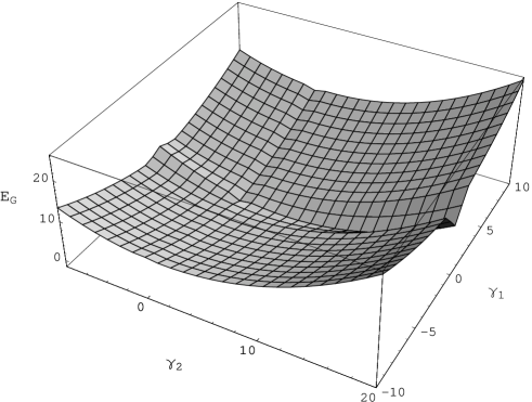
Figure 1: The effective potential for $\chi=\beta/\alpha=0.5,\mu=2$ and $T=1,\Omega=0.05$ as function of $\gamma_{1}$, $\gamma_{2}$.

The potential exhibits two sets of minima related to two competing ground states:
(i) Two nonequivalent broad minima related to both the levels (10) at $\pm\gamma_{1}\neq 0$ and $\gamma_{2}$ close to $0$;
(ii) One narrow minimum at $\gamma_{1}$ close to $0$, $\gamma_{2}>0$, where both levels approach close together. This minimum develops at growing $\beta$; evidently its behaviour depends also on $T$ value because of nonlinearity of the Debye-Waller factor $M$ ((19) and (20)).

The ground state energies related to these two sets of competing minima were calculated numerically. The result of the numerical minimalization of the diagonalized form of energy (15)

$$E=H_{ph}+H_{\beta}+H_{T_{1}}-\left[(H_{\alpha}+H_{T_{3}})^{2}+H^{2}_{T_{4}}-H^{2}_{T_{2}}\right]^{1/2}$$ (22)

can be written symbolically as

$$E_{G}(\mu,\chi,\Omega/T)=E(\{\gamma_{1q},\gamma_{2q},r,\eta\}_{min})/T.$$ (23)

Here, the index $min$ denotes the optimized values. The model parameters

$$\mu=\frac{\alpha^{2}}{2\Omega T},\quad\chi=\frac{\beta}{\alpha},\quad\frac{\Omega}{T}$$ (24)

are parameters of the effective interaction, asymmetry and nonadiabaticity, respectively. Energy $E_{G}$ (23) is in scaled units, renormalized by $T$. The results of the numerical evaluations of the ground state energy (23) are depicted in Figs. 2a, 2b different model parameters.

One can distinguish there two regions depending on the value of $\chi$ with different behaviour of ground state in each of them:
(i) The ground state pertaining to the lower broad minimum at $\gamma_{1}<0$ and $\gamma_{2}\approx 0$ with a small reflection part at $\gamma_{1}>0$ is referred to as a ”heavy” region. It corresponds to predominantly intralevel ”heavy” polaron which is represented by a two-peak wave function, both peaks representing a harmonic oscillator ($\sim\exp[-(x\mp\gamma_{1})^{2}]$) displaced by the value $\pm\gamma_{1}$ (as it is seen from the form of the ansatz (10)). The ”heavy” polaron is dominant at $\chi<1$ where the broad minimum $\gamma_{1}<0$ is dominating.
(ii) Close to $\chi=1$, the energies of two minima go very close together (their difference is of the order of the phonon energy $\Omega$). They drop to one narrow minimum which represents a new ground state. Close to $\chi=1$, continuous transition to a new ground state occurs. It stabilizes at $\chi>1$, where (optimized) $\gamma_{1}$ value is close to $0$ and $\gamma_{2}>0$. This region is referred to as a ”light” polaron region because, owing to the abrupt decrease of $\gamma_{1}\approx 0$ at $\chi>1$, the effective mass of the intralevel polaron drops to almost its free-electron value, i.e., the polaron selflocalization vanishes in the ”light” region. Because of this ”undressing”, the transport characteristics of the excited electron would increase. Moreover, due to the tiny distance between the levels, their coupling takes place by the exchange of virtual phonons $1$. At suitable conditions, in the excited state, when both levels are occupied by electrons of opposite spins, the mechanism of virtual phonon exchange implies the pairing of electrons, i.e. formation of ”light” bipolarons .

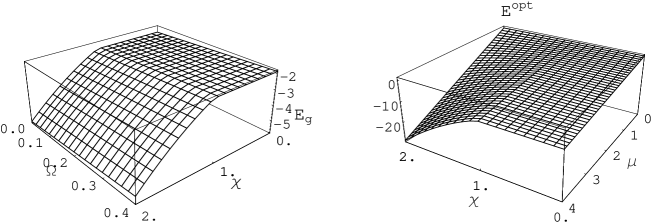
Figure 2: The ground state energy (4) in the $\chi$-$\Omega$ plane at $\mu=2.5$ (a) and in the plane $\chi-\mu$ ($\Omega=1$) (b). The seltrapping dominated phase at $\chi<1$ and the tunneling dominated phase at $\chi>1$.

The ground state energy, especially its behavior dependent on pairs of parameters $\chi$, $\Omega$ and $\chi$, $\mu$ is illustrated in details in Fig. 2. While being weakly $\Omega$-dependent, the energy strongly decreases with $\chi$ inside the ”light” phase (Fig. 2a). The position of the phase line is slightly shifted from $\chi=1$ at $\Omega=0$ to higher values of $\chi$ with increasing $\Omega$. This is consistent with the fact that the phonon fluctuations are most effective when the difference of the energies of the phases is of the order of the phonon energy.

The ground state energy in the ”heavy” region ($\chi<1$) is independent of $\chi$, its decrease inside the ”light” region ($\chi>1$) is dependent on the effective coupling $\mu$ (Fig. 2b). The energy decrease due to $\mu$ is stronger in the ”light” phase (depending on $\chi$) than in the ”heavy” phase.

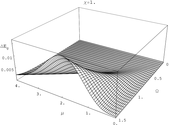
Figure 3: The range of relevance of the reflection parameter $\eta$: Difference $\Delta E_{G}=E_{G}(\eta=0,r=0)-E_{G}$, for $\chi=1$, $E_{G}$ is the exact ground state (23). For $\chi<1$, the difference increases with $\chi$ reaching its maximum at $\chi=1$. At $\chi>1$ it drops to zero, i.e. the narrow minimum ”light” phase is resistant against $\eta$.

The region of importance of reflection measure $\eta$ and $r$ is illustrated in the Fig. 3. There we show the difference between the ground state energy with $r$ and $\eta$ omitted and ground state with four variational parameters calculated numerically. However, contribution due to $r$ $E_{G}(\eta,r=0)-E_{G}\sim 2.10^{-3}$ of the maximum value in Fig. 3. The said parameters turn out to be most relevant in E$\otimes$e JT case ($\chi=1$).

The effects of $\eta$ and $r$ on the ground state is apparent only at moderate couplings in the ”heavy” region, reaching their maximum at $\chi=1$. The narrow minimum (the ”light” region) is resistant against $\eta$.

In order to demonstrate important properties of displacements ($\mu$ and $\Omega$ dependence) it is sufficient, except of the region of importance of the reflection (Fig. 3) inside the ”heavy” region apparent for $\gamma_{2}$, to calculate them in the limit $\eta=0$. We shall use Eq. (22) approximated for the cases of both ”heavy” and ”light” polaron and obtain implicit expressions for $\gamma_{i}$ which however are good to visualize their behaviour in both regions:

(i) ”heavy” polaron ($\gamma_{2}$ small, $E_{2}\approx 1,H_{T_{2}},H_{T_{4}}\approx 0$):

$$\gamma_{1} \approx \frac{-\alpha e^{4r}}{2TE_{1}^{2}\left[2+\frac{\Omega e^{4r}}{TE_{1}^{2}}\right]},$$ (25)

$\gamma_{2}$ is small except of the region of fluctuations visualized in Fig. 4. One can see, that the selflocalization due to phonons $2$ in the ”heavy” region $\sim-\gamma_{2}^{2}$ clearly implies the ”cave” in the ground state energy due to the reflection measure $\eta$ (anharmonicity) of the ground state (Fig. 3).

(ii) ”light” polaron ($\gamma_{1}$ small, $E_{1}\approx 1,H_{T_{2}},H_{T_{3}}\approx 0$):

$$\gamma_{1} \approx \frac{-\alpha e^{4r}}{2TE_{1}^{2}\left(1+\frac{\beta^{2}}{2\Omega T}+\frac{\Omega e^{4r}}{TE_{1}^{2}}\right)}\approx 10^{-8},\quad\gamma_{2}\approx\frac{\beta}{2TE_{2}^{2}(2+\frac{\Omega}{TE_{2}^{2}})}.$$ (26)

In the ”light” region the fluctuations of $\gamma_{1}$ are missing as well as the fluctuations of the energy. This is consistent with the above result of the resistance of the narrow minimum against $\eta$.

For both ”heavy” and ”light” polaron a dependence of $\gamma_{i}$ on the nonadiabaticity parameter $\Omega/T$ appears. It implies the dependence of the Debye-Waller factor and consequently of the polaron mass on the phonon frequency $\Omega$. This can be thought of as an analogy of the isotope effect at zero temperature.

In the ”heavy” phase, electron transitions mediated by phonons $2$ to the upper level enhance fluctuations $\sim\gamma_{2}$ which mix phonons $2$ with phonons $1$ and contribute to the fluctuations of the ground state energy of the heavy region. This is the reason for the similarity of the results in Fig. 3.

4 Ground state of the local model

Now we consider the same Hamiltonian, but taken for the local molecule ($T=0$). From the outset we include the additional variational mixing parameter $\lambda$ into the Ansatz. The understanding of the importance of introducing the mixing parameter in the local model in the contrast to the lattice one can be gained if one examines the expressions for Hamiltonians, in particular, those terms which contain the mixing of two phonon modes. The mixing is contained mostly in the “local” term with $\beta$,

$$\beta Q_{2}\exp{i\pi(b_{1}^{+}b_{1})}.$$

The transfer term $T$ also contains the mixing, but it always enters the expression in the form $T(1+E_{1}E_{2})$, thus for the transfer term its contribution is always shadowed by the larger term $\sim 1$. Thus, if $T\neq 0$ and large enough, its contribution is always dominant over mixing term $\beta$. But if $T=0$, we are left with the only nonlinear coupling term $\beta Q_{2}\varepsilon$ and accurate accounting for mode mixing becomes crucial.

The variational mean value of the part of the Hamiltonian (6) in the state (9) renormalized by $\Omega$ yields (Appendix A)

$$\frac{\langle H\rangle}{\Omega}=\frac{1}{2}(\cosh 4r_{1}+\cosh 4r_{2})\cosh 2\lambda+(\zeta_{1}^{2}+\zeta_{2}^{2})$$

$$+\frac{2\eta}{C}\frac{\exp\left[-\frac{2\tilde{\zeta}_{1}^{2}}{\cosh 2\lambda}\right]}{\cosh 2\lambda}\left\{-\tanh 2\lambda\sinh 2\lambda\cosh 2(r_{1}+r_{2})\cosh 2(r_{1}-r_{2})\right.$$

$$\left.+\tilde{\zeta}_{1}^{2}[(\exp 2(r_{1}+r_{2})-\exp(-2(r_{1}+r_{2}))\cosh 4\lambda)(1+\tanh^{2}2\lambda)\right.$$

$$\left.+2\exp(-2(r_{1}+r_{2}))\sinh 4\lambda\tanh 2\lambda]\cosh 2(r_{1}-r_{2})\right.$$

$$\left.+\frac{\tilde{\zeta}_{1}^{2}}{\cosh^{2}2\lambda}(\sinh 4r_{1}-\sinh 4r_{2})-2\zeta_{1}(\tanh(2\lambda)e^{2(r_{2}-r_{1})}\zeta_{2}+\zeta_{1})\right\}$$ (27)

$$+\frac{2\alpha}{\Omega C}(1-\eta^{2})\zeta_{1}$$

$$-\frac{2\beta}{\Omega C}\left\{(1+\eta^{2})[\zeta_{2}-\zeta_{1}\tanh 2\lambda\exp 2(r_{2}-r_{1})]\frac{\exp\left(-\frac{2\tilde{\zeta}_{1}^{2}}{\cosh 2\lambda}\right)}{\cosh 2\lambda}+2\eta\zeta_{2}\right\}\,,$$

where

$$\tilde{\zeta}_{1}=\zeta_{1}\exp(-2r_{1}),\quad C=1+2\eta\frac{\exp(-\frac{2\tilde{\zeta}_{1}^{2}}{\cosh 2\lambda})}{\cosh 2\lambda}+\eta^{2}.$$ (28)

From Eq. (4) one can see that $\lambda$ causes correlations of the selftrapping and tunneling dominated regions.

For $\lambda=0$, Eq. (4) turns to

$$\frac{\langle H\rangle_{\lambda=0}}{\Omega}=\frac{1}{2}(\cosh 4r_{1}+\cosh 4r_{2})+\frac{1}{C_{0}}\left(1-2\eta e^{-8r_{1}}\exp(-2\tilde{\zeta}_{1}^{2})+\eta^{2}\right)\zeta_{1}^{2}$$

$$+\Omega\zeta_{2}^{2}+\frac{2\alpha}{\Omega C_{0}}(1-\eta^{2})\zeta_{1}-\frac{2\beta}{\Omega C_{0}}[(1+\eta^{2})\exp(-2\tilde{\zeta}_{1}^{2})+2\eta]\zeta_{2}$$ (29)

where

$$C_{0}=1+2\eta\exp(-2\tilde{\zeta}_{1}^{2})+\eta^{2}.$$ (30)

For $\eta=0$, $C=1$ and (4) becomes

$$\frac{\langle H\rangle_{\eta=0}}{\Omega}=\frac{1}{2}(\cosh 4r_{1}+\cosh 4r_{2})\cosh 2\lambda+\zeta_{1}^{2}+\zeta_{2}^{2}+\frac{2\alpha}{\Omega}\zeta_{1}$$

$$-\frac{2\beta}{\Omega}(\zeta_{2}-\zeta_{1}\tanh 2\lambda\exp 2(r_{2}-r_{1}))\frac{\exp\left(-\frac{2\tilde{\zeta}_{1}^{2}}{\cosh 2\lambda}\right)}{\cosh 2\lambda}$$ (31)

The ground states of (4), (29) and (31) were found by minimalization of the expressions against the involved VPs. The respective ground state energies $E^{opt}$, $E_{\lambda=0}^{opt}$, $E_{\eta=0}^{opt}$ and $E_{\eta=0,\lambda=0,opt}$ will be compared mutually and with the exact value from numerical simulation in order to find out importance of the variational parameters $\eta,\lambda$ in different regions of model parameters $\chi=\frac{\beta}{\alpha}$ (reflection) and $\mu=\frac{\alpha^{2}}{\Omega^{2}}$ (effective e-ph coupling). The place of E$\otimes$e JT model will clearly come out as an important special case.

5 Discussion of the numerical results

In lattice electron-phonon models the nonadiabaticity parameter is the ratio of phonon frequency and the band width, $\frac{\Omega}{T}$. The energy is scaled by $T$ and the effective coupling parameter (ratio of the polaron energy and of the phonon frequency) is $\mu_{T}=\alpha^{2}/2\Omega T$). In the present local model, the nonadiabaticity parameter is the ratio of the frequency and the coupling parameter $\Omega/\alpha$. The energy was scaled by $\Omega$ and the ratio of polaron energy and the frequency is then $\alpha^{2}/2\Omega^{2}$. Therefore, the reduction of the ground state energy of the local model due to selflocalization is stronger than that of the lattice model by the factor $\mu_{L}/\mu_{T}=T/\Omega>1$. The energy of the tunneling $\beta^{2}/\Omega^{2}$, is comparable with the polaron energy at $\beta^{2}/\Omega^{2}=\mu_{L}$. Because close to $\chi=1$ there is $\zeta_{1}\approx 0$, the effects of all variational parameters for $\chi>1$ except of $\zeta_{2}$ vanish. Quantum fluctuations due to $r_{1},r_{2}$ and anharmonicity due to $\lambda$ are concentrated in the crossing region close to $\mu=1$ and $\chi=1$.

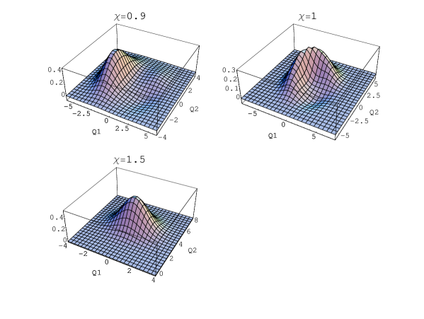
Figure 4: The numerical ground state wave functions at $\mu=2$ and $\chi=0.9$ (a) $\chi=1$ (b) and $\chi=1.5$ (c).

The ground state in the phase plane $\chi$ and $\mu$ shown in Fig.4 exhibits two phases separated by the crossover line close to $\chi=1$. It means, that the effective polaron potential exhibits two minima which reflect positions of two levels governed by the model parameters $\mu$ and $\chi$. The minima coincide within the border of the regions close to $\chi=1$. The phase $\chi<1$ is $\chi$ independent, selftrapping dominated, with quantum fluctuations due to $\lambda,\eta,r_{1},r_{2}$. The phase $\chi>1$ is the phonon-2-assisted tunneling dominated region with continuum emission and absorption of virtual phonons-$1$. The phonon exchange couples the levels within one minimum. The minimum is much more sensitive to the change of model parameters $\mu,\chi$ as well as to quantum fluctuations $r_{1},r_{2}$ and $\lambda$.

Electron in the selftrapping dominated region is trapped by the phonons-$1$ but due to the interactions mediated by phonons-2 the electron can fluctuate to the higher level. Due to the reflection symmetry of the phonons-2 continuum oscillations of the electrons at simultaneous emission and absorption of phonons-1 occurs. These oscillations couple the levels and so the electrons into pairs. This mechanism was described in a recent paper [10] for a lattice model.

From (31), for small $\chi$, one can approximately take $\zeta_{2}\approx 0$, $\zeta_{1}\approx-\frac{\alpha}{\Omega}$ and for $\lambda$ we are left with the result $\lambda\approx\mu\chi\exp(-2\mu)$. This dependence can be recognized in Fig.5.

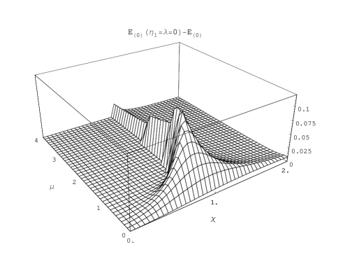
Figure 5: The difference of $E(\eta=0,\lambda_{opt})-E(\eta_{opt},\lambda_{opt})$.

Figure 6: The difference of $E(\eta=0,\lambda_{opt})-E(\eta_{opt},\lambda_{opt})$ including the mode correlation (a), without the correlation (b). Strong suppression of the reflection effects by the mode correlation at $\mu<1$ is evident. The correlations flatten the barrier between the zones and the role of the parameter $\eta$ is minorized (Note the difference of the scales of Figs. (a) and (b)).

Comparing Figs. 6a and 6b one can see that the mode correlation induced anharmonicity $\lambda$ (Fig.6a) is by one order larger than the contribution to the anharmonicity of the reflection level mixing $\eta$ Fig.6b. The correlation is most effective for weak effective couplings $\mu$ at $\chi\approx 1$. For large $\mu$ it contributes only close to $\chi=1$, where it reveals maximum for all $\mu$. In order to check the validity of the calculations using variational approach we performed also numerical diagonalization of the Hamiltonian in the phonon-$1,2$ space. We limit ourselves in $N_{1}$ phonon-1 states and $N_{2}$ phonon-2 states, thus state vector is $N_{1}\times N_{2}$ dimensional. As numerical diagonalization results show, about 20-50 phonon states are sufficient for convergence. We show the results of numerical diagonalization of Hamiltonian matrix as function of $\chi$ for $\mu=1$ and $\mu=4$. In the first case we took 20$\times$20 state vector, while in the latter case to achieve satisfactory convergence (especially for the tunneling-dominated region when $\chi>1$) we had to increase the number of phonons-2 up to 50.

6 Quantum fluctuations in the local model

Fluctuations of phonon-1 coordinate $\Delta Q_{1}^{2}=\langle Q_{1}^{2}\rangle-\langle Q_{1}\rangle^{2}$, $Q_{1}=\frac{1}{\sqrt{2}}(b_{1}^{{\dagger}}+b_{1})$ and the conjugate momentum $P_{1}=\frac{-i}{\sqrt{2}}(b_{1}^{{\dagger}}-b_{1})$ for $\eta=0$ can be easily calculated analytically. The wave function of the phonon-$1$ has the Gaussian form

$$\phi(x)\sim\exp\left[-\frac{(x-\lambda_{1})^{2}}{\cosh(2\lambda)\exp(4r_{1})}\right].$$

In fact, it is squeezed displaced harmonic oscillator if one does not take into account the parameter $\eta$; Introducing $\lambda$ does not invoke higher order nonlinearities with respect to phonon-$1$ coordinates. Thus $\langle\Delta P_{1}\rangle=0$, like it should be for an harmonic oscillator, and the expressions for second momenta have the form:

$$\Delta Q_{1}^{2}=\frac{1}{2}\exp 4r_{1}\cosh 2\lambda,\quad\Delta P_{1}^{2}=\frac{1}{2}\exp(-4r_{1})\cosh 2\lambda$$ (32)

and

$$\left(\Delta P_{1}^{2}\Delta Q_{1}^{2}\right)^{1/2}=\frac{1}{2}\cosh 2\lambda.$$ (33)

The shape of fluctuations due to the correlation $\lambda$ (33) closely follows the shape of the curve in Fig.7, having its maximum close to $\chi=1$ and $\mu\approx 1$.

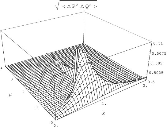
Figure 7: The product of uncertainties of the coordinate and the conjugated momentum of the phonon-$1$ for $\eta=0$.

The similarity of the product of uncertainties of phonon coordinate and momentum displayed in Fig.7. illustrates anharmonic source of the contribution due to the mode correlation. The correlations $\lambda$ manifest themselves in (32) and (33) as a phonon anharmonicity. It is noteworthy to emphasize its quantum origin (compare the note below Eq. (2)). The problem with $\eta\neq 0$ needs special consideration and will be considered elsewhere.

7 Conclusion

A suitable choice of the variational wave functions for various electron-phonon two-level systems is a long-standing problem in solid state physics as well as in quantum optics. For two-level reflection symmetric systems with intralevel electron-phonon interaction the approach with a variational two-center squeezed coherent phonon wave function was found to yield the lowest ground state energy. The two-center wave function was constructed as a linear combination of the phonon wave functions related to both levels introducing new VP.

This symmetry implies coupling of the levels mediated by continuous virtual emission and absorption of phonons accompanying the electron tunneling between the levels. This is an analogy of Rabi oscillations in quantum optics. Investigation of referring properties (tunneling rates, Debye-Waller factors) was performed mostly for the models with onsite (Holstein) electron-phonon interactions in dimer or exciton-phonon models and also for E$\otimes$e JT model. The methods used there were based on either combination of variational approach and unitary transformations or numerical diagonalization.

In two-level models with phonon assisted tunneling there appears coupling of both phonon modes mediated by Rabi oscillations. Therefore, also the interlevel quantum correlations of the phonons must be taken into account. This brings into the variational ansatz additional quantum VP.

The two-level system is characterized by strongly nonlinear effective potential provided by phonons. The nonlinearity is governed by the bare Hamiltonian parameters exhibiting a crossover from an asymmetric double potential well with two broad nonequivalent minima pertaining to the levels to a regime of one narrow minimum when the broad minima coincide into one potential well. This effect is due to the effective attraction of the levels by virtual exchange of phonons. Much effort was expended also to improve one-center variational approach by including correlations of the concerning two squeezed coherent phonon modes of the JT model. When compared to the lattice case, the local version of the model provides qualitatively similar effective potential. This conclusion was to be expected: in the symmetric case minima of the nonlinear effective potential related with two levels are close together and so the quantum fluctuations there are most effective. We considered both the mixing and squeezing correlation VP in order to find region of relevance of both parameters as functions of the interaction constants.

The support from the Grant Agency of the Czech Republic of our project No. 202/01/1450 is highly acknowledged. We thank also the grant agency VEGA (No. 2/7174/20) for partial support.

Appendix A

We used following formulas [11]

$$D_{1}(\eta_{1})S_{1}(r_{1})=S_{1}(r_{1})D_{1}(\tilde{\eta}_{1}),\ \tilde{\eta}_{1}=\eta_{1}e^{-2r}$$ (34)

$$S_{1}^{-1}(r_{1})b_{1}S_{1}(r_{1})=b_{1}\cosh 2r_{1}+b_{1}^{{\dagger}}\sinh 2r_{1}$$ (35)

$$S_{12}^{-1}(\lambda)b_{1}S_{12}(\lambda)=b_{1}\cosh\lambda+b_{2}^{{\dagger}}\sinh\lambda$$ (36)

$$\langle 0|S_{1}^{{\dagger}}(r)D_{1}^{{\dagger}}(\eta)\exp(\lambda b_{1}^{{\dagger}})\rangle=\frac{1}{(\cosh 2r)^{1/2}}$$

$$\times\exp\left[\frac{\lambda^{2}}{2}\tanh(2r)-\lambda\eta(\tanh 2r-1)-\frac{1}{2}\eta^{2}+\frac{1}{2}(\tanh 2r-1)\eta^{2}\right],$$ (37)

$$\langle 0|S_{1}(\zeta)D_{1}(\eta)b_{1}^{{\dagger}m}\rangle=\frac{d^{m}}{d\lambda^{m}}\langle 0|S_{1}(\zeta)D_{1}(\eta)\exp(\lambda b_{1}^{{\dagger}})\rangle|_{\lambda=0},$$ (38)

$$S_{12}(\lambda)=T^{{\dagger}}\left(\frac{\pi}{4}\right)S_{1}(\lambda/2)S_{2}(-\lambda/2)T\left(\frac{\pi}{4}\right)$$ (39)

$$T\left(\frac{\pi}{4}\right)\left(\matrix{b_{1}\cr b_{2}}\right)T^{{\dagger}}\left(\frac{\pi}{4}\right)=\frac{1}{\sqrt{2}}\left(\matrix{b_{1}-b_{2}\cr b_{1}+b_{2}}\right),$$ (40)

$$T^{{\dagger}}|0\rangle=T|0\rangle=|0\rangle$$ (41)

References

- [1] M. C. M. O’Brien and C. C. Chancey, Am.J.Phys. 61 (8), 688 (1993)
- [2] M. D. Kaplan and B. G. Vekhter, “Cooperative phenomena in Jahn-Teller crystals” (Ed. J. P. Fackler, Plenum, New York and London 1995).
- [3] O. Gunnarson, Phys. Rev. Lett. 74, 1875 (1995); O. Gunnarson, Rev. Mod. Phys. 69, 575 (1997).
- [4] H. B. Shore and L. M. Sander, Phys. Rev. B 7 (10), 4537 (1973)
- [5] M. Sonnek, T. Frank and M. Wagner, Phys. Rev. B 49 (22), 15637 (1994)
- [6] C.F. Lo, Phys. Rev. A 43 (9), 5127 (1991)
- [7] C.F. Lo and R. Sollie, Phys.Rev. B 44 (10), 5013 (1991)
- [8] R.L. Fulton and M. Gouterman, J. Chem. Phys. 35, 1059 (1961).
- [9] B. W. Shore, and P. L. Knight, J. Mod. Opt. 40, 1195 (1993); I.I. Rabi, Phys.Rev. 49, 324 (1936); Phys. Rev. 51, 652 (1937).
- [10] E. Majerníková, J. Riedel and S. Shpyrko, Phys. Rev. B 65 (17), 174305 (2002)
- [11] B. L. Schumaker, Phys. Repts. 133 (6), 317 (1986)