Applications of exact solution for strongly interacting one dimensional bose-fermi mixture: low-temperature correlation functions, density profiles and collective modes.

Abstract

We consider one dimensional interacting bose-fermi mixture with equal masses of bosons and fermions, and with equal and repulsive interactions between bose-fermi and bose-bose particles. Such a system can be realized in current experiments with ultracold bose-fermi mixtures. We apply the Bethe-ansatz technique to find the exact ground state energy at zero temperature for any value of interaction strength and density ratio between bosons and fermions. We use it to prove the absence of the demixing, contrary to prediction of a mean field approximation. Combining exact solution with local density approximation (LDA) in a harmonic trap, we calculate the density profiles and frequencies of collective modes in various limits. In the strongly interacting regime, we predict the appearance of low-lying collective oscillations which correspond to the counterflow of the two species. In the strongly interacting regime we use exact wavefunction to calculate the single particle correlation functions for bosons and fermions at low temperatures under periodic boundary conditions. Fourier transform of the correlation function is a momentum distribution, which can be measured in time-of-flight experiments or using Bragg scattering. We derive an analytical formula, which allows to calculate correlation functions at all distances numerically for a polynomial time in the system size. We investigate numerically two strong singularities of the momentum distribution for fermions at $k_{f}$ and $k_{f}+2k_{b}.$ We show, that in strongly interacting regime correlation functions change dramatically as temperature changes from $0$ to a small temperature $\sim E_{f}/\gamma\ll E_{f},$ where $E_{f}=(\pi\hbar n)^{2}/(2m),\;n$ is the total density and $\gamma=mg/(\hbar^{2}n)\gg 1$ is the Lieb-Liniger parameter. A strong change of the momentum distribution in a small range of temperatures can be used to perform a thermometry at very small temperatures.

I Introduction

Recent developments in cooling and trapping of cold atoms open exciting opportunities for experimental studies of interacting systems under well controlled conditions. Current experiments bfexp ; fermipressure can deal not only with single component gases, but with various atomic mixtures. Using FeshbachKRbFeshbach ; LiNaFeshbach resonances and and/or optical latticesJaksch98 ; Bloch one can tune different parameters, and drive the systems towards strongly correlated regime. The effect of correlations is most prominent for low dimensional systems, and recent experimental realizationWeiss ; Paredes of a strongly interacting Tonks-Girardeau (TG) gas of bosons opens new perspectives in experimental studies of strongly interacting systems in 1DMoritz1dmolecules . In this article we investigate bose-fermi mixtures in 1D, using exact techniques of the Bethe ansatz. Some of the results presented here have been reported earlier bfshort .

Most of the theoretical research on bose-fermi mixturesbftheory so far has been concentrated on higher dimensional systems, and only recently 1D systems started attracting attention. Several properties of such systems have been investigated so far, including phase separationDas ; CazalillaHo ; jap_numerics , fermion pairingMathey , possibility of charge density wave (CDW) formationCDW and long distance behavior of correlation functionsFrahm .

A 1D interacting bose-fermi mixture is described by the Hamiltonian

$$H=\int_{0}^{L}dx(\frac{\hbar^{2}}{2m_{b}}\partial_{x}\Psi_{b}^{\dagger}\partial_{x}\Psi_{b}+\frac{\hbar^{2}}{2m_{f}}\partial_{x}\Psi_{f}^{\dagger}\partial_{x}\Psi_{f})+\int_{0}^{L}dx(\frac{1}{2}g_{bb}\Psi_{b}^{\dagger}\Psi_{b}^{\dagger}\Psi_{b}\Psi_{b}+g_{bf}\Psi_{b}^{\dagger}\Psi_{f}^{\dagger}\Psi_{f}\Psi_{b}).$$ (1)

Here, $\Psi_{b},\Psi_{f}$ are boson and fermion operators, $m_{b},m_{f}$ are the masses, and $g_{bb},g_{bf}$ are bose-bose and bose-fermi interaction strengths. The model (1) is exactly solvable, whenLai

$$m_{f}=m_{b}=m,\,g_{bb}=g_{bf}=g>0.$$ (2)

It corresponds to the situation when masses are the same, and bose-bose and bose-fermi interaction strengths are the same and positive. Although conditions (2) are somewhat restrictive, the exactly solvable case is relevant to current experiments (the experimental situation will be analyzed in detail in section VII ) and can be used to check the validity of different approximate approaches. Model (1) under conditions (2) has been considered in the literature beforeLai , but its properties have not been investigated in detail. After the appearance of our initial report bfshort , two additional articles Frahm ; Batchelor used Bethe ansatz to investigate the same model. We use the exact solution to calculate the ground state energy and investigate phase separation and collective modes at zero temperature. For strongly interacting regime, we calculate single particle correlation functions, and consider the effects of small temperature on correlation functions and density profiles.

The article is organized as follows. In section II we review the Bethe ansatz solution for bose-fermi mixture and compare it to the solution for fermi mixture. In section III we obtain the energy numerically in the thermodynamic limit. We use it to prove the absence of the demixing under conditions (2), contrary to prediction of a mean field Das approximation. In section IV we combine exact solution with local density approximation (LDA) in a harmonic trap, and calculate the density profiles and frequencies of collective modes in various limits. In the strongly interacting regime, we predict the appearance of low-lying collective oscillations which correspond to the counterflow of the two species. In section V we use exact wavefunction in the strongly interacting regime to calculate the single particle correlation functions for bosons and fermions at zero temperature under periodic boundary conditions. We derive an analytical formula, which allows to calculate correlation functions at all distances numerically for a polynomial time in system size. In section VI we extend the results of section V for low temperatures. We also calculate the evolution of the zero temperature density profile at small nonzero temperatures. We show, that in strongly interacting regime correlation functions change dramatically as temperature is raised from $0$ to a small value. Finally in section VII we analyze the experimental situation and make concluding remarks.

II Bethe ansatz solution

In this section we will briefly review the solution Lai of the model (1) under periodic boundary conditions and compare it to the solution of Yang of the spin-$\frac{1}{2}$ interacting fermions Yang67 ; Gaudin , for the sake of completeness. More details on Yang’s solution can be found in babooks ; takahashi ; Tsvelick ; Andrei ; Sutherlandbook .

In first quantization, hamiltonian (1) can be written as

$$H=-\sum_{i=1}^{N}\frac{\partial^{2}}{\partial x_{i}^{2}}+2c\sum_{i<j}\delta(x_{i}-x_{j}),\;c>0.$$ (3)

Here we have assumed $m=1/2$ and $\hbar=1,$ to keep contact with the literature on the subject. Later in the discussion of the collective modes we will introduce the mass of atoms, but it should be clear from the context whether we have assumed $m=1/2$ or not. $c$ in (3) is connected to parameters of (1) via

$$c=\frac{mg}{\hbar^{2}}.$$ (4)

Wave function is supposed to be symmetric with respect to indices $i=\{1,...,M\}$ (bosons) and antisymmetric with respect to $i=\{M+1,...,N\}$ (fermions). On the first stage, Yang’s solution doesn’t impose any symmetry constraint on the wavefunction. On the second stage, periodic boundary conditions are resolved with the help of extra Bethe-ansatz. This idea has been generalized by Sutherland Sutherland68 for the case of N-fermion species. The results presented here can be simply derived from Sutherland’s work.

In Yang’s solution, one assumes the generalized coordinate Bethe wavefunction of the following form: for $0<x_{Q_{1}}<x_{Q_{2}}<...<x_{Q_{N}}<L$

$$\Psi=\sum_{P}[Q,P]e^{i\sum{k_{P_{i}}x_{Q_{i}}}},E=\sum_{i}k^{2}_{i}.$$ (5)

where $k_{1},...,k_{N}$ is a set of unequal numbers, $P$ is an arbitrary permutation from $S_{N}$ and $[Q,P]$ is $N!\times N!$ matrix. Let’s denote the columns of this matrix as $N!$ dimensional vector $\xi_{P}.$ Delta function potential in (3) is equivalent to the following boundary condition for the derivatives of the wavefunction:

$$(\frac{\partial}{\partial x_{j}}-\frac{\partial}{\partial x_{k}})\Psi_{x_{j}=x_{k}+0}-(\frac{\partial}{\partial x_{j}}-\frac{\partial}{\partial x_{k}})\Psi_{x_{j}=x_{k}-0}=2c\Psi_{x_{j}=x_{k}},$$ (6)

and the continuity condition reads

$$\Psi_{x_{j}=x_{k}+0}=\Psi_{x_{j}=x_{k}-0}.$$ (7)

Suppose $Q$ and $Q^{\prime}$ are two permutations, such that $Q_{k}=Q^{\prime}_{k},$ for $k\neq\{i,i+1\},$ and $Q_{i}=Q^{\prime}_{i+1},Q^{\prime}_{i}=Q_{i+1}.$ Similarly, $P$ and $P^{\prime}$ are two permutations, such that $P_{k}=P^{\prime}_{k},$ for $k\neq\{i,i+1\},$ and $P_{i}=P^{\prime}_{i+1},P^{\prime}_{i}=P_{i+1}.$ To satisfy (6) and (7) for $x_{Q_{i}}=x_{Q_{i+1}}$ independently of other $x,$ one has to impose two conditions for four coefficients $[Q,P],[Q^{\prime},P],[Q,P^{\prime}],[Q^{\prime},P^{\prime}].$ Using these two conditions, we can express $[Q,P^{\prime}],[Q^{\prime},P^{\prime}]$ via $[Q,P],[Q^{\prime},P].$ These requirements can be simply written as a condition between $\xi_{P}$ and $\xi_{P^{\prime}}:$

$$\xi_{P^{\prime}}=Y^{i,i+1}_{P_{i},P_{i+1}}\xi_{P}.$$ (8)

$Y$ operators are defined as

$$Y^{l,m}_{i,j}=-\frac{\lambda_{ij}}{1+\lambda_{ij}}+\frac{1}{1+\lambda_{ij}}\hat{P}_{lm},$$ (9)

where

$$\lambda_{ij}=\frac{ic}{k_{i}-k_{j}},$$

and $\hat{P}_{lm}$ is an operator acting on a vector $\xi_{P}$ which interchanges the elements with indices $Q_{l}$ and $Q_{m}.$ Using $Y$ operators one can express any $\xi_{P}$ via $\xi_{0},$ where $\xi_{0}$ is a column for $P=$ identity. However, arbitrary permutation $P$ can be represented as a combination of neighboring transpositions by different means. Independence of the final result on a particular choice of neighboring transpositions can be checked based on the following Yang-Baxter Relations:

$$Y^{a,b}_{i,j}Y^{a,b}_{j,i}=1,$$ (10)

$$Y^{a,b}_{j,k}Y^{b,c}_{i,k}Y^{a,b}_{i,j}=Y^{b,c}_{i,j}Y^{a,b}_{i,k}Y^{b,c}_{j,k}.$$ (11)

Operators $Y^{i,i+1}_{P_{i},P_{i+1}}$ exchange the momentum labels $P_{i}$ and $P_{i+1},$ while $\hat{P}_{i,i+1}$ interchange relative position labels $Q_{i}$ and $Q_{i+1}$. It is convenient to define combined operator, which exchanges both labels:

$$X_{ij}=\hat{P}_{ij}Y^{ij}_{ij}=\frac{1-\lambda_{ij}\hat{P}_{ij}}{1+\lambda_{ij}}.$$ (12)

Using this definition, periodic boundary conditions can be written as $N$ matrix eigenvalue equations:

$$X_{j+1,j}X_{j+2,j}...X_{N,j}X_{1,j}...X_{j-1,j}\xi_{0}=e^{ik_{j}L}\xi_{0}.$$ (13)

The procedure outlined above reduces equations for $N!\times N!$ coefficients to $N$ eigenvalue equations for $N!$ dimensional vector. Imposing some symmetry on $\xi_{0}$ simplifies the system further. If $\xi_{0}$ is antisymmetric with respect to particle permutations (fermions) , then $\hat{P}_{ij}=-1$ and $e^{ik_{j}L}=1.$ The system of equations is the same as for noninteracting fermions, as expected. If $\xi_{0}$ is symmetric (bosons), $\hat{P}_{ij}=1$ and the system is equivalent to periodic boundary conditions of Lieb-Liniger model LL .

If one needs to consider two-species system, $\xi_{0}$ has the symmetry of the corresponding permutation group representation (Young tableau). Instead of solving eq. (13), it is convenient to consider the similar problem in the conjugate representation. If $\xi_{0}$ is antisymmetric with respect to both permutations of the first $M$ indices and the rest $N-M$ (two-species fermions), eigenstate in conjugate representation $\varphi$ is symmetric with respect to first $M$ indices and is also symmetric with respect to permutations of the rest $N-M$ indices. Similarly, in conjugate representation for bose-fermi mixture with $M$ bosons and $N-M$ fermions $\varphi$ should be chosen to be antisymmetric for permutations of $M$ boson indices and symmetric with respect to permutations of $N-M$ fermion indices. The periodic boundary conditions are (note the change of the sign in the definition of $X^{\prime}_{ij}$ compared to $X_{ij}$):

$$X^{\prime}_{j+1,j}X^{\prime}_{j+2,j}...X^{\prime}_{N,j}X^{\prime}_{1,j}...X^{\prime}_{j-1,j}\varphi=e^{ik_{j}L}\varphi,$$ (14)

$$X^{\prime}_{ij}=\frac{1+\lambda_{ij}\hat{P}_{ij}}{1+\lambda_{ij}}.$$ (15)

Since $N!$-dimensional vector $\varphi$ has symmetry constraints, it has $C^{M}_{N}$ inequivalent components, characterized by the positions $y_{i}$ of $M$ spin-down fermions (or $M$ bosons respectively). One can think of the components of the vector $\varphi$ as of the values of the spin wavefunction, defined on an auxiliary one-dimensional lattice of size $N.$ $C^{M}_{N}$ independent values of $\varphi$ correspond to $C^{M}_{N}$ values of the wavefunction of $M$ ”particles” with coordinates $y_{i},$ living on this auxiliary lattice (since $\varphi$ is symmetric for $N-M$ fermion indices, these are considered to be vacancies). Wavefunction should be symmetric with respect to exchange of two ”particles” for two-species fermions, and antisymmetric for the case of bose-fermi mixture. To preserve the terminology of the two-species fermion solution for the case of bose-fermi mixture, later in the text we will always refer to the wavefunction on an auxiliary lattice as to ”spin” wavefunction, although it has a direct meaning only for two-species fermion case.

First, one can solve the problem for $M=1$McGuire . In this case there is no difference between two-species fermions or bose-fermi mixture. It can be shown (detailed derivations are available in the appendix of Andrei ), that in this case wavefunction in conjugate representation is

$$\varphi(M=1)=F(\Lambda,y)=\prod_{j=1}^{y-1}\frac{k_{j}-\Lambda+ic/2}{{k_{j+1}-\Lambda-ic/2}},$$ (16)

where new spectral parameter $\Lambda$ satisfies the following equation:

$$\prod_{i=1}^{N}\frac{k_{i}-\Lambda+ic/2}{k_{i}-\Lambda-ic/2}=1.$$ (17)

Periodic boundary conditions simplify to

$$e^{ik_{j}L}=\frac{k_{j}-\Lambda+ic/2}{k_{j}-\Lambda-ic/2},j=\{1,...,N\}$$ (18)

In an auxiliary lattice the wavefunction of one spin-deviate (or boson) $F(\Lambda,y)$ plays the role similar to one-particle basis function $e^{ikx}$ of the original coordinate Bethe ansatz, spectral parameter $\Lambda$ being the analog of the momentum $k.$

In the case when $M>1,$ Yang suggested that the solution of eqs. (14)-(15) again has the form of Bethe ansatz in the ”spin” subspace: for $1\leq y_{1}<y_{2}<...<y_{M}\leq N$

$$\varphi=\sum_{R}A(R)\prod_{i=1}^{M}F(\Lambda_{R_{i}},y_{i}),$$ (19)

where $\Lambda_{1},...,\Lambda_{M}$ is a set of unequal numbers, $R$ is an arbitrary permutation from $S_{M}.$ It can be shown Yang67 ; Andrei , that this ansatz solves (14)-(15) for two-species fermion system, if

$$\frac{A(R^{\prime})}{A(R)}=\frac{\Lambda_{R_{i+1}}-\Lambda_{R_{i}}-ic}{\Lambda_{R_{i+1}}-\Lambda_{R_{i}}+ic},$$ (20)

similarly to bosonic relations of Lieb-Liniger modelLL . Here $R$ and $R^{\prime}$ are two permutations from $S_{M}$ such that $R_{k}=R^{\prime}_{k},$ for $k\neq\{i,i+1\},$ and $R_{i}=R^{\prime}_{i+1},R^{\prime}_{i}=R_{i+1}.$ The set of $\Lambda,k$ has to satisfy the following set of equations:

$$-\prod_{i=1}^{N}\frac{k_{i}-\Lambda_{\alpha}+ic/2}{k_{i}-\Lambda_{\alpha}-ic/2}=\prod_{\beta=1}^{M}\frac{\Lambda_{\beta}-\Lambda_{\alpha}+ic}{\Lambda_{\beta}-\Lambda_{\alpha}-ic},\alpha=\{1,...,M\},$$ (21)

$$e^{ik_{j}L}=\prod_{\beta=1}^{M}\frac{k_{j}-\Lambda_{\beta}+ic/2}{k_{j}-\Lambda_{\beta}-ic/2},j=\{1,...,N\}.$$ (22)

For the bose-fermi mixture, $\varphi$ has to be antisymmetric for permutations of $y_{i}$ variables. This problem has actually been solved by SutherlandSutherland68 , although he was interested not in bose-fermi mixture, but fermion model with several species. He has shown, that if one doesn’t specify the symmetry of $\varphi$ for $y_{i}$ variables and applies the generalized ansatz

$$\varphi=\sum_{R}[G,R]\prod_{i=1}^{M}F(\Lambda_{R_{i}},y_{G_{i}})$$ (23)

for $1\leq y_{G_{1}}<y_{G_{2}}<...<y_{G_{M}}\leq N$, then columns of $M!\times M!$ dimensional matrix $[G,R]$ are related similarly to (8):

$$\xi_{R^{\prime}}=Y^{\prime i,i+1}_{R_{i},R_{i+1}}\xi_{R}.$$ (24)

$Y^{\prime}$ operators are defined as

$$Y^{\prime l,m}_{i,j}=\frac{\kappa_{ij}+\hat{P}_{lm}}{1-\kappa_{ij}},\kappa_{ij}=\frac{ic}{\Lambda_{i}-\Lambda_{j}}.$$ (25)

For two-species fermions in conjugate representation $\hat{P}_{lm}=1,$ and it is equivalent to (20), while for bose-fermi mixture in conjugate representation $\hat{P}_{lm}=-1,$ and the answer is much more simple:

$$Y^{\prime l,m}_{i,j}=-1.$$ (26)

Therefore, ”spin” part of wavefunction is constructed by total antisymmetrization of single ”spin” wavefunctions, similar to Slater determinant for fermionic particles:

$$\varphi=\det(F(\Lambda_{i},y_{j})).$$ (27)

Periodic boundary conditions for bose-fermi mixture are:

$$\prod_{i=1}^{N}\frac{k_{i}-\Lambda_{\alpha}+ic/2}{k_{i}-\Lambda_{\alpha}-ic/2}=1,\alpha=\{1,...,M\},$$ (28)

$$e^{ik_{j}L}=\prod_{\beta=1}^{M}\frac{k_{j}-\Lambda_{\beta}+ic/2}{k_{j}-\Lambda_{\beta}-ic/2},j=\{1,...,N\}.$$ (29)

One can prove that all solutions of (28)-(29) are always real, which is a major simplification for the analysis of both ground and excited states (see Appendix A).

If one introduces function

$$\theta(k)=-2\tan^{-1}(k/c),$$ (30)

the system (28)-(29) can be rewritten as

$$k_{j}L=2\pi I_{j}+\sum_{\beta=1}^{M}\theta(2k_{j}-2\Lambda_{\beta}),$$ (31)

$$2\pi I_{\alpha}=\sum_{j=1}^{N}\theta(2\Lambda_{\alpha}-2k_{j}).$$ (32)

$I_{j}$ and $I_{\alpha}$ are integer or half integer quantum numbers (depending on the parity of M and N), which characterize the state. The ground state corresponds to

$$I_{\alpha}=(M-1)/2,-(M-3)/2,....,(M-1)/2\},$$ (33)

$$I_{j}=\{-(N-1)/2,-(N-3)/2,....,(N-1)/2\}.$$ (34)

In the thermodynamic limit, one has to send $M,N,L$ to infinity proportionally. If one introduces density of $k$ roots $\rho(k)$ and density of $\Lambda$ roots $\sigma(\Lambda),$ (28)-(29) simplifies to two coupled integral equations

$$2\pi\rho(k)=1+\int_{-B}^{B}\frac{4c\sigma(\Lambda)d\Lambda}{c^{2}+4(\Lambda-k)^{2}},$$ (35)

$$2\pi\sigma(\Lambda)=\int_{-Q}^{Q}\frac{4c\rho(\omega)d\omega}{c^{2}+4(\Lambda-\omega)^{2}}.$$ (36)

Normalization conditions and energy are given by

$$N/L=\int_{-Q}^{Q}\rho(k)dk,$$ (37)

$$M/L=\int_{-B}^{B}\sigma(\Lambda)d\Lambda,$$ (38)

$$E/L=\int_{-Q}^{Q}k^{2}\rho(k)dk.$$ (39)

These equations can be solved numerically and the results will be presented in the next section. Numerical solution of these equations allows to investigate the possibility of phase separation, predicted in Das . Combined with local density approximation, it can be used to investigate density profiles and collective oscillation modes in the external fields.

III Numerical Solution and Analysis of Instabilities

In this section we will solve the system of equations (35)-(39) numerically, and obtain the ground state energy as a function of interaction strength and densities. This solution will be used to analyze the instability towards demixingCazalillaHo ; Das ; jap_numerics .

Substituting (36) into (35), and performing analytically integration over $\Lambda,$ one obtains an integral equation for function $\rho(k).$ Similarly to LL , it is convenient to redefine the variables before solving this equation numerically. Let’s introduce the following variables $\lambda,x,y,b$ and a function $g(x)$ according to

$$c=\lambda Q,\omega=xQ,k=yQ,B=bQ,\rho(Qx)=g(x).$$ (40)

In new variables, integral equation depends on two parameters $b$ and $\lambda:$

$$2\pi g(y)=1+\int_{-1}^{1}\frac{2\lambda g(x)dx}{2\pi(\lambda^{2}+(x-y)^{2})}(\tan^{-1}{\frac{2(b-y)}{\lambda}}+\tan^{-1}{\frac{2(b-x)}{\lambda}}+$$

$$\tan^{-1}{\frac{2(b+y)}{\lambda}}+\tan^{-1}{\frac{2(b+x)}{\lambda}}+\frac{\lambda}{2(x-y)}\log{\frac{\lambda^{2}+4(b-x)^{2}}{\lambda^{2}+4(b-y)^{2}}\frac{\lambda^{2}+4(b+y)^{2}}{\lambda^{2}+4(b+x)^{2}}}).$$ (41)

In new variables, (37)-(39) become

$$\gamma=\frac{cL}{N}=\frac{\lambda}{\int_{-1}^{1}g(x)dx},$$ (42)

$$\frac{M}{N}=\frac{\int_{-1}^{1}(\tan^{-1}{\frac{2(b-x)}{\lambda}}+\tan^{-1}{\frac{2(b+x)}{\lambda}})g(x)dx}{\pi\int_{-1}^{1}g(x)dx},$$ (43)

$$E=\frac{N^{3}}{L^{2}}e(\lambda,b)=\frac{N^{3}}{L^{2}}\frac{\int_{-1}^{1}x^{2}g(x)dx}{\left(\int_{-1}^{1}g(x)dx\right)^{3}}.$$ (44)

Integral equation (41) can be solved numerically as a function of two parameters $b$ and $\lambda,$ applying Simpson rule for an integral approximation on a grid $x_{i}=-1+(i-1)/n,i=\{1,...,2n+1\}$. This gives a system of $2n+1$ linear equations for discrete values $g(x_{i}),$ which can be solved by standard methods. Using (42)-(44), one can obtain parametrically three functions $\gamma(\lambda,b),M/N=\alpha(\lambda,b),e(\lambda,b).$ After that one can numerically inverse two of them $\lambda(\gamma,\alpha)$ and $b(\gamma,\alpha),$ and obtain function $e(\gamma,\alpha).$ Resulting function is shown in fig. 1. When $\alpha=0,$ system is purely fermionic, and noninteracting. When $\alpha=1,$ the system is purely bosonic, and numerically obtained energy coincides with the result of LL . If $\gamma=0,$ bosons and fermions don’t interact, and $e(\gamma,\alpha)=(\pi^{2}/3)(1-\alpha)^{3}.$

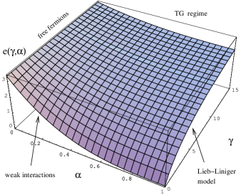
Figure 1: Energy of the ground state is given by $E=e(\gamma,\alpha)\hbar^{2}N^{3}/(2mL^{2}),$ where $\gamma=mg/(\hbar^{2}n),$ and $\alpha=M/N$ is the boson fraction. When $\alpha=0,$ system is purely fermionic, and the energy doesn’t depend on interactions. When $\alpha=1,$ the system is purely bosonic, and numerically obtained energy coincides with the result of LL . If $\gamma=0,$ bosons and fermions don’t interact, and $e(\gamma,\alpha)=(\pi^{2}/3)(1-\alpha)^{3}.$

An interesting case, where one can analytically find the dependence of energies on relative densities is Tonks-Girardeau (TG) regime of strong interactions, $\gamma\gg 1.$ In (41) one can neglect the dependence of the kernel on $x$ and $y,$ and $g(x)$ becomes a constant $g,$ which satisfies an equation

$$2\pi g=1+\frac{8g}{\pi\lambda}\left(\tan^{-1}{\frac{2b}{\lambda}}+\frac{2b\lambda}{\lambda^{2}+4b^{2}}\right),$$ (45)

while (43) reads

$$\alpha=\frac{2}{\pi}\tan^{-1}{\frac{2b}{\lambda}}.$$ (46)

After some algebra energy is rewritten as

$$e(\gamma,\alpha)=\frac{\pi^{2}}{3}\left(1-\frac{4}{\gamma}(\alpha+\frac{\sin{\pi\alpha}}{\pi})+\frac{12}{\gamma^{2}}(\alpha+\frac{\sin{\pi\alpha}}{\pi})^{2}\right)+O(\frac{1}{\gamma^{3}}).$$ (47)

Using exact solutions, one can analyze demixing instabilitiesCazalillaHo ; Das ; jap_numerics for repulsive bose-fermi mixtures. In the absence of external potential bose-fermi mixture is stable, if the compressibility matrix

$$\left[\begin{array}[]{cc}\frac{\partial\mu_{b}}{\partial{n_{b}}}&\frac{\partial\mu_{b}}{\partial{n_{f}}}\\ \frac{\partial\mu_{f}}{\partial{n_{b}}}&\frac{\partial\mu_{f}}{\partial{n_{f}}}\end{array}\right]$$ (48)

is positively defined. Here, $n_{b}$ is the boson density, and $n_{f}$ is the fermion density. $\mu_{b}$ and $\mu_{f}$ are the bose and fermi chemical potentials, given by

$$\mu_{b}=\frac{N^{2}}{L^{2}}\left(3e(\gamma,\alpha)-\gamma\frac{\partial e}{\partial\gamma}+(1-\alpha)\frac{\partial e}{\partial\alpha}\right),$$ (49)

$$\mu_{f}=\frac{N^{2}}{L^{2}}\left(3e(\gamma,\alpha)-\gamma\frac{\partial e}{\partial\gamma}-\alpha\frac{\partial e}{\partial\alpha}\right).$$ (50)

The fact that the matrix (48) is positively defined can be checked numerically for any value of $\alpha$ and $\gamma$, and proves that bose-fermi mixture with the same bose-fermi and bose-bose interactions is stable with respect to demixing for any values of bose and fermi densities. We note, that the absence of demixing for one particular value of the density has been checked in the original article by Lai and YangLai . Although an exact solution is available only under conditions (2), small deviations from these should not dramatically change the energy $e(\gamma,\alpha).$ Therefore, we expect the 1D mixtures to remain stable to demixing in the vicinity of the integrable line (2) for any interaction strength. Recently this has been checked numerically in Quantum Monte Carlo studies for a systems of up to $14$ atomsjap_numerics .

Note, that prediction of Das about demixing at sufficiently strong interactions in this case is incorrect, since it is based on the mean field approximation. Indeed, the demixing condition there reads

$$n_{f}\leq\frac{m_{f}g_{bf}^{2}}{g_{bb}\hbar^{2}\pi^{2}}.$$ (51)

For $g_{bf}=g_{bb}$ and $n_{b}=n_{f}$ it is equivalent to

$$\gamma=\frac{mg}{\hbar^{2}n}\geq\frac{\pi^{2}}{2}\approx 4.9.$$ (52)

Clearly, this condition is incompatible with mean-field approximation, which is valid for $\gamma\lesssim 1.$

For weakly interacting case one can use mean field approximation to calculate energy and chemical potentialsDas ; Batchelor :

$$E=L\left[\frac{g}{2}n_{b}^{2}+gn_{b}n_{f}+\frac{\hbar^{2}\pi^{2}}{2m}\frac{n_{f}^{3}}{3}\right],$$

$$\mu_{b}=g(n_{b}+n_{f}),\;\mu_{f}=gn_{b}+\frac{\hbar^{2}\pi^{2}}{2m}n_{f}^{2}.$$ (53)

For the strong interactions, up to corrections of order $1/\gamma^{3}$,

$$E=L\left[\frac{\hbar^{2}\pi^{2}}{2m}\frac{(n_{f}+n_{b})^{3}}{3}\right]\left(1-\frac{4}{\gamma}(\alpha+\frac{\sin{\pi\alpha}}{\pi})+\frac{12}{\gamma^{2}}(\alpha+\frac{\sin{\pi\alpha}}{\pi})^{2}\right),$$ (54)

$$\mu_{f}=\frac{\hbar^{2}\pi^{2}}{2m}(n_{f}+n_{b})^{2}(1+\frac{1}{3\gamma}\left(-16(\alpha+\frac{\sin{\pi\alpha}}{\pi})+4\alpha(1+\cos{\pi\alpha})\right)+$$

$$+\frac{1}{\gamma^{2}}(\alpha+\frac{\sin{\pi\alpha}}{\pi})\left(20(\alpha+\frac{\sin{\pi\alpha}}{\pi})-8\alpha(1+\cos{\pi\alpha})\right)),$$ (55)

$$\mu_{b}=\frac{\hbar^{2}\pi^{2}}{2m}(n_{f}+n_{b})^{2}(1+\frac{1}{3\gamma}\left(-16(\alpha+\frac{\sin{\pi\alpha}}{\pi})+4(\alpha-1)(1+\cos{\pi\alpha})\right)+$$

$$+\frac{1}{\gamma^{2}}(\alpha+\frac{\sin{\pi\alpha}}{\pi})\left(20(\alpha+\frac{\sin{\pi\alpha}}{\pi})+8(1-\alpha)(1+\cos{\pi\alpha})\right)).$$ (56)

IV Local density approximation and collective modes

So far our arguments have been limited to the case of periodic boundary conditions without external confinement. This is the situation, when the many-body interacting model (1) is exactly solvable in the mathematical sense. If one adds an external harmonic potential, model is not solvable any more. However, if external potential varies slowly enough (precise conditions for the case of bose gas have been formulated in ShlyapnikovLDA ), one can safely use local density approximation (LDA) to analyze the density profiles and collective modes in a harmonic trap. In the local density approximation, one assumes that in slowly varying external harmonic trap chemical potential changes according to

$$\mu^{0}_{b}(x)+\frac{m\omega^{2}_{b}x^{2}}{2}=\mu^{0}_{b}(0),\;\mu^{0}_{f}(x)+\frac{m\omega^{2}_{f}x^{2}}{2}=\mu^{0}_{f}(0).$$ (57)

Let us consider the case when external harmonic confining potential oscillator frequencies are the same for bosons and fermions. We note, however, that one can also analyze the case when $\omega_{b}\neq\omega_{f}$ in a similar way. We consider

$$\omega_{b}=\omega_{f}=\omega_{0},$$ (58)

since in this case distribution of the relative boson and fermion densities is controlled only by interactions, and not by external potential, since external potential couples only to total density. Eqs. (57) for $\omega_{b}=\omega_{f}=\omega_{0}$ imply that densities of bosons and fermions in the region where bosons and fermions coexist are governed by

$$\mu^{0}_{f}(x)+\frac{m\omega^{2}_{0}x^{2}}{2}=\mu^{0}_{f}(0),\;\mu^{0}_{b}(x)-\mu^{0}_{f}(x)=(n_{f}+n_{b})^{2}\frac{\partial e}{\partial\alpha}=\mu^{0}_{b}(0)-\mu^{0}_{f}(0).$$ (59)

One can show, that these equations cannot be simultaneously satisfied for the whole cloud, and the mixture phase separates in an external potential given by (58). For both strong and weak interactions bosons and fermions coexist in the central part, but the outer sections consist of Fermi gas only. In the weakly interacting limit, this can be interpreted as an effect of the Fermi pressurefermipressure : while bosons can condense to the center of the trap, Pauli principle pushes fermions apart. As interactions get stronger, the relative distribution of bosons and fermions changes, and Figs. 2 and 3 contrast the limits of strong and weak interactions. For strong interactions, the fermi density shows strong non-monotonous behavior.

When interactions are small Eqs. (53) and (59) imply that in the region of coexistence densities are given by

$$n^{0}_{b}(x)=n^{0}_{b}(0)(1-\frac{x^{2}}{x_{b}^{2}}),\;n^{0}_{f}(x)=n^{0}_{f}(0),\;\mbox{for}\;x^{2}<x_{b}^{2}.$$ (60)

Outside of the region of coexistence, density of fermions decays as the square root of inverse parabola:

$$n^{0}_{b}(x)=0,\;n^{0}_{f}(x)=\frac{n^{0}_{f}(0)}{\sqrt{1-\frac{x_{b}^{2}}{x_{f}^{2}}}}\sqrt{1-\frac{x^{2}}{x_{f}^{2}}},\;\mbox{for}\;x_{b}^{2}<x^{2}<x_{f}^{2}.$$ (61)

Parameters $x_{f}$ and $x_{b}$ are given by

$$x_{b}^{2}=\frac{2gn^{0}_{b}(0)}{m\omega_{0}^{2}},\;x_{f}^{2}=x_{b}^{2}+\frac{(\hbar\pi n^{0}_{f}(0))^{2}}{(m\omega_{0})^{2}}.$$ (62)

A typical graph of density distribution for weakly interacting case is shown is shown in Fig. 2.

Figure 2: Densities of bose and fermi gases in weakly interacting regime at zero temperature. Lieb-Liniger parameter in the center of a trap is $\gamma_{0}=0.18,$ overall number of bosons equals number of fermions. Total density in the center of a trap is taken to be $1$.

If effective $\gamma_{0}$ is much bigger than $1$ in the center of a harmonic trap, the total density $n^{0}(x)$ follows Tonks-Girardeau density profile

$$n^{0}(x)=n^{0}(0)\sqrt{1-\frac{x^{2}}{x_{f}^{2}}}.$$ (63)

From Eqs. (47) and (59) distribution of $\alpha(x)$ is controlled by the following equation:

$$n^{0}(x)^{3}(1+\cos{(\pi\alpha(x))})=n^{0}(0)^{3}(1+\cos{(\pi\alpha(0))}).$$ (64)

Since $1+\cos{(\pi\alpha(x))}$ is bound and $n^{0}(x)$ goes to $0$ near the edges of the cloud, this equation can’t be satisfied for all $x^{2}<x_{f}^{2},$ which means that only fermions will be present at the edges of the cloud, similarly to weakly interacting regime. Density distribution for equal number of bosons and fermions is shown in Fig. 3. The form of the profile is universal, as long as $\gamma_{0}\gg 1$ and the temperature is zero. Evolution of this profile for nonzero temperatures is shown in figure 14.

Figure 3: Densities of bose and fermi gases in strongly interacting regime at zero temperature. Lieb-Liniger parameter in the center of a trap is $\gamma_{0}\gg 1,$ overall number of bosons equals number of fermions. Total density in the center of the trap is taken to be $1$.

Recent experimentsMoritz demonstrated that collective oscillations of 1D gas provide useful information about interactions in the system. Here we will numerically investigate collective modes of the system, by solving hydrodynamic equations of motion. These equations have to be solved with proper boundary conditions at the edge of the bosonic and fermionic clouds. Within the region of coexistence of bosons and fermions, such oscillations can be described by four hydrodynamic equationsMenotti

$$\frac{\partial}{\partial t}\delta n_{b}+\frac{\partial}{\partial x}(n_{b}v_{b})=0,$$ (65)

$$m\frac{\partial}{\partial t}\delta v_{b}+\frac{\partial}{\partial x}(\mu_{b}+V_{ext,b}+\frac{1}{2}mv_{b}^{2})=0,$$ (66)

$$\frac{\partial}{\partial t}\delta n_{f}+\frac{\partial}{\partial x}(n_{f}v_{f})=0,$$ (67)

$$m\frac{\partial}{\partial t}\delta v_{f}+\frac{\partial}{\partial x}(\mu_{f}+V_{ext,f}+\frac{1}{2}mv_{f}^{2})=0.$$ (68)

In certain cases, analytical solutions of hydrodynamic equations are availableStringari ; Menotti and provide the frequencies of collective modes. When an analytic solution is not available, the ”sum rule” approach has been usedStringari ; Menotti ; Astrakharchik ; bfsumrule to obtain an upper bound for the frequencies of collective excitations. The disadvantage of the latter approach is an ambiguity in the choice of multipole operator which excites a particular mode, especially for multicomponent systemsbfsumrule . Here we develop an efficient numerical procedure for solving hydrodynamical equations in 1D, which doesn’t involve additional ”sum rule” approximation.

While looking at low amplitude oscillations, it is sufficient to substitute

$$n_{b}(x,t)=n_{b}^{0}(x)+\delta n_{b}(x)e^{i\omega t},$$ (69)

$$n_{b}(x,t)v_{b}(x,t)=n^{0}_{b}(x)\delta v_{b}(x)e^{i\omega t},$$ (70)

$$n_{f}(x,t)=n_{f}^{0}(x)+\delta n_{f}(x)e^{i\omega t},$$ (71)

$$n_{f}(x,t)v_{f}(x,t)=n^{0}_{f}(x,t)\delta v_{f}(x)e^{i\omega t},$$ (72)

$$\mu_{b}+V_{ext,b}+\frac{1}{2}mv_{b}^{2}=const1+\delta\mu_{b}(x)e^{i\omega t}=const1+(\delta n_{b}(x)\frac{\partial\mu_{b}}{\partial n_{b}}+\delta n_{f}(x)\frac{\partial\mu_{b}}{\partial n_{b}})e^{i\omega t},$$ (73)

$$\mu_{f}+V_{ext,f}+\frac{1}{2}mv_{f}^{2}=const2+\delta\mu_{f}(x)e^{i\omega t}=const2+(\delta n_{b}(x)\frac{\partial\mu_{f}}{\partial n_{b}}+\delta n_{f}(x)\frac{\partial\mu_{f}}{\partial n_{f}})e^{i\omega t}.$$ (74)

Here, $n_{b}^{0}(x)$ and $n_{f}^{0}(x)$ are densities obtained within local density approximation. Linearized system of hydrodynamic equations can be written as:

$$-m\omega^{2}\left[\begin{array}[]{c}\delta n_{b}(x)\\ \delta n_{f}(x)\end{array}\right]=\nabla\left(\left[\begin{array}[]{cc}n^{0}_{b}(x)&0\\ 0&n^{0}_{f}(x)\end{array}\right]\nabla\left(\left[\begin{array}[]{cc}\frac{\partial\mu_{b}}{\partial{n_{b}}}&\frac{\partial\mu_{b}}{\partial{n_{f}}}\\ \frac{\partial\mu_{f}}{\partial{n_{b}}}&\frac{\partial\mu_{f}}{\partial{n_{f}}}\end{array}\right]\left[\begin{array}[]{c}\delta n_{b}(x)\\ \delta n_{f}(x)\end{array}\right]\right)\right).$$ (84)

For numerical solutions and boundary conditions it is more convenient to work with independent functions $\delta\mu_{b}(x),\delta\mu_{f}(x).$ System of equations becomes

$$-m\omega^{2}\left[\begin{array}[]{c}\delta\mu_{b}(x)\\ \delta\mu_{f}(x)\end{array}\right]=\left[\begin{array}[]{cc}\frac{\partial\mu_{b}}{\partial{n_{b}}}&\frac{\partial\mu_{b}}{\partial{n_{f}}}\\ \frac{\partial\mu_{f}}{\partial{n_{b}}}&\frac{\partial\mu_{f}}{\partial{n_{f}}}\end{array}\right]\nabla\left(\left[\begin{array}[]{cc}n^{0}_{b}(x)&0\\ 0&n^{0}_{f}(x)\end{array}\right]\nabla\left[\begin{array}[]{c}\delta\mu_{b}(x)\\ \delta\mu_{f}(x)\end{array}\right]\right).$$ (93)

Outside of the region of coexistence of bosons and fermions, $\delta\mu^{out}_{f}$ satisfies the following equation:

$$-m\omega^{2}\delta\mu^{out}_{f}=\frac{\partial\mu_{f}^{out}}{\partial{n_{f}}}\nabla\left[n^{out}_{f}(x)\nabla\delta\mu^{out}_{f}\right].$$ (94)

All modes can be classified by their parity with respect to $x\rightarrow-x$ substitution, and will be investigated by parity-dependent numerical procedure. We will consider equations only in the positive half of the cloud. For even modes, one may require two additional conditions:

$$\nabla\delta\mu_{f}(x=0)=0,\,\nabla\delta\mu_{b}(x=0)=0.$$ (95)

For odd modes, analogous conditions are

$$\delta\mu_{f}(x=0)=0,\,\delta\mu_{b}(x=0)=0.$$ (96)

Boundary conditions for fermions at the edge of the bosonic cloud, $x_{b},$ correspond to the continuity of $v_{f}$ and $\delta\mu_{f}.$ Continuity of the velocity can be obtained by integrating continuity equation (67) in the vicinity of $x_{b}.$ From Eq. (68) it is equivalent to

$$\nabla\delta\mu^{out}_{f}(x=x_{b}+0)=\nabla\delta\mu_{f}(x=x_{b}-0).$$ (97)

The second condition can be obtained by integrating (68) in the vicinity of $x_{b}:$

$$\delta\mu^{out}_{f}(x=x_{b}+0)=\delta\mu_{f}(x=x_{b}-0).$$ (98)

One may see, that these conditions do not imply that $\delta n^{out}_{f}(x=x_{b}+0)=\delta n_{f}(x=x_{b}-0).$ This can be easily illustrated by the dipole mode, where $\delta v_{f}(x)=\delta v_{b}(x)=const,\delta n_{f}=\nabla n_{f}^{0}(x),$ which is clearly discontinuous for profiles shown in Figs. 2 and 3.

Two additional conditions come from the absence of the bosonic(fermionic) flow at $x_{b}(x_{f}):$

$$n^{0}_{b}(x)v_{b}(x)|_{x\rightarrow x_{b}-0}=0,$$ (99)

$$n^{0}_{f}(x)v_{f}(x)|_{x\rightarrow x_{f}-0}=0.$$ (100)

Outside of the region of coexistence, the chemical potential and density of fermions are given by $\mu^{out}_{f}\sim(n^{out}_{f})^{2},n^{out}_{f}\sim\sqrt{1-(x/x_{f})^{2}},$ where $x_{f}$ is the fermionic cloud size. In dimensionless variables $u=x/x_{f},$ eq. (94) can be written as

$$-\frac{\omega^{2}}{\omega_{0}^{2}}\delta\mu^{out}_{f}=(1-u^{2})\frac{\partial^{2}\delta\mu_{f}^{out}}{\partial{u}^{2}}-u\frac{\partial\delta\mu_{f}^{out}}{\partial{u}}.$$ (101)

For this equation, there exists a general nonzero solution which satisfies (100):

$$\delta\mu_{f}^{out}=\cos(\frac{\omega}{\omega_{0}}\arccos{\frac{x}{x_{f}}}).$$ (102)

Substituting this into (97)-(98), one has to solve eigenmode equations numerically for $x<x_{b},$ with five boundary conditions (97),(98),(99) and (95) or (96) depending on the parity. These boundary conditions are compatible, only if $\omega$ is an eigenfrequency. Using four of these boundary conditions, the system of two second order differential equations can be solved numerically for any $\omega.$ To find a numerical solution we choose to leave out condition (99), and check later if it is satisfied to identify the eigenfrequencies.

The most precise way to check (99) numerically is based on equations of motion. For even modes, $v_{b}(0)=0,$ and integrating (65) from $0$ till $x_{b},$ one obtains

$$\int_{0}^{x_{b}}\delta n_{b}(x)dx=-\frac{1}{i\omega}(n_{b}(x=x_{b})v_{b}(x=x_{b})-n_{b}(x=0)v_{b}(x=0)])=0.$$ (103)

For odd modes, from eq. (66) $v_{b}(0)=i\nabla\delta\mu_{b}(x=0)/(m\omega),$ and integrating (65) from $0$ till $x_{b},$ one obtains

$$\int_{0}^{x_{b}}\delta n_{b}(x)dx=-\frac{1}{i\omega}(n_{b}(x=x_{b})v_{b}(x=x_{b})-n_{b}(x=0)v_{b}(x=0)])=\frac{n_{b}(x=0)\nabla\delta\mu_{b}(x=0)}{m\omega^{2}}.$$ (104)

When a numerical solution for $\delta\mu_{b}(x),\delta\mu_{f}(x)$ is available, conditions (103) or (104) can be checked numerically using

$$\delta n_{b}(x)=\frac{\frac{\partial\mu_{f}}{\partial n_{f}}\delta\mu_{b}(x)-\frac{\partial\mu_{f}}{\partial n_{b}}\delta\mu_{f}(x)}{\frac{\partial\mu_{f}}{\partial n_{f}}\frac{\partial\mu_{b}}{\partial n_{b}}-\frac{\partial\mu_{f}}{\partial n_{b}}\frac{\partial\mu_{b}}{\partial n_{f}}}.$$ (105)

First we apply this numerical procedure for weakly-interacting regime, and the frequencies of collective modes are shown in fig. 4. When $\gamma_{0}\rightarrow 0,$ bose and fermi clouds do not interact, and collective modes coincide with purely bosonic or fermionic modes, with frequenciesMenotti $\omega^{f}=n\omega_{0}$ and $\omega^{b}=\omega_{0}\sqrt{n(n+1)/2}.$ Modes which correspond to $\omega/\omega_{0}=1,\sqrt{3},2,\sqrt{6}$ are shown in fig. 4. As interactions get stronger, bose and fermi clouds get coupled, and all the modes except for Kohn dipole mode change their frequency. For Kohn dipole mode, bose and fermi density fluctuations are given by $\delta n_{f}=\nabla n_{f}^{0}(x),\delta n_{b}=\nabla n_{b}^{0}(x).$ In Figs 5-7 we show density fluctuations for three other modes in the region of coexistence for a particular choice of parameters $\gamma_{0}=0.394,x_{b}/x_{f}=0.6$ and equal total number of bosons and fermions. Modes for which the frequency goes down due to coupling between bose and fermi clouds correspond to the collective excitations with opposite signs in density fluctuations of bose and fermi clouds. In TG regime these modes continuously transform into ”out of phase” low-lying modes which do not change the total density. At weak interactions lowest mode is an ”out of phase” dipole excitation, after that comes ”in phase” Kohn dipole mode (center of mass oscillation), ”out of phase” even mode, ”in phase” even mode, second ”out of phase” odd mode.

Figure 4: Frequencies of collective excitations in mean field regime versus Lieb-Liniger parameter in the center of a trap $\gamma_{0}.$ Total number of bosons equals the number of fermions. Even in mean field regime frequency of ”out of phase” oscillations gets smaller as interactions get stronger.

Figure 5: Fermi and bose density fluctuations of ”out of phase” dipole mode $(\omega/\omega_{0})^{2}=0.757$ for $\gamma_{0}=0.394,x_{b}/x_{f}=0.6.$ Total number of bosons equals the number of fermions. Outside of the region of coexistence of bose and fermi clouds, $\delta n_{f}(x)\sim\frac{1}{\sqrt{1-(x/x_{f})^{2}}}\cos(\frac{\omega}{\omega_{0}}\arccos{\frac{x}{x_{f}}})$

Figure 6: Fermi and bose density fluctuations of ”out of phase” breathing mode $(\omega/\omega_{0})^{2}=2.51$ for $\gamma_{0}=0.394,x_{b}/x_{f}=0.6.$ Total number of bosons equals the number of fermions. Outside of the region of coexistence of bose and fermi clouds, $\delta n_{f}(x)\sim\frac{1}{\sqrt{1-(x/x_{f})^{2}}}\cos(\frac{\omega}{\omega_{0}}\arccos{\frac{x}{x_{f}}})$

Figure 7: Fermi and bose density fluctuations of ”in phase” breathing mode $(\omega/\omega_{0})^{2}=3.585$ for $\gamma_{0}=0.394,x_{b}/x_{f}=0.6.$ Total number of bosons equals the number of fermions. Outside of the region of coexistence of bose and fermi clouds, $\delta n_{f}(x)\sim\frac{1}{\sqrt{1-(x/x_{f})^{2}}}\cos(\frac{\omega}{\omega_{0}}\arccos{\frac{x}{x_{f}}})$

Figure 8: Dependence of the frequency of lowest lying ”out of phase” modes for $\gamma_{0}\gg 1$ on overall boson fraction $\alpha,$ where $\gamma_{0}$ is the Lieb-Lininger parameter in the center of a trap. Characteristic scale of ”out of phase” oscillations in strongly interacting regime is $\omega_{0}/\sqrt{\gamma_{0}}\ll\omega_{0}.$ Total density ”in phase” modes $\omega_{n}=n\omega_{0}$ have much higher frequency for $\gamma_{0}\gg 1$ and are not shown here.

Let’s consider Tonks-Girardeau regime, when energy is well approximated by (47). Since dependence of the energy on relative boson fraction $\alpha(x)$ is $1/\gamma$ times smaller than dependence on the total density, the energetic penalty for changing relative density of bosons and fermions is small. Thus there should be low-lying modes, which correspond to an oscillation of the relative density between bosons and fermions, while total density is kept fixed up to $1/\gamma$ corrections. In addition to these low-lying ”out of phase” oscillations of bose and fermi clouds, there will be ”in phase” density modes, which correspond to oscillations of the total density. Since up to $1/\gamma$ corrections dependence of the energy on total density in TG regime is the same as for free noninteracting fermions, energy of these excitations is given by Menotti $\omega=n\omega_{0},$ up to small corrections of the order of $1/\gamma.$

When $\gamma\rightarrow\infty,$ relative compressibility goes to zero as $1/\gamma,$ so from eq. (93) energy of low-lying modes goes to zero as $1/\sqrt{\gamma_{0}},$ where $\gamma_{0}$ is a Lieb-Liniger parameter in the center of a trap. Performing a numerical procedure outlined above, one can obtain the dependence of the frequencies of low-lying ”out of phase” modes on relative density of bosons and fermions. Results of these calculations are shown in fig. 8, and are parameterized by the overall boson fraction and $\gamma_{0}.$ It turns out that the lowest lying mode is odd, and after that the parity of collective excitations alternates signs. For ”out of phase” modes signs of density fluctuations and velocities of boson and fermion clouds are opposite. One can easily understand, why does the energy grow, as the boson fraction is decreased: the size of the bose cloud shrinks, and the ”wavevector” of the corresponding excitation increases, leading to an increase of the frequency. One should note that for very small overall boson fraction $\gamma_{0}\gg 1$ is not enough to separate energy scales for ”out of phase” and ”in phase” oscillations, and also conditions for applicability of LDA become more stringent.

V Zero-temperature correlation Functions in Tonks-Girardeau regime

Calculation of the collective modes in the previous section relies only on the dependence of the energy $e(\gamma,\alpha)$ on the densities of bosons and fermions. Collective modes can be used in experiments Moritz ; 3Dmodes to check to some extent quantitatively the equation of the state of the system3dastr . However, only some part of the information about the ground state properties is encoded in the energy: indeed, the energy and collective modes of the strongly interacting Lieb-Liniger gas are the same as for the free fermionsgirardeau ; LL , while the correlation functions are dramatically differentLenard . Single particle correlation functions can be measured experimentally using Bragg spectroscopyBragg or time of flight measurementsParedes . Generally, it is much harder to calculate the correlation functions compared to the energy from Bethe ansatz solution. Most of the progress in this direction has been achieved for the case of strong interactionsKBI . Recently, there have been some reports Carmelo , where pseudofermionization method has been used to calculate correlation functions for spin-$\frac{1}{2}$ fermion Hubbard model for the intermediate interaction strengths. In this section, we will analyze the correlation functions in the regime of strong interactions, using the factorization of orbital and ”spin” degrees of freedom similarly to the case of spin-$\frac{1}{2}$ fermionsWoynarovich ; OgataShiba . Our calculations in this section are performed for the periodic boundary conditions, when the many body problem is strictly solvable in the mathematical sense. We will obtain a representation of correlation functions through the determinants of some matrices, with the size of these matrices scaling linearly with the number of the particles. These determinants can be easily evaluated numerically, and provide a straightforward way to study correlation functions quantitatively at all distance scales. This determinant representation can be generalized to nonzero temperatures, and results of this generalization will be presented in the next section.

V.1 Factorization of ”spin” and orbital degrees of freedom

The regime of strong interactions can be investigated in by neglecting $k_{i}$ compared to $\Lambda_{\alpha},c$ in (28)-(29). Simplified system for spectral parameters is

$$\left(\frac{-\Lambda_{\alpha}+ic/2}{-\Lambda_{\alpha}-ic/2}\right)^{N}=1,\alpha=\{1,...,M\},$$ (106)

$$e^{ik_{j}L}=\prod_{\beta=1}^{M}\frac{-\Lambda_{\beta}+ic/2}{-\Lambda_{\beta}-ic/2},j=\{1,...,N\}.$$ (107)

We see that ”spin” part is decoupled from orbital degrees in the Bethe equations. Equation (106) for ground state ”spin” rapidities can be resolved as

$$\frac{-\Lambda_{\alpha}+ic/2}{-\Lambda_{\alpha}-ic/2}=e^{i2\pi\kappa_{\alpha}/N},\alpha=\{1,...,M\},$$ (108)

where $\kappa_{\alpha}$ is a set of integer ”spin” wave vectors. Since the details of calculations depend on the parity of $M$ and $N$, from now on we will assume that $N$ is even, and $M$ is odd. Ground state corresponds to $\Lambda_{\alpha}$ occupying ”Fermi sea” $(-\Lambda,\Lambda),$ so from (108) ground state ”spin” wave vectors are

$$\kappa_{i}=\{-(M-1)/2+N/2,...,N/2,...,(M-1)/2+N/2\}.$$ (109)

This choice of ”spin” wave vectors will be justified later, in section VI. From equation (107) it follows that ground state orbital wave vectors are

$$k_{i}=\{-\pi(N-1)/L,...,-\pi/L,\pi/L,...,\pi(N-1)/L\}.$$ (110)

Eq. (16) for $F(\Lambda,y)$ simplifies to

$$F(\Lambda_{\alpha},y_{i})=\left(\frac{-\Lambda_{\alpha}+ic/2}{\Lambda_{\alpha}+ic/2}\right)^{y_{i}-1}=e^{i\frac{2\pi}{N}\kappa_{\alpha}(y_{i}-1)},$$ (111)

and ”spin” wavefunction (27) can be represented as a Slater determinant of $M$ single particle plane waves in ”spin” space:

$$\varphi=e^{-i\frac{2\pi}{N}\sum\kappa_{\alpha}}\det[e^{i\frac{2\pi}{N}\kappa_{i}y_{j}}].$$ (112)

Orbital part of the wavefunction also simplifies into a Slater determinant, since all Yang matrices $Y^{a,b}_{i,j}$ in (9) are equal to $-1$.

Ground state is written as a product of two Slater determinants, describing orbital and ”spin” degrees of freedom:

$$\Psi(x_{1},...,x_{N})\sim\det[e^{ik_{i}x_{j}}]\det[e^{i\frac{2\pi}{N}\kappa_{i}y_{j}}].$$ (113)

Here $x_{1},...,x_{M}$ are coordinates of bosons, $x_{M+1},...,x_{N}$ are coordinates of fermions, and $y_{i}$ is the order in which the particle $x_{i}$ appears, if the set $x_{1},...,x_{N}$ is ordered. In other words, if

$$0\leq x_{Q_{1}}\leq x_{Q_{2}}\leq....\leq x_{Q_{N}}\leq L,$$ (114)

$$\mbox{then}\ \;\{y_{1},...,y_{N}\}=\{Q^{-1}(1),...,Q^{-1}(N)\}.$$ (115)

First determinant depends on positions of both bosons and fermions, while the second determinant depends only on relative positions of bosons $y_{1},...,y_{M}.$ Normalization prefactor will be determined later to give a correct value of the density. One can confirm that symmetry properties of wavefunction are as required: transposition of two fermions affects only first determinant, therefore wavefunction acquires $-1$ sign. Transposition of two bosons changes signs of both first and second determinants, so wavefunction doesn’t change.

Similar factorization of wavefunction into spin and orbital degrees of freedom has been observed in OgataShiba for one dimensional spin-$\frac{1}{2}$ Hubbard model. In that case, spin wavefunction is a ground state of spin-$\frac{1}{2}$ antiferromagnetic Heisenberg model, and is much more complicated compared to (112).

It might seem that ”spin” degrees are now independent of orbital degrees, but this is not true, since it is the relative position of orbital degrees which determines ”spin” coordinates. If one wants to calculate, say, bose-bose correlation function, one has to fix position of $x_{1}$ and $x^{\prime}_{1}$ and integrate $\Psi(x_{1},x_{2},..,x_{N})\Psi^{\dagger}(x^{\prime}_{1},x_{2}...,x_{N})$ over $x_{2},...,x_{N}.$ However, there are $C_{N}^{M}$ inequivalent spin distributions, and integration in each subspace (114) has to be performed separately. For spin-$\frac{1}{2}$ fermions on a lattice in OgataShiba this integration becomes a summation, and it has been done numerically for up to $32$ cites. This summation requires computational resources which scale as an exponential of the number of particles. Here we will report a method to perform integrations for a polynomial time, which will allow to go for larger system sizes (easily up to $100$ on a desktop PC) and study correlation functions much more accurately.

V.2 Bose-Bose correlation function

Let’s describe a procedure to calculate bose-bose correlation functions of the model. First, we will use translational symmetry of the model to fix the positions of the first particle at points $x_{1}=0,x^{\prime}_{1}=\xi.$ Instead of writing wavefunction as a function of positions of $M$ bosons and $N-M$ fermions, let’s introduce a set of $N$ ordered variables

$$Z=\{0\leq z_{1}\leq z_{2}\leq...\leq z_{N}\leq L\},$$ (116)

which describe positions of the atoms, without specification of bosonic or fermionic nature of the particle. If any two particles exchange their positions, they are described by the same set (116). In addition to (116) one has to introduce a permutation $\hat{y}$ which specifies positions of bosons: $y_{1},...,y_{M}$ are boson positions, and $y_{M+1},...,y_{N}$ are fermion positions in an auxiliary lattice: $z_{y_{i}}=x_{i}.$ In this new parameterization normalized wavefunction is(normalization will be derived later in this subsection)

$$\Psi(z_{1},z_{2},..,z_{N};\hat{y})=\frac{1}{\sqrt{(N-M)!M!L^{N}N^{M}}}\det[e^{ik_{i}z_{j}}]\det[e^{i\frac{2\pi}{N}\kappa_{i}y_{j}}](-1)^{y}.$$ (117)

Here and later we denote a sign factor

$$(-1)^{y}=\prod_{N\geq i>j\geq 1}Sign(y_{i}-y_{j}).$$ (118)

One should note, that second determinant has a size $M\times M,$ and depends only on $y_{1},...,y_{M}.$ Dependence of wave function on $y_{M+1},...,y_{N}$ comes only through sign prefactor. For each particular set of $y_{1},...,y_{M}$ there are $(N-M)!$ different configurations of $y_{M+1},...,y_{N},$ for which wave function only changes its sign depending on relative positions of $y_{M+1},...,y_{N}.$

To calculate correlation function we should be able to calculate a product of wavefunctions at the points

$$x_{1}=0,x^{\prime}_{1}=\xi,x^{\prime}_{2}=x_{2},....,x^{\prime}_{N}=x_{N}.$$ (119)

Let $Z$ be is an ordered set for $x_{i}$ variables:

$$Z=\{z_{1}=0\leq z_{2}\leq...\leq z_{N}\leq L\}.$$ (120)

If we denote an ordered set for $x^{\prime}_{i}$ variables as $Z^{\prime},$ then using (119) one can conclude that $Z^{\prime}$ is obtained from $Z$ by removing $z_{1}=0,$ inserting an extra coordinate $z^{\prime}_{d}=\xi,$ and shifting variables which are to the left of it:

$$Z^{\prime}=\{0\leq z^{\prime}_{1}=z_{2}\leq z^{\prime}_{2}=z_{3}\leq...\leq z^{\prime}_{d-1}=z_{d}\leq z^{\prime}_{d}=\xi\leq z^{\prime}_{d+1}=z_{d+1}\leq...\leq z^{\prime}_{N}=z_{N}\leq L\}.$$ (121)

”Spin” states $\hat{y}$ and $\hat{y}^{\prime}$ are connected by

$$y_{1}=1,y^{\prime}_{1}=d,$$

$$y^{\prime}_{i}=y_{i}-1,\;\mbox{for}\;1<y_{i}\leq d,$$

$$y^{\prime}_{i}=y_{i},\;\mbox{for}\;d<y_{i}.$$ (122)

Correlation function can be written as

$$\rho^{b}(0,\xi)=M\int\Psi(0,x_{2},..,x_{N})\Psi^{\dagger}(\xi,x_{2}...,x_{N})dx_{2}...dx_{N}=$$

$$\sum_{d=1}^{N}\sum_{\hat{y}}\int\left(\frac{(-1)^{y}(-1)^{y^{\prime}}}{(N-M)!(M-1)!L^{N}N^{M}}\det[e^{ik_{i}z_{j}}]\det[e^{i\frac{2\pi}{N}\kappa_{i}y_{j}}]\det[e^{-ik_{i}z^{\prime}_{j}}]\det[e^{-i\frac{2\pi}{N}\kappa_{i}y^{\prime}_{j}}]\right)dz_{2}...dz_{N},$$ (123)

where integration over $dz_{i}$ and summation over $\hat{y}$ are done subject to constraints (121)-(122). One can observe now, that limits of integration in (121) depend only on $\xi$ and $d.$ These limits are independent of $\hat{y},$ and function under integral factorizes into $z-$dependent and $\hat{y}-$dependent parts. Similarly, summation over $\hat{y}$ doesn’t depend on precise values of $\xi$ or $z_{i},$ but the dependence comes through $d.$ Therefore, density matrix can be written as

$$\rho^{b}(0,\xi)=\frac{1}{(N-M)!(M-1)!L^{N}N^{M}}\sum_{d=1}^{N}I(d,\xi)S^{b}(d),$$ (124)

where $I(d,\xi)$ is a an integral

$$I(d,\xi)=\int\det[e^{ik_{i}z_{j}}]\det[e^{-ik_{i}z^{\prime}_{j}}]dz_{2}...dz_{N}$$ (125)

subject to constraints (121), and $S^{b}(d)$ is an expectation value of a translation operator over a symmetrized Slater determinant wavefunction:

$$S^{b}(d)=\sum_{\hat{y}}\det[e^{i\frac{2\pi}{N}\kappa_{i}y_{j}}]\det[e^{-i\frac{2\pi}{N}\kappa_{i}y^{\prime}_{j}}](-1)^{y}(-1)^{y^{\prime}}.$$ (126)

Normalization can be determined using the following argument: if $\xi=0,$ then only contribution from $d=1$ does not vanish. One can calculate $I(1,0)=NL^{N-1}$ and $S^{b}(1)=(N-M)!(M)!N^{M-1},$ since these follow from normalizations of orbital and ”spin” wavefunctions. Since we want $\rho^{b}(0,0)=M/L,$ we can fix the normalization prefactor in (117).

V.2.1 Calculation of a many-body integral $I(d,\xi)$

Let’s describe the calculation of an integral $I(d,\xi)$. From now on we will assume that $L=1.$ First, since $k_{i}$ are equidistant wave vectors (110), one can use Vandermonde formula to simplify the determinants:

$$\det[e^{ik_{l}z_{j}}]=e^{-i\pi(N-1)(z_{1}+...+z_{N})}\det[e^{i2\pi(l-1)z_{j}}]=e^{-i\pi(N-1)(z_{1}+...+z_{N})}\prod_{j1<j2}(e^{i2\pi z_{j2}}-e^{i2\pi z_{j1}}),l=\{1,...,N\},$$

$$\det[e^{-ik_{l}z^{\prime}_{j}}]=e^{i\pi(N-1)(z^{\prime}_{1}+...+z^{\prime}_{N})}\det[e^{-i2\pi(l-1)z^{\prime}_{j}}]=e^{i\pi(N-1)(z^{\prime}_{1}+...+z^{\prime}_{N})}\prod_{j1<j2}(e^{-i2\pi z^{\prime}_{j2}}-e^{-i2\pi z^{\prime}_{j1}}),l=\{1,...,N\}.$$ (127)

Using this representation, the fact that $z_{1}=0$ and (121), one can rewrite these $N\times N$ determinants as a product of $(N-1)\times(N-1)$ determinant and a prefactor:

$$\det[e^{ik_{l}z_{j}}]=e^{-i\pi(N-1)(t_{1}+...+t_{N-1})}\det[e^{i2\pi(l-1)t_{l}}]\prod_{i=1}^{N-1}(e^{i2\pi t_{i}}-1),l=\{1,...,N-1\}$$

$$\det[e^{ik_{l}z^{\prime}_{j}}]=(-1)^{d-1}e^{i\pi(N-1)(\xi+t_{1}+...+t_{N-1})}\det[e^{-i2\pi(l-1)t_{l}}]\prod_{i=1}^{N-1}(e^{-i2\pi t_{i}}-e^{-i2\pi\xi}),l=\{1,...,N-1\},$$ (128)

where we introduced $N-1$ variables of integration $t_{i},$ so that

$$t_{i}=z_{i+1}.$$ (129)

Factor $(-1)^{d-1}$ arises since $z^{\prime}_{d}=\xi,$ and to write (128) we changed signs of $d-1$ terms in (127). Integration subspace is defined as

$$\{0\leq t_{1}\leq...\leq t_{d-1}\leq\xi\leq t_{d}\leq...\leq t_{N-1}\leq 1\}$$ (130)

One can extend this subspace as follows:

$$T=\{0\leq t_{1},...,t_{d-1}\leq\xi\leq t_{d},...,t_{N-1}\leq 1\}.$$ (131)

Indeed, expression under integral doesn’t change, when $t_{i}<\xi$ and $t_{j}<\xi$ change their positions(similarly for $t_{i}>\xi$ and $t_{j}>\xi$ ), so this extension just adds prefactor $1/((d-1)!(N-d)!).$ Finally, we have

$$I(d,\xi)=\frac{(-1)^{d-1}e^{i\pi(N-1)\xi}}{(d-1)!(N-d)!}\int_{t_{i}\subset T}\det[e^{i2\pi(l-1)t_{l}}]\det[e^{-i2\pi(l-1)t_{l}}]\prod_{i=1}^{N-1}(e^{i2\pi t_{i}}-1)(e^{-i2\pi t_{i}}-e^{-i2\pi\xi})dt_{1}...dt_{N-1}.$$ (132)

At this point we use a trick from Lenard , where Toeplitz determinant representation for strongly interacting bose gas was derived. Lets expand determinants under integrals using permutation formula for determinants:

$$I(d,\xi)=\frac{(-1)^{d-1}e^{i\pi(N-1)\xi}}{(d-1)!(N-d)!}\int_{t_{i}\subset T}\sum_{P\subset S_{N-1}}\sum_{P^{\prime}\subset S_{N-1}}(-1)^{P}(-1)^{P^{\prime}}\times$$ (133)

$$\prod_{i=1}^{N-1}e^{i2\pi((P_{i}-1)-(P^{\prime}_{i}-1))t_{i}}(e^{i2\pi t_{i}}-1)(e^{-i2\pi t_{i}}-e^{-i2\pi\xi})dt_{1}...dt_{N-1}$$ (134)

From summation over $P,P^{\prime}$ we can go to summation over $P,Q,$ where $P^{\prime}=QP.$ Also, one can remove constraints (131) by introducing two functions

$$f^{1}(\xi,t)=(e^{i2\pi t}-1)(e^{-i2\pi t}-e^{-i2\pi\xi})\,\,\mbox{for}\,t<\xi,\;0\,\,\mbox{otherwise},$$

$$f^{2}(\xi,t)=(e^{i2\pi t}-1)(e^{-i2\pi t}-e^{-i2\pi\xi})\,\,\mbox{for}\,t>\xi,\;0\,\,\mbox{otherwise}.$$ (135)

$I(d,\xi)$ becomes

$$\frac{(-1)^{d-1}e^{i\pi(N-1)\xi}}{(d-1)!(N-d)!}\sum_{P\subset S_{N-1}}\sum_{Q\subset S_{N-1}}(-1)^{Q}(\prod_{i=1}^{d-1}\int_{0}^{1}e^{i2\pi(P_{i}-Q_{P_{i}})t_{i}}f^{1}(\xi,t_{i})dt_{i})(\prod_{i=d}^{N-1}\int_{0}^{1}e^{i2\pi(P_{i}-Q_{P_{i}})t_{i}}f^{2}(\xi,t_{i})dt_{i})$$ (136)

If $f^{1}(\xi,t)$ and $f^{2}(\xi,t)$ were the same, as in Lenard , expression being summed wouldn’t depend on $P,$ and summation over $Q$ would give a determinant, with the same elements along diagonals(Toeplitz determinant). In our case, for each given $P$ the expression is $P-$ dependent, and the result doesn’t have the Toeplitz form. However, introducing additional ”phase” variable, one can recast the expression as an integral of some Toeplitz determinant. Desired expression has the form:

$$I(d,\xi)=(-1)^{d-1}e^{i\pi(N-1)\xi}\int_{0}^{2\pi}\frac{d\varphi}{2\pi}e^{-i(d-1)\varphi}(\sum_{Q}(-1)^{Q}\prod_{i=1}^{N-1}\int_{0}^{1}e^{i2\pi(i-Q_{i})c_{i}}(e^{i\varphi}f^{1}(\xi,c_{i})+f^{2}(\xi,c_{i}))dc_{i}),$$ (137)

where $c_{i}$ is a dummy variable of integration. Integration over $\varphi$ is analogous to projection of BCS to a state with a fixed number of particles. After integration over $\varphi$ nonzero terms appear, if in the expansion of the product of brackets for some $d-1$ brackets $f^{1}$ is chosen instead of $f^{2}.$ If this choice is made at brackets with numbers $P_{1},...,P_{d-1}$ then contribution from such a choice exactly corresponds to a term in (136). However, each choice of brackets corresponds to $(N-d)!(d-1)!$ different permutations, and this cancels the same combinatoric factor in the denominator of (136).

Summation over $Q$ is nothing but a determinant, and finally we have

$$I(d,\xi)=(-1)^{d-1}e^{i\pi(N-1)\xi}\int_{0}^{2\pi}\frac{d\varphi}{2\pi}e^{-i(d-1)\varphi}\det\left[\begin{array}[]{cccc}c_{0}(\varphi)&c_{1}(\varphi)&...&c_{N-2}(\varphi)\\ c_{-1}(\varphi)&c_{0}(\varphi)&...&c_{N-3}(\varphi)\\ ...&...&...&...\\ c_{-(N-2)}(\varphi)&c_{-(N-3)}(\varphi)&...&c_{0}(\varphi)\end{array}\right],$$ (138)

where

$$c_{j}(\varphi)=\int_{0}^{1}e^{ijx}(e^{i\varphi}f^{1}(\xi,x)+f^{2}(\xi,x))dx$$ (139)

Expression in (138) without an integral over $\varphi$ is a generating function of $I(d,\xi)$ with the weights $e^{i(\varphi-\pi)(d-1)}$, and integration over $\varphi$ extracts a particular term out of this generating function.

What we achieved in this section is to represent a complicated $N-1$ fold integral as an integral over one phase variable, which can be done numerically in a polynomial time over $N.$

V.2.2 Calculation of $S^{b}(d)$

Calculation of $S^{b}(d)$ is very similar in spirit to calculation of the previous subsection. Integration over $x_{i}$ corresponds to summation over $y_{i},$ and $\xi$ corresponds to $d.$ Final result is a determinant of some matrix. Due to the shift operator (122) this determinant does not have a Toeplitz form, but it is not important for a numerical evaluation.

We need to calculate

$$S^{b}(d)=\sum_{\hat{y}}\det[e^{i\frac{2\pi}{N}\kappa_{i}y_{j}}]\det[e^{-i\frac{2\pi}{N}\kappa_{i}y^{\prime}_{j}}](-1)^{y}(-1)^{y^{\prime}},$$ (140)

where $\kappa_{i}$ is a set (109). Definition of $\hat{y}^{\prime}$ according to (122) can be rewritten as

$$y_{1}=1,y^{\prime}_{1}=d,$$

$$y^{\prime}_{i}=y_{i}+\frac{Sign(y_{i}-d)-1}{2},i=\{2,...,N\},$$ (141)

where

$$Sign(x)=1,\,x>0,$$

$$Sign(x)=-1,\,x\leq 0.$$ (142)

Sign prefactor in (140) can be rewritten as

$$(-1)^{y}(-1)^{y^{\prime}}=\prod_{i>j}Sign(y_{i}-y_{j})\prod_{i>j}Sign(y^{\prime}_{i}-y^{\prime}_{j})=\prod_{i=2}^{N}Sign(y_{i}-d)=(-1)^{d-1}.$$ (143)

We see, that (140) depends only on $y_{1},...,y_{M},$ so from now on we will consider a summation in $y_{1},...,y_{M}$ variables. Summation over $y_{M+1},...,y_{N}$ gives a trivial combinatorial prefactor $(N-M)!.$ Furthermore, we can extend possible values of $y_{1},...,y_{M}$ to $y_{i}=y_{j},i\neq j,$ since for such configurations first determinant in (140) is $0,$ and they don’t change the value of $S^{b}(d):$

$$\hat{y}=\{1\leq y_{2},y_{3},...,y_{M}\leq N\}.$$ (144)

Lets use the fact that $\kappa_{i}$ is a set of equidistant numbers (109), and rewrite determinants using Vandermonde formula, similar to (127):

$$\det[e^{i\frac{2\pi}{N}\kappa_{i}y_{j}}]=e^{i\frac{2\pi}{N}(-(M-1)/2+N/2)(1+...+y_{M})}\det[e^{i\frac{2\pi}{N}(l-1)y_{j}}]=$$

$$e^{i\frac{2\pi}{N}(-(M-1)/2+N/2)(1+...+y_{M})}\prod_{j1<j2}(e^{i\frac{2\pi}{N}y_{j2}}-e^{i\frac{2\pi}{N}y_{j1}}),l=\{1,...,M\},$$

$$\det[e^{-i\frac{2\pi}{N}\kappa_{i}y^{\prime}_{j}}]=e^{-i\frac{2\pi}{N}(-(M-1)/2+N/2)(d+...+y^{\prime}_{M})}\det[e^{i\frac{2\pi}{N}(l-1)y^{\prime}_{j}}]=$$

$$e^{-i\frac{2\pi}{N}(-(M-1)/2+N/2)(d+...+y^{\prime}_{M})}\prod_{j1<j2}(e^{i\frac{2\pi}{N}y^{\prime}_{j2}}-e^{i\frac{2\pi}{N}y^{\prime}_{j1}}),l=\{1,...,M\}.$$ (145)

For simplicity of notations later, lets introduce $t_{i}=y_{i+1},t^{\prime}_{i}=y^{\prime}_{i+1},i=\{1,...,M-1\}.$ Analogously to (128), we extract a determinant of $(M-1)\times(M-1)$ matrix out of Vandermonde product:

$$\det[e^{i\frac{2\pi}{N}\kappa_{i}y_{j}}]=e^{i\frac{2\pi}{N}(-(M-1)/2+N/2)(1+t_{1}...+t_{M-1})}\det[e^{i\frac{2\pi}{N}(l-1)t_{j}}]\prod_{i=1}^{M-1}(e^{i\frac{2\pi}{N}t_{i}}-e^{i\frac{2\pi}{N}1}),l=\{1,...,M-1\},$$

$$\det[e^{-i\frac{2\pi}{N}\kappa_{i}y^{\prime}_{j}}]=e^{-i\frac{2\pi}{N}(-(M-1)/2+N/2)(d+t^{\prime}_{1}...+t^{\prime}_{M-1})}\det[e^{-i\frac{2\pi}{N}(l-1)t^{\prime}_{j}}]\prod_{i=1}^{M-1}(e^{-i\frac{2\pi}{N}t_{i}}-e^{-i\frac{2\pi}{N}d}),l=\{1,...,M-1\}.$$ (146)

At this point we need to represent the subspace of summation (144) as a sum over $M$ inequivalent partitions, similar to representation (124):

$$S^{b}(d)=\sum_{r=1}^{M}\frac{(N-M)!(M-1)!}{(r-1)!(M-r)!}S^{b}(d,r),$$ (147)

where $S^{b}(d,r)$ is a result of summation in the $T_{r}$ subspace:

$$T_{r}=\{1\leq t_{1},...,t_{r-1}\leq d<t_{r},...,t_{M-1}\leq N\}.$$ (148)

Note, that $S^{b}(d,r)=0$ for $r>d,$ since in this case two of $t_{1},...,t_{r-1}$ should coincide, and wavefunction becomes $0$. Calculation of $S^{b}(d,r)$ is very similar to calculation of $I(\xi,d).$ Let’s expand the determinants (146) using permutations:

$$S^{b}(d,r)=(-1)^{d-1}e^{i\frac{2\pi}{N}(-(M-1)/2+N/2)(r-d)}\sum_{P\subset S_{M-1}}\sum_{P^{\prime}\subset S_{M-1}}(-1)^{P}(-1)^{P^{\prime}}\times$$

$$\prod_{i=1}^{r-1}(\sum_{t_{i}=1}^{d}e^{i\frac{2\pi}{N}((P^{\prime}_{i}-1)t_{i}-(P_{i}-1)(t_{i}-1))}(e^{i\frac{2\pi}{N}t_{i}}-e^{i\frac{2\pi}{N}})(e^{-i\frac{2\pi}{N}(t_{i}-1)}-e^{-i\frac{2\pi}{N}d}))\times$$

$$\prod_{i=r}^{M-1}(\sum_{t_{i}=d+1}^{N}e^{i\frac{2\pi}{N}((P^{\prime}_{i}-1)-(P_{i}-1))t_{i}}(e^{i\frac{2\pi}{N}t_{i}}-e^{i\frac{2\pi}{N}})(e^{-i\frac{2\pi}{N}t_{i}}-e^{-i\frac{2\pi}{N}d}))$$ (149)

From summation over $P,P^{\prime}$ we can go to summation over $P,Q,$ where $P^{\prime}=QP.$ Also, one can analytically perform summation over $t_{i}$ in each of the brackets, since it is a combination of geometrical progressions(this is analogous to integration over $t_{i}$ variables in previous subsection):

$$S^{b}(d,r)=(-1)^{d-1}e^{i\frac{2\pi}{N}(-(M-1)/2+N/2)(r-d)}\sum_{P\subset S_{M-1}}\sum_{Q\subset S_{M-1}}(-1)^{Q}\prod_{i=1}^{r-1}c^{1}(d,Q_{P_{i}},P_{i})\prod_{i=r}^{M-1}c^{2}(d,Q_{P_{i}},P_{i}),$$ (150)

where

$$c^{1}(d,j,l)=e^{i\frac{2\pi}{N}(l-1)}\sum_{t=1}^{t=d}e^{i\frac{2\pi}{N}(j-l)t}(e^{i\frac{2\pi}{N}d}-e^{i\frac{2\pi}{N}})(e^{-i\frac{2\pi}{N}(t-1)}-e^{-i\frac{2\pi}{N}d}),$$

$$c^{2}(d,j,l)=\sum_{t=d+1}^{t=N}e^{i\frac{2\pi}{N}(j-l)t}(e^{i\frac{2\pi}{N}d}-e^{i\frac{2\pi}{N}})(e^{-i\frac{2\pi}{N}t}-e^{-i\frac{2\pi}{N}d})$$ (151)

are independent of $r.$ At this point, we can use the ”phase” variable integration trick to get rid of summation over $P,$ and then represent summation over $Q$ as a determinant:

$$S^{b}(d,r)=(r-1)!(M-r)!(-1)^{d-1}e^{i\frac{2\pi}{N}(-(M-1)/2+N/2)(r-d)}\times$$

$$\int_{0}^{2\pi}\frac{d\psi}{2\pi}e^{-i(r-1)\psi}\det\left[\begin{array}[]{cccc}c(\psi,1,1)&c(\psi,2,1)&...&c(\psi,M-1,1)\\ c(\psi,1,2)&c(\psi,2,2)&...&c(\psi,M-1,2)\\ ...&...&...&...\\ c(\psi,1,M-1)&c(\psi,2,M-1)&...&c(\psi,M-1,M-1)\end{array}\right],$$ (156)

where

$$c(\psi,j,l)=e^{i\psi}c^{1}(d,j,l)+c^{2}(d,j,l).$$ (157)

We can analytically perform summation over $r$ in (147), since the determinant and $c(\psi,j,l)$ are independent of $r:$

$$S^{b}(d)=\sum_{r=1}^{M}\frac{(N-M)!(M-1)!}{(r-1)!(M-r)!}S^{b}(d,r)=(N-M)!(M-1)!(-1)^{d-1}e^{-i\frac{2\pi}{N}(-(M-1)/2+N/2)(d-1)}\times$$

$$\int_{0}^{2\pi}\frac{d\psi}{2\pi}(\sum_{r=1}^{M}e^{i(\frac{2\pi}{N}(-(M-1)/2+N/2)-\psi)(r-1)})\det\left[\begin{array}[]{cccc}c(\psi,1,1)&c(\psi,2,1)&...&c(\psi,M-1,1)\\ c(\psi,1,2)&c(\psi,2,2)&...&c(\psi,M-1,2)\\ ...&...&...&...\\ c(\psi,1,M-1)&c(\psi,2,M-1)&...&c(\psi,M-1,M-1)\end{array}\right].$$ (162)

Expansion of the determinant (162) in a series over $e^{i\psi}$ has terms up to $e^{i(M-1)\psi}:$

$$\det(\psi)=\sum_{n=0}^{M-1}f_{n}e^{in\psi}.$$ (163)

Summation over $r$ and integration over $\psi$ lead to

$$\int_{0}^{2\pi}\frac{d\psi}{2\pi}(\sum_{r=1}^{M}e^{i(\frac{2\pi}{N}(-(M-1)/2+N/2)-\psi)(r-1)})\det(\psi)=\int_{0}^{2\pi}\frac{d\psi}{2\pi}\sum_{n=0}^{M-1}\sum_{r=1}^{M}f_{n}e^{i(\frac{2\pi}{N}(-(M-1)/2+N/2)-\psi)(r-1)+i\psi n}=$$

$$\sum_{n=0}^{M-1}f_{n}e^{i\frac{2\pi}{N}(-(M-1)/2+N/2)n}=\det(\frac{2\pi}{N}(-(M-1)/2+N/2)).$$ (164)

Finally, if we introduce a notation $\psi_{0}=2\pi(-(M-1)/2+N/2)/N,$

$$S^{b}(d)=(N-M)!(M-1)!(-1)^{d-1}e^{-i\frac{2\pi}{N}(-(M-1)/2+N/2)(d-1)}\times$$

$$\det\left[\begin{array}[]{cccc}c(\psi_{0},1,1)&c(\psi_{0},2,1)&...&c(\psi_{0},M-1,1)\\ c(\psi_{0},1,2)&c(\psi_{0},2,2)&...&c(\psi_{0},M-1,2)\\ ...&...&...&...\\ c(\psi_{0},1,M-1)&c(\psi_{0},2,M-1)&...&c(\psi_{0},M-1,M-1)\end{array}\right].$$ (169)

V.3 Fermi-Fermi correlation function

Calculation of fermionic correlation function closely reminds the calculation of Bose-Bose correlation function, so we will be sufficiently sketchy in our derivation. First, one splits integration into integration over orbital coordinates $z_{i}$ from the set

$$Z=\{0\leq z_{1}\leq z_{2}\leq...\leq z_{N}\leq L\},$$ (170)

and summation over ”spin” variables. Integration over orbital variables is absolutely identical to the Bose-Bose case, the difference comes only from ”spin” part $S^{f}(d):$

$$\rho^{f}(0,\xi)=(N-M)\int\Psi(x_{1},x_{2},...,0)\Psi^{\dagger}(x_{1},x_{2}...,\xi)dx_{1}...dx_{N-1}=$$

$$\sum_{d=1}^{N}\sum_{\hat{y}}\int\left(\frac{(-1)^{y}(-1)^{y^{\prime}}}{(N-M-1)!M!L^{N}N^{M}}\det[e^{ik_{i}z_{j}}]\det[e^{i\frac{2\pi}{N}\kappa_{i}y_{j}}]\det[e^{-ik_{i}z^{\prime}_{j}}]\det[e^{-i\frac{2\pi}{N}\kappa_{i}y^{\prime}_{j}}]\right)dz_{2}...dz_{N}=$$

$$\frac{1}{(N-M-1)!M!L^{N}N^{M}}\sum_{d=1}^{N}I(d,\xi)S^{f}(d),$$ (171)

where $I(d,\xi)$ is given by (138), and

$$S^{f}(d)=\sum_{\hat{y}}\det[e^{i\frac{2\pi}{N}\kappa_{i}y_{j}}]\det[e^{-i\frac{2\pi}{N}\kappa_{i}y^{\prime}_{j}}](-1)^{y}(-1)^{y^{\prime}}.$$ (172)

In (172) $\hat{y}^{\prime}$ and $\hat{y}$ are related by

$$y_{N}=1,y^{\prime}_{N}=d,$$

$$y^{\prime}_{i}=y_{i}+\frac{Sign(y_{i}-d)-1}{2},i=\{1,...,N-1\}.$$ (173)

Similarly to (143) sign prefactor can be rewritten as

$$(-1)^{y}(-1)^{y^{\prime}}=\prod_{i>j}Sign(y_{i}-y_{j})\prod_{i>j}Sign(y^{\prime}_{i}-y^{\prime}_{j})=(-1)^{N-1}\prod_{j=1}^{N-1}Sign(d-y_{j})=(-1)^{d-1}.$$ (174)

We see , that (172) depends only on $y_{1},...,y_{M},$ so from now on we will consider a summation in $y_{1},...,y_{M}$ variables. Summation over $y_{M+1},...,y_{N-1}$ gives a trivial combinatorial prefactor $(N-M-1)!.$ Furthermore, we can extend possible values of $y_{1},...,y_{M}$ to $y_{i}=y_{j},i\neq j,$ since for such configurations first determinant in (172) is $0,$ and they don’t change the value of $S^{f}(d):$

$$\hat{y}=\{2\leq y_{1},y_{2},...,y_{M}\leq N\}.$$ (175)

We can to represent the subspace of summation (175) as a sum of $M+1$ inequivalent partitions, similar to representation (147):

$$S^{f}(d)=\sum_{r=1}^{M+1}\frac{(N-M-1)!(M)!}{(r-1)!(M-r+1)!}S^{f}(d,r),$$ (176)

where $S^{f}(d,r)$ is a result of summation in the $T_{r}$ subspace:

$$T_{r}=\{2\leq t_{1},...,t_{r-1}\leq d<t_{r},...,t_{M}\leq N\}.$$ (177)

Product of two determinants in (172) is rewritten as

$$\det[e^{i\frac{2\pi}{N}\kappa_{i}y_{j}}]\det[e^{-i\frac{2\pi}{N}\kappa_{i}y^{\prime}_{j}}]=e^{i\frac{2\pi}{N}(-(M-1)/2+N/2)(r-1)}\det[e^{i\frac{2\pi}{N}(l-1)y_{j}}]\det[e^{-i\frac{2\pi}{N}(l-1)y^{\prime}_{j}}],l=\{1,...,M\}.$$ (178)

We can expand the determinants (178) using permutations:

$$S^{f}(d,r)=(-1)^{d-1}e^{i\frac{2\pi}{N}(-(M-1)/2+N/2)(r-1)}\sum_{P\subset S_{M}}\sum_{P^{\prime}\subset S_{M}}(-1)^{P}(-1)^{P^{\prime}}\times$$

$$\prod_{i=1}^{r-1}(\sum_{t_{i}=2}^{d}e^{i\frac{2\pi}{N}((P^{\prime}_{i}-1)t_{i}-(P_{i}-1)(t_{i}-1))})\prod_{i=r}^{M}(\sum_{t_{i}=d+1}^{N}e^{i\frac{2\pi}{N}((P^{\prime}_{i}-1)-(P_{i}-1))t_{i}}).$$ (179)

From summation over $P,P^{\prime}$ we can go to summation over $P,Q,$ where $P^{\prime}=QP.$ Also , one can analytically perform summation over $t_{i}$ in each of the brackets, since it is a geometrical progression.

$$S^{f}(d,r)=(-1)^{d-1}e^{i\frac{2\pi}{N}(-(M-1)/2+N/2)(r-1)}\sum_{P\subset S_{M}}\sum_{Q\subset S_{M}}(-1)^{Q}\prod_{i=1}^{r-1}c_{f}^{1}(d,Q_{P_{i}},P_{i})\prod_{i=r}^{M}c_{f}^{2}(d,Q_{P_{i}},P_{i}),$$ (180)

where

$$c^{1}_{f}(d,j,l)=e^{i\frac{2\pi}{N}(l-1)}\sum_{t=2}^{t=d}e^{i\frac{2\pi}{N}(j-l)t},$$

$$c^{2}_{f}(d,j,l)=\sum_{t=d+1}^{t=N}e^{i\frac{2\pi}{N}(j-l)t}$$ (181)

are independent of $r.$ At this point, we can use the ”phase” variable integration trick to get rid of summation over $P,$ and then represent summation over $Q$ as a determinant:

$$S^{f}(d,r)=(r-1)!(M-r+1)!(-1)^{d-1}e^{i\frac{2\pi}{N}(-(M-1)/2+N/2)(r-1)}\times$$

$$\int_{0}^{2\pi}\frac{d\psi}{2\pi}e^{-i(r-1)\psi}\det\left[\begin{array}[]{cccc}c_{f}(\psi,1,1)&c_{f}(\psi,2,1)&...&c_{f}(\psi,M,1)\\ c_{f}(\psi,1,2)&c_{f}(\psi,2,2)&...&c_{f}(\psi,M,2)\\ ...&...&...&...\\ c_{f}(\psi,1,M)&c_{f}(\psi,2,M)&...&c_{f}(\psi,M,M)\end{array}\right],$$ (186)

where

$$c_{f}(\psi,j,l)=e^{i\psi}c^{1}_{f}(d,j,l)+c^{2}_{f}(d,j,l).$$ (187)

We can analytically perform summation over $r$ in (176), since the form of the determinant and $c_{f}(\psi,j,l)$ are independent of $r,$ and $r-$dependent combinatorial prefactor cancels:

$$S^{f}(d)=\sum_{r=1}^{M+1}\frac{(N-M-1)!M!}{(r-1)!(M-r+1)!}S^{f}(d,r)=(N-M-1)!(M)!(-1)^{d-1}\times$$

$$\int_{0}^{2\pi}\frac{d\psi}{2\pi}\frac{e^{i(\frac{2\pi}{N}(-(M-1)/2+N/2)-\psi)(M+1)}-1}{e^{i(\frac{2\pi}{N}(-(M-1)/2+N/2)-\psi)}-1}\det\left[\begin{array}[]{cccc}c_{f}(\psi,1,1)&c_{f}(\psi,2,1)&...&c_{f}(\psi,M,1)\\ c_{f}(\psi,1,2)&c_{f}(\psi,2,2)&...&c_{f}(\psi,M,2)\\ ...&...&...&...\\ c_{f}(\psi,1,M)&c_{f}(\psi,2,M)&...&c_{f}(\psi,M,M)\end{array}\right].$$ (192)

Analogously to the case of bosons, integration over $\psi$ is equivalent to substitution $\psi_{0}=2\pi(-(M-1)/2+N/2)/N$ to the determinant, and the final expression is

$$S^{f}(d)=(N-M-1)!(M)!(-1)^{d-1}\det\left[\begin{array}[]{cccc}c_{f}(\psi_{0},1,1)&c_{f}(\psi_{0},2,1)&...&c_{f}(\psi_{0},M,1)\\ c_{f}(\psi_{0},1,2)&c_{f}(\psi_{0},2,2)&...&c_{f}(\psi_{0},M,2)\\ ...&...&...&...\\ c_{f}(\psi_{0},1,M)&c_{f}(\psi_{0},2,M)&...&c_{f}(\psi_{0},M,M)\end{array}\right].$$ (197)

V.4 Numerical evaluation of correlation functions and Luttinger parameters

Using results of the previous sections, one can evaluate correlation functions on a ring numerically and extract both long-range and short range behavior of correlation functions. Calculation of all determinants requires polynomial time in their size, and systems of up to $N=100$ atoms can be easily investigated on a desktop PC. Fourier transform of correlation function is an occupation number $n(k),$ which can be measured directly in time-of-flight experimentsParedes or using Bragg spectroscopyBragg . Recently, long distance correlation functions of the model under consideration have been investigated based on conformal field theory (CFT) argumentsFrahm . Our determinant representations for strongly interacting mixture can be used to obtain these correlation functions at all distances, and compare their large distance asymptotic behavior with predictions of CFT.

In fig 9 we show numerically evaluated Bose-Bose correlation function for $M=15,N=30.$ Since we used periodic boundary conditions, correlation function is periodic in $\xi.$ To extract universal long-distance correlation functions from our calculation, one has to fit the numerical results using general Luttinger liquid asymptotic behavior. In the thermodynamic limit long range behavior is

$$\rho^{b}(0,\xi)\sim|\xi|^{-1/(2K_{b})},$$ (198)

where $K_{b}$ is a bosonic Luttinger Liquid parameter. This formula is valid, if $\xi$ is bigger then any non-universal short-range scale of the model. In our case, such short-range scale is given by the interbosonic distance, which is $L/M.$ For a finite size system, general arguments of conformal invarianceTsvelik ; Cazalilla imply that correlation function has the form

$$\rho^{b}(0,\xi)\sim\frac{1}{|\sin{\frac{\pi\xi}{L}}|^{1/(2K_{b})}}.$$ (199)

Figure 9: Normalized bose-bose correlation function on a circle as a function of the distance $\xi$ (here $n_{b}$ is bose density). Due to periodic boundary conditions correlation function is periodic with a period $L,$ where $L$ is the size of the system. Numerical evaluation is done for $M=15,N=30.$

We fitted numerically obtained correlation functions with (199), and results coincide with the formula

$$K_{b}=\frac{1}{(\alpha-1)^{2}-1},$$ (200)

obtained in Frahm based on CFT arguments. One can see subleading oscillations in the numerical evaluation, but their quantitative analysis would require more numerical effort. Fourier transform of $\rho^{b}(0,\xi)$ is a monotonously decreasing function, which has a singularity at $k=0,$ governed by Luttinger liquid parameter $K_{b}:$

$$n^{b}(k)\sim|k|^{-1+1/(2K_{b})}\;\mbox{for}\;k\rightarrow 0.$$ (201)

Fermionic correlation functions can also be obtained using the results of the previous section, and space dependence of a typical correlation function is presented in figure 10. Oscillations are reminiscent of Friedel oscillations of the ideal fermi gas. Their large distance decay is controlled by Luttinger liquid behavior.

Figure 10: Normalized fermi-fermi correlation function on a circle as a function of the distance $\xi$ (here $n_{f}$ is fermi density and $L$ is the size of the system). Oscillations are reminiscent of Friedel oscillations of the ideal fermi gas, and their large distance decay is controlled by Luttinger liquid behavior. Numerical evaluation is done for $M=51,N=100.$

One can investigate Fourier transform of the correlation function, which is an occupation number, and results for different boson fractions are shown in figs. 11-13. In figure 11 densities of bosons and fermions are almost equal. Fermi step at $k_{f}$ gets smeared out by interactions, but relative change of occupation number as $k_{f}$ is crossed is significant. As boson fraction is decreasing, the discontinuity appears at $k_{f}+2k_{b},$ and it gets stronger as $M/N$ decreases (see figs. 12,13). The presence of this discontinuity has been predicted in Frahm , based on CFT arguments, and here we quantify the strength of the effect. One should note, that discontinuity at $k_{f}+2k_{b}$ is a direct signature of the interactions and its detection can serve as an unambiguous verification of our theory.

Figure 11: Fourier transform of the Fermi-Fermi correlation function for $M=51,N=100.$ Fermi step at $k_{f}$ gets smeared out by interactions, but relative change of occupation number as $k_{f}$ is crossed is significant.

Figure 12: Fourier transform of the Fermi-Fermi correlation function for $M=31,N=100.$ Fermi step at $k_{f}$ gets smeared out by interactions, and additional discontinuity appears at $k_{f}+2k_{b}.$

Figure 13: Fourier transform of the Fermi-Fermi correlation function for $M=11,N=100.$ Discontinuity at $k_{f}+2k_{b}$ gets stronger as $M/N$ decreases.

VI Low temperature behavior in Tonks-Girardeau regime

In the previous sections we considered density profiles and developed an algorithm to calculate the correlation functions of the ground state of the bose-fermi hamiltonian (1) in the strongly interacting regime. An important question, which is very relevant experimentally, is the effect of finite temperatures. In principle, one can use techniques of the thermodynamic Bethe ansatz takahashi to obtain free energy at nonzero temperatures as the function of interaction strength and densities. Combined with local density approximation, it can be used to calculate density profiles for any interaction strength. In this section we will limit our discussion to effects of small nonzero temperatures $T\ll E_{f}=(\pi\hbar n)^{2}/(2m)$ only for strongly interacting regime. We will show the evolution of the density profile (see fig. 14) in a harmonic trap and calculate the correlation functions under periodic boundary conditions. The effect of nonzero temperatures on correlation functions is particularly interesting for strongly interacting multicomponent systems (as has been emphasized for the case of bose-bose and fermi-fermi mixtures in CZS ), due to considerable change of the momentum distribution in the very narrow range of the temperatures of the order of $E_{f}/\gamma.$ For the case of bose-bose or fermi-fermi mixture it was possibleCZS to obtain correlation functions only in the two limiting cases $T\ll E_{f}/\gamma$ and $E_{f}/\gamma\ll T\ll E_{f}.$ For bose-fermi mixture, we are able to calculate correlation functions for any ratio between $E_{f}/\gamma$ and $T\ll E_{f}$ (see fig. 15). By adding an imaginary part to $T,$ the procedure presented in this section can be also easily generalized for non equal time correlations.

VI.1 Low energy excitations in Tonks-Girardeau regime.

As has been discussed in section III, for $\gamma\gg 1$ there are two energy scales in the problem: the first energy scale is the fermi energy of orbital motion $E_{f}=(\pi\hbar n)^{2}/(2m),$ while the second is the the ”spin wave” (relative density oscillation) energy $E_{f}/\gamma.$ The second energy scale is present only in strongly interacting multicomponent systems, as has been emphasized earlierCZ ; CZS . Density profiles and correlation functions we have considered earlier are valid in the regime, when temperature is smaller than both of these energy scales:

$$T\ll E_{f}/\gamma\ll E_{f}.$$ (202)

However, interesting phenomenaCZ ; CZS ; BalentsFiete ; Matveev can be analyzed in the ”spin disordered”regime, when

$$E_{f}/\gamma\ll T\ll E_{f}.$$ (203)

This regime has attracted lots of attention recently in the context of electrons in 1d quantum wiresCZ ; BalentsFiete ; Matveev . In ”spin disordered” regime, ”spin” degrees of freedom are completely disordered, while orbital degrees are not affected much. From the point of view of orbital degrees, this is still a low-temperature regime, since $T\ll E_{f}.$ The energy of the system doesn’t change too much, while momentum distribution changes dramatically as temperature changes from $0$ to the order of several $E_{f}/\gamma.$ ”Spin disordered” regime exists only for multicomponent systems and a crossover from true ground state to ”spin disordered” regime provides a unique opportunity to study the effects of low temperatures on a highly correlated strongly interacting system. ”Spin disordered” limit is likely to be reached first in the experiments, and a significant change of the density profile and of the momentum distribution as regime (202) is reached can be used as a way to calibrate the temperatures much smaller than $E_{f}.$

Only two limiting cases (202)-(203) have been investigated for spin-$\frac{1}{2}$ fermion and boson mixtures, since in these cases ”spin” wavefunctions are related to eigenstates of spin-$\frac{1}{2}$ Heisenberg hamiltonian, and have a complicated structure. In the case of bose-fermi mixture, ”spin” wavefunctions correspond to noninteracting fermionized single-spin excitations, and one can calculate correlation functions in the whole low-temperature limit, investigating crossover from true ground state to ”spin disordered” limit:

$$E_{f}/\gamma,T\ll E_{f}.$$ (204)

In the following calculations, we will neglect the influence of nonzero temperature on orbital degrees, and will always assume that orbital degrees are not excited. This assumption will affect the results only at distances, at which the correlation functions are already very small due to effects of spin excitations.

In the zeroth order in $1/\gamma$ expansion, energies of all spin states are degenerate, and solutions of Bethe equations are given by

$$\left(\frac{-\Lambda_{\alpha}+ic/2}{-\Lambda_{\alpha}-ic/2}\right)^{N}=1,\alpha=\{1,...,M\},$$ (205)

$$e^{ik_{j}L}=\prod_{\beta=1}^{M}\frac{-\Lambda_{\beta}+ic/2}{-\Lambda_{\beta}-ic/2},j=\{1,...,N\}.$$ (206)

In the next order in $1/\gamma$ expansion, both $k_{j}$ and $\Lambda_{i}$ acquire corrections of the order of $1/\gamma.$ Since energy depends only on $\rho(k),$ we need to calculate corrections to $\rho(k)$ in the leading order. According to (35), to calculate $1/\gamma$ correction to $\rho(k),$ one can use $\Lambda_{i}$ in the zeroth order, given by (205):

$$2\pi\rho(k)=1+\frac{1}{L}\sum_{i=1}^{M}\frac{4c}{4\Lambda_{i}^{2}+c^{2}}$$ (207)

is independent of $k$ in the first order of $1/\gamma$ expansion. If we define ”spin” wave vectors according to

$$\frac{-\Lambda_{\alpha}+ic/2}{-\Lambda_{\alpha}-ic/2}=e^{i2\pi\kappa_{\alpha}/N},\alpha=\{1,...,M\},$$ (208)

energy of the state with ”spin” wave vectors $\kappa_{i}$ in $1/\gamma$ order is given by

$$E(\gamma,\kappa_{i})=\frac{\pi^{2}}{3}\frac{N^{2}}{L^{2}}(N-\frac{4}{\gamma}\sum_{i=1}^{M}(1-\cos{\frac{2\pi\kappa_{i}}{N}})).$$ (209)

Allowed values for ”spin” wave vectors are

$$\hat{K}=\{\kappa_{i}\subset\{1,...,N\},\kappa_{i}<\kappa_{j}\,\,\mbox{for}\,\,i<j.\}$$ (210)

The number of ”spin” excitations (we will call them magnons from now on) is fixed to be the number of bosons, and different ”spin” wave vectors cannot coincide. Hence, magnons have a fermionic statistics. The effect of nonzero temperatures is to average the correlations over the different sets of possible $\kappa_{i}$ from (210).

According to (209) in the first order in $1/\gamma$ expansion magnons do not interact with each other, and the total energy is the sum of separate magnon energies. Magnon energy spectrum is

$$\epsilon(\kappa)=\frac{4\pi^{2}}{3\gamma}\frac{N^{2}}{L^{2}}(\cos{\frac{2\pi\kappa}{N}}-1)=\frac{4E_{f}}{3\gamma}(\cos{\frac{2\pi\kappa}{N}}-1).$$ (211)

Lowest state corresponds to $\kappa=N/2,$ and as the number of magnons increases, ”spin” wave vectors $\kappa$ near $N/2$ start being occupied - (211) proves the choice (109) for the true ground state at zero temperature.

VI.2 Density profiles

In this subsection we will analyze the behavior of the strongly interacting mixture in a harmonic trap at low temperatures. Similarly to section IV we consider the case

$$\omega_{b}=\omega_{f}=\omega_{0}.$$ (212)

According to (59), within the region of the coexistence densities are governed by equations

$$\mu^{0}_{f}(x)+\frac{m\omega^{2}_{0}x^{2}}{2}=\mu^{0}_{f}(0),\;\mu^{0}_{b}(x)-\mu^{0}_{f}(x)=\mu^{0}_{b}(0)-\mu^{0}_{f}(0).$$ (213)

Similarly to the case of $T=0,$ total density is given by (63):

$$n^{0}(x)=n^{0}(0)\sqrt{1-\frac{x^{2}}{x_{f}^{2}}},$$ (214)

and has a weak temperature dependence. On the other hand, relative density is controlled by solutions of the second equation (213), and its dependence on temperature is quite strong. It turns out, that in strongly interacting regime $\mu_{b}-\mu_{f}$ can be easily calculated using formulas from the previous subsection. $\mu_{b}-\mu_{f}$ is the change of the free energy, when one boson is added and one fermion is removed from the mixture. On the language of the magnons this corresponds to an addition of one magnon. Therefore, one obtains

$$\mu_{b}-\mu_{f}=\mu_{m},$$ (215)

where $\mu_{m}$ is the chemical potential of the magnons with energy spectrum (211). As has been noted earlier, magnons obey fermionic statistics (only one magnon can occupy each state) and do not interact, so one can use Fermi distribution for their occupation number. Chemical potential for magnons $\mu_{m}$ as a function of $\alpha$ and $T$ can be obtained numerically from the normalization condition for the total number of magnons, which reads

$$\alpha=\int_{0}^{2\pi}\frac{1}{e^{\frac{1}{T}(\frac{4E_{f}}{3\gamma}(\cos{k}-1)-\mu_{m})}+1}\frac{dk}{2\pi}.$$ (216)

After that, one can use LDA to obtain the density profiles. In fig. 14 we show the density of fermions for the case, when total number of bosons equals total number of fermions. One sees, that density profile changes considerably at the temperatures of the order of $E^{0}_{f}/\gamma_{0},$ where $E_{f}^{0}$ and $\gamma_{0}$ are the Fermi energy and Lieb-Liniger parameter in the center of the trap. For $E^{0}_{f}/\gamma_{0}\ll T\ll E^{0}_{f}$ boson fraction $\alpha$ is uniform along the trap. As temperature is lowered, more bosons condense towards the center of the trap, and fermionic density behaves non-monotonously as a function of the distance form the center of the trap.

Figure 14: Evolution of the fermionic density profile in the strongly interacting regime as the function of temperature. Four graphs correspond to temperatures $0.01E^{0}_{f}/\gamma_{0},0.2E^{0}_{f}/\gamma_{0},E^{0}_{f}/\gamma_{0}$ and $10E^{0}_{f}/\gamma_{0}.$ Here $\gamma_{0}$ is the Lieb-Liniger parameter in the center of the trap, $x_{f}$ is the size of the fermionic trap, and $E^{0}_{f}=(\pi\hbar n_{0})^{2}/(2m),$ where $n_{0}$ is the total density in the center of the trap. Overall number of bosons equals the number of fermions. Non monotonous behavior of the fermi density profile persists up to $T\sim E^{0}_{f}/\gamma_{0}.$ The total density profile doesn’t change considerably in this range of the temperatures, and is given by $n(x)=n^{0}\sqrt{1-x^{2}/x_{f}^{2}}.$

VI.3 Fermi-Fermi correlations

From now on we will consider the periodic boundary conditions, when the many body problem is strictly solvable in the mathematical sense. We will first describe the calculation of fermi correlations, since it is simpler than calculation of Bose correlations. To calculate temperature averaged correlation functions, we should be able to calculate

$$\rho^{f}(0,\xi;T)=\frac{\sum_{\kappa_{i}\subset\hat{K}}e^{-\sum_{i}\epsilon(\kappa_{i})/T}(N-M)\int\Psi(\kappa_{1},...,\kappa_{M};x_{1},x_{2},...,0)\Psi^{\dagger}(\kappa_{1},...,\kappa_{M};x_{1},x_{2}...,\xi)dx_{1}...dx_{N-1}}{\sum_{\kappa_{i}\subset\hat{K}}e^{-\sum_{i}\epsilon(\kappa_{i})/T}}.$$ (217)

Denominator in (217) is a partition function of noninteracting fermions in a micro canonical ensemble. It can be written as

$$Z=\sum_{\kappa_{i}\subset\hat{K}}e^{-\sum_{i}\epsilon(\kappa_{i})/T}=\int_{0}^{2\pi}e^{-iM\theta}\frac{d\theta}{2\pi}\prod_{\kappa=1}^{N}(1+e^{i\theta}e^{-\epsilon(\kappa)/T})$$ (218)

Numerator can be simplified using the factorization of ”spin” and orbital parts, similarly to (171):

$$\rho^{f}(0,\xi;T)=\frac{1}{Z}\frac{1}{(N-M-1)!M!L^{N}N^{M}}\sum_{d=1}^{N}\sum_{\kappa_{i}\subset\hat{K}}e^{-\sum_{i}\epsilon(\kappa_{i})/T}S^{f}(\kappa_{1},...,\kappa_{M};d)I(d,\xi;\kappa_{1},...,\kappa_{M}).$$ (219)

Here $S^{f}(\kappa_{1},...,\kappa_{M};d)$ is an expression (172) for an arbitrary choice of $\kappa_{i}$ belonging to (210):

$$S^{f}(\kappa_{1},...,\kappa_{M};d)=\sum_{\hat{y}}\det[e^{i\frac{2\pi}{N}\kappa_{i}y_{j}}]\det[e^{-i\frac{2\pi}{N}\kappa_{i}y^{\prime}_{j}}](-1)^{y}(-1)^{y^{\prime}}.$$ (220)

$I(d,\xi;\kappa_{1},...,\kappa_{M})$ is an integral (125), which dependence on $\kappa_{1},...,\kappa_{M}$ comes only through boundary conditions (206). If $\sum_{i=1}^{M}\kappa_{i}\,\mbox{mod}\,N=D,$ where $D=\{1,...,N-1\},$ then the set of $k_{i}$ which minimizes kinetic energy is uniquely defined:

$$\{\frac{2\pi}{L}(-N/2+D/N),\frac{2\pi}{L}(-N/2+1+D/N),...,\frac{2\pi}{L}(N/2-1+D/N)\}.$$ (221)

If $D=0,$ then there are two degenerate sets of $k_{i},$ and each of them should be taken with a weight $1/2.$ Taking this into account, $I(d,\xi;\kappa_{1},...,\kappa_{M})$ can be expressed as

$$I(d,\xi;\kappa_{1},...,\kappa_{M})=I(d,\xi)\sum_{D=0}^{N}(1-\frac{\delta_{N}(D)}{2})\delta_{N}(D-\sum_{i=1}^{M}\kappa_{i})e^{-(D-\frac{N}{2})\frac{2\pi i}{N}\xi},$$ (222)

where

$$\delta_{N}(x)=\left\{\begin{array}[]{cc}1&\,\mbox{if}\,x\mbox{ mod }N=0,\\ 0&\mbox{otherwise}\end{array}\right.$$ (225)

$\delta_{N}(x)$ can be represented as a Fourier sum,

$$\delta_{N}(x)=\frac{1}{N}\sum_{p=0}^{N-1}e^{\frac{2\pi i}{N}px}.$$ (226)

Taking this into account, correlation function (219) is rewritten as

$$\rho^{f}(0,\xi;T)=\frac{1}{Z}\frac{1}{(N-M-1)!M!L^{N}N^{M+1}}\sum_{d=1}^{N}I(d,\xi)\sum_{D=0}^{N}(1-\frac{\delta_{N}(D)}{2})e^{-(D-\frac{N}{2})\frac{2\pi i}{N}\xi}\sum_{p=0}^{N-1}e^{\frac{2\pi i}{N}pD}S^{f}(d;p;T),$$ (227)

where

$$S^{f}(d;p;T)=\sum_{\kappa_{i}\subset\hat{K}}e^{-\sum_{i}(\frac{2\pi i}{N}p\kappa_{i}+\epsilon(\kappa_{i})/T)}S^{f}(\kappa_{1},...,\kappa_{M};d).$$ (228)

Calculation of $S^{f}(\kappa_{1},...,\kappa_{M};d)$ closely reminds a calculation of $S^{f}(d)$ in section V.3, so we will present only a brief derivation.

$$S^{f}(\kappa_{1},...,\kappa_{M};d)=\sum_{r=1}^{M+1}\frac{(N-M-1)!(M)!}{(r-1)!(M-r+1)!}S^{f}(\kappa_{1},...,\kappa_{M};d,r),$$ (229)

where $S^{f}(\kappa_{1},...,\kappa_{M};d,r)$ is a product of two determinants:

$$S^{f}(\kappa_{1},...,\kappa_{M};d,r)=(-1)^{d-1}\sum_{P\subset S_{M}}\sum_{P^{\prime}\subset S_{M}}(-1)^{P}(-1)^{P^{\prime}}\times$$

$$\prod_{i=1}^{r-1}(\sum_{t_{i}=2}^{d}e^{i\frac{2\pi}{N}(\kappa_{P^{\prime}_{i}}t_{i}-\kappa_{P_{i}}(t_{i}-1))})\prod_{i=r}^{M}(\sum_{t_{i}=d+1}^{N}e^{i\frac{2\pi}{N}(\kappa_{P^{\prime}_{i}}-\kappa_{P_{i}})t_{i}}).$$ (230)

From summation over $P,P^{\prime}$ we can go to summation over $P,Q,$ where $P^{\prime}=QP.$ Also, one can analytically perform summation over $t_{i}$ in each of the brackets, since it is a geometrical progression.

$$S^{f}(\kappa_{1},...,\kappa_{M};d,r)=(-1)^{d-1}\sum_{P\subset S_{M}}\sum_{Q\subset S_{M}}(-1)^{Q}\prod_{i=1}^{r-1}g_{f}^{1}(d,\kappa_{Q_{P_{i}}},\kappa_{P_{i}})\prod_{i=r}^{M}g_{f}^{2}(d,\kappa_{Q_{P_{i}}},\kappa_{P_{i}}),$$ (231)

where

$$g^{1}_{f}(d,j,l)=e^{i\frac{2\pi}{N}l}\sum_{t=2}^{t=d}e^{i\frac{2\pi}{N}(j-l)t},$$

$$g^{2}_{f}(d,j,l)=\sum_{t=d+1}^{t=N}e^{i\frac{2\pi}{N}(j-l)t}$$ (232)

are independent of $r.$ We can use the ”phase” variable integration trick to get rid of summation over $P,$ and then represent summation over $Q$ as a determinant:

$$S^{f}(\kappa_{1},...,\kappa_{M};d,r)=(r-1)!(M-r+1)!(-1)^{d-1}\times$$

$$\int_{0}^{2\pi}\frac{d\psi}{2\pi}e^{-i(r-1)\psi}\det\left[\begin{array}[]{cccc}g^{f}(\psi,\kappa_{1},\kappa_{1})&g^{f}(\psi,\kappa_{1},\kappa_{2})&...&g^{f}(\psi,\kappa_{1},\kappa_{M})\\ g^{f}(\psi,\kappa_{2},\kappa_{1})&g^{f}(\psi,\kappa_{2},\kappa_{2})&...&g^{f}(\psi,\kappa_{2},\kappa_{M})\\ ...&...&...&...\\ g^{f}(\psi,\kappa_{M},\kappa_{1})&g^{f}(\psi,\kappa_{M},\kappa_{2})&...&g^{f}(\psi,\kappa_{M},\kappa_{M})\end{array}\right],$$ (237)

where

$$g^{f}(\psi,j,l)=e^{i\psi}g^{1}_{f}(d,j,l)+g^{2}_{f}(d,j,l).$$ (238)

We can analytically perform summation over $r,$ since the form of the determinant and $g^{f}(\psi,j,l)$ are independent of $r,$ and combinatorial prefactor cancels in (231). Similarly to (169) we represent summation over $r$ and integration over $\psi$ as a substitution $\psi_{0}=0,$ and obtain the following result:

$$S^{f}(\kappa_{1},...,\kappa_{M};d)=(N-M-1)!M!(-1)^{d-1}\det\left[\begin{array}[]{cccc}g^{f}(0,\kappa_{1},\kappa_{1})&g^{f}(0,\kappa_{1},\kappa_{2})&...&g^{f}(0,\kappa_{1},\kappa_{M})\\ g^{f}(0,\kappa_{2},\kappa_{1})&g^{f}(0,\kappa_{2},\kappa_{2})&...&g^{f}(0,\kappa_{2},\kappa_{M})\\ ...&...&...&...\\ g^{f}(0,\kappa_{M},\kappa_{1})&g^{f}(0,\kappa_{M},\kappa_{2})&...&g^{f}(0,\kappa_{M},\kappa_{M})\end{array}\right].$$ (243)

To calculate $S^{f}(d;p;T)$ we have to sum (243) for different choices of $\kappa_{i}$ with $\kappa_{i}$ dependent prefactor. One can take these prefactors into by multiplying each row in (243) by

$$f(\kappa_{i})=e^{-(\frac{2\pi i}{N}p\kappa_{i}+\epsilon(\kappa_{i})/T)},$$ (244)

since only one term from each row appears in the expansion of the determinant:

$$S^{f}(d;p;T)=(N-M-1)!M!(-1)^{d-1}\times$$

$$\sum_{\kappa_{1}=1}^{N}...\sum_{\kappa_{M}=1}^{N}\det\left[\begin{array}[]{cccc}f(\kappa_{1})g^{f}(0,\kappa_{1},\kappa_{1})&f(\kappa_{1})g^{f}(0,\kappa_{1},\kappa_{2})&...&f(\kappa_{1})g^{f}(0,\kappa_{1},\kappa_{M})\\ f(\kappa_{2})g^{f}(0,\kappa_{2},\kappa_{1})&f(\kappa_{2})g^{f}(0,\kappa_{2},\kappa_{2})&...&f(\kappa_{2})g^{f}(0,\kappa_{2},\kappa_{M})\\ ...&...&...&...\\ f(\kappa_{M})g^{f}(0,\kappa_{M},\kappa_{1})&f(\kappa_{M})g^{f}(0,\kappa_{M},\kappa_{2})&...&f(\kappa_{M})g^{f}(0,\kappa_{M},\kappa_{M})\end{array}\right].$$ (249)

Summations over $\kappa_{i}$ in (249) can be performed analytically, since each choice of $\kappa_{i}$ is a term in the expansion of the Fredholm determinantSmirnov . The desired expression has the form:

$$S^{f}(d;p;T)=(N-M-1)!M!(-1)^{d-1}\int_{0}^{2\pi}\frac{d\theta}{2\pi}e^{-i(N-M)\theta}\times$$

$$\det\left[\begin{array}[]{cccc}e^{i\theta}+f(1)g^{f}(0,1,1)&f(1)g^{f}(0,1,2)&...&f(1)g^{f}(0,1,N)\\ f(2)g^{f}(0,2,1)&e^{i\theta}+f(2)g^{f}(0,2,2)&...&f(2)g^{f}(0,2,N)\\ ...&...&...&...\\ f(N)g^{f}(0,N,1)&f(N)g^{f}(0,N,2)&...&e^{i\theta}+f(N)g^{f}(0,N,N)\end{array}\right].$$ (254)

Integration over $\theta$ extracts terms from the determinant which have $e^{i(N-M)\theta}$ dependence. Such terms appear, when $N-M$ $e^{i\theta}$ elements in the expansion of the determinant are taken along the diagonal. If $e^{i\theta}$ are chosen in the rows except for $\kappa_{1},...,\kappa_{M},$ then contribution from such choice of $e^{i\theta}$ is a minor which equals $f(\kappa_{1})...f(\kappa_{M})S^{f}(\kappa_{1},...,\kappa_{M};d).$ Thus evaluation of the prefactor in the $e^{i(N-M)\theta}$ dependence of the determinant corresponds to summation of $f(\kappa_{1})...f(\kappa_{M})S^{f}(\kappa_{1},...,\kappa_{M};d)$ over possible sets of $\kappa_{i}.$

Finally, substituting (254) into (227), one can evaluate numerically fermi-fermi correlation functions for any temperature and ratio between boson and fermion density in low temperature limit.

Figure 15: Fourier transform of the Fermi-Fermi correlation function for $M=15,N=30.$ Four graphs correspond to temperatures $0,0.1\frac{4E_{f}}{3\gamma},0.5\frac{4E_{f}}{3\gamma},5\frac{4E_{f}}{3\gamma}.$ In the range of the temperatures $\sim E_{f}/\gamma\ll E_{f}$ fermi correlation function changes considerably due to transition from true ground state to ”spin disordered” regime. In ”spin disordered” fermi singularity at $k_{f}$ gets completely smeared out by thermal ”spin” excitations.

In fig. 15 we show numerically evaluated fermi-fermi correlation function for $M=15,N=30$ and several temperatures, ranging from $T=0$ to $T=5\frac{4E_{f}}{3\gamma}.$ At this low temperature region fermi-fermi correlation function changes considerably due to transition from true ground state to ”spin disordered” regime. In ”spin disordered” regime fermi singularity at $k_{f}$ gets completely smeared out by thermal ”spin” excitations.

VI.4 Bose-Bose correlation function

Bose-Bose correlation functions also change as $T$ goes up. However, since for $T=0$ $n^{b}(k)$ doesn’t have any interesting structure except for singularity at $k=0$, the effects of nonzero temperatures will not be as dramatic as for fermi correlations. We present here the results mainly for the sake of completeness. Calculations in this subsection are similar to what has been done in the previous subsection. Correlation function can be written as

$$\rho^{b}(0,\xi;T)=\frac{\sum_{\kappa_{i}\subset\hat{K}}e^{-\sum_{i}\epsilon(\kappa_{i})/T}M\int\Psi(\kappa_{1},...,\kappa_{M};0,x_{2},...,x_{N})\Psi^{\dagger}(\kappa_{1},...,\kappa_{M};\xi,x_{2}...,x_{N})dx_{2}...dx_{N}}{\sum_{\kappa_{i}\subset\hat{K}}e^{-\sum_{i}\epsilon(\kappa_{i})/T}}.$$ (255)

Similarly to (227), this can be written as

$$\rho^{b}(0,\xi;T)=\frac{1}{Z}\frac{1}{(N-M)!(M-1)!L^{N}N^{M+1}}\sum_{d=1}^{N}I(d,\xi)\sum_{D=0}^{N}(1-\frac{\delta_{N}(D)}{2})e^{-(D-\frac{N}{2})\frac{2\pi i}{N}\xi}\sum_{p=0}^{N-1}e^{\frac{2\pi i}{N}pD}S^{b}(d;p;T),$$ (256)

where

$$S^{b}(d;p;T)=\sum_{\kappa_{i}\subset\hat{K}}e^{-\sum_{i}(\frac{2\pi i}{N}p\kappa_{i}+\epsilon(\kappa_{i})/T)}S^{b}(\kappa_{1},...,\kappa_{M};d).$$ (257)

Here $S^{b}(\kappa_{1},...,\kappa_{M};d)$ is an expression (140) for an arbitrary choice of $\kappa_{i}$ belonging to (210):

$$S^{b}(\kappa_{1},...,\kappa_{M};d)=\sum_{\hat{y}}\det[e^{i\frac{2\pi}{N}\kappa_{i}y_{j}}]\det[e^{-i\frac{2\pi}{N}\kappa_{i}y^{\prime}_{j}}](-1)^{y}(-1)^{y^{\prime}}.$$ (258)

Similarly to (147), it can be written as

$$S^{b}(\kappa_{1},...,\kappa_{M};d)=\sum_{r=1}^{M}\frac{(N-M)!(M-1)!}{(r-1)!(M-r)!}S^{b}(\kappa_{1},...,\kappa_{M};d,r),$$ (259)

where $S^{b}(\kappa_{1},...,\kappa_{M};d,r)$ is a result of the summation of (258) in the following subspace:

$$\{1\leq y_{2},...,y_{r}\leq d<y_{r+1},...,y_{M}\leq N\}.$$ (260)

We can expand determinants of (258) using permutations:

$$S^{b}(\kappa_{1},...,\kappa_{M};d,r)=(-1)^{d-1}\sum_{P\subset S_{M}}\sum_{P^{\prime}\subset S_{M}}(-1)^{P}(-1)^{P^{\prime}}\times$$

$$e^{i\frac{2\pi}{N}(\kappa_{P^{\prime}_{1}}1-\kappa_{P_{1}}d)}\prod_{i=2}^{r}(\sum_{y_{i}=2}^{d}e^{i\frac{2\pi}{N}(\kappa_{P^{\prime}_{i}}y_{i}-\kappa_{P_{i}}(y_{i}-1))})\prod_{i=r+1}^{M}(\sum_{y_{i}=d+1}^{N}e^{i\frac{2\pi}{N}(\kappa_{P^{\prime}_{i}}-\kappa_{P_{i}})y_{i}}).$$ (261)

From summation over $P,P^{\prime}$ we can go to summation over $P,Q,$ where $P^{\prime}=QP.$ Also , one can analytically perform summation over $y_{i}$ in each of the brackets, since it is a geometrical progression. Compared to the case of fermions, there are 3 types of the brackets:

$$S^{f}(\kappa_{1},...,\kappa_{M};d,r)=(-1)^{d-1}\sum_{P\subset S_{M}}\sum_{Q\subset S_{M}}(-1)^{Q}g_{b}^{0}(d,\kappa_{Q_{P_{1}}},\kappa_{P_{1}})\prod_{i=2}^{r}g_{b}^{1}(d,\kappa_{Q_{P_{i}}},\kappa_{P_{i}})\prod_{i=r}^{M}g_{b}^{2}(d,\kappa_{Q_{P_{i}}},\kappa_{P_{i}}),$$ (262)

where

$$g^{0}_{b}(d,j,l)=e^{i\frac{2\pi}{N}(j1-ld)},$$

$$g^{1}_{b}(d,j,l)=e^{i\frac{2\pi}{N}l}\sum_{t=2}^{t=d}e^{i\frac{2\pi}{N}(j-l)t},$$

$$g^{2}_{b}(d,j,l)=\sum_{t=d+1}^{t=N}e^{i\frac{2\pi}{N}(j-l)t}$$ (263)

We can use ”phase integration” trick to represent (262) as an integral of some determinant, but there will be two phase variables, since there are 3 types of inequivalent brackets:

$$S^{b}(\kappa_{1},...,\kappa_{M};d,r)=(r-1)!(M-r)!(-1)^{d-1}\times$$

$$\int_{0}^{2\pi}e^{-i(r-1)\psi}\frac{d\psi}{2\pi}\int_{0}^{2\pi}\frac{d\phi}{2\pi}e^{-i\phi}\det\left[\begin{array}[]{cccc}g^{b}(\psi,\phi,\kappa_{1},\kappa_{1})&g^{b}(\psi,\phi,\kappa_{1},\kappa_{2})&...&g^{b}(\psi,\phi,\kappa_{1},\kappa_{M})\\ g^{b}(\psi,\phi,\kappa_{2},\kappa_{1})&g^{b}(\psi,\phi,\kappa_{2},\kappa_{2})&...&g^{b}(\psi,\phi,\kappa_{2},\kappa_{M})\\ ...&...&...&...\\ g^{b}(\psi,\phi,\kappa_{M},\kappa_{1})&g^{b}(\psi,\phi,\kappa_{M},\kappa_{2})&...&g^{b}(\psi,\phi,\kappa_{M},\kappa_{M})\end{array}\right],$$ (268)

where

$$g^{b}(\psi,\phi,j,l)=e^{i\phi}g^{0}_{b}(d,j,l)+e^{i\psi}g^{1}_{b}(d,j,l)+g^{2}_{b}(d,j,l).$$ (269)

After integration over $\phi,$ determinant in (268) has terms up to $e^{i(M-1)\psi},$ therefore integration over $\psi$ and summation according to (259) are equivalent to substitution $\psi_{0}=0:$

$$S^{b}(\kappa_{1},...,\kappa_{M};d)=(N-M)!(M-1)!(-1)^{d-1}\int_{0}^{2\pi}\frac{d\phi}{2\pi}e^{-i\phi}\times$$

$$\det\left[\begin{array}[]{cccc}g^{b}(0,\phi,\kappa_{1},\kappa_{1})&g^{b}(0,\phi,\kappa_{1},\kappa_{2})&...&g^{b}(0,\phi,\kappa_{1},\kappa_{M})\\ g^{b}(0,\phi,\kappa_{2},\kappa_{1})&g^{b}(0,\phi,\kappa_{2},\kappa_{2})&...&g^{b}(0,\phi,\kappa_{2},\kappa_{M})\\ ...&...&...&...\\ g^{b}(0,\phi,\kappa_{M},\kappa_{1})&g^{b}(0,\phi,\kappa_{M},\kappa_{2})&...&g^{b}(0,\phi,\kappa_{M},\kappa_{M})\end{array}\right].$$ (274)

Integral over $\phi$ can be simplified further, since the determinant in (274) has a form $A_{0}+A_{1}e^{i\phi}.$ The form above follows from the fact that a part of the matrix which depends on $e^{i\phi}$ has a rank 1 and the formula for the determinant of the sum of the matrices(see page 221 of KBI ). Let’s for a moment introduce a notation $z=e^{i\phi}.$ Integration over $\phi$ with a weigh $e^{-i\varphi}$extracts the term $A_{1},$ which can be alternatively written as a difference between two determinants, one when $z=1$ and the other when $z=0$ ($g^{f}(\psi,j,l)$ is given by (238))

$$S^{b}(\kappa_{1},...,\kappa_{M};d)=(N-M)!(M-1)!(-1)^{d-1}\det\left[\begin{array}[]{cccc}g^{b}(0,0,\kappa_{1},\kappa_{1})&g^{b}(0,0,\kappa_{1},\kappa_{2})&...&g^{b}(0,0,\kappa_{1},\kappa_{M})\\ g^{b}(0,0,\kappa_{2},\kappa_{1})&g^{b}(0,0,\kappa_{2},\kappa_{2})&...&g^{b}(0,0,\kappa_{2},\kappa_{M})\\ ...&...&...&...\\ g^{b}(0,0,\kappa_{M},\kappa_{1})&g^{b}(0,0,\kappa_{M},\kappa_{2})&...&g^{b}(0,0,\kappa_{M},\kappa_{M})\end{array}\right]-$$ (279)

$$(N-M)!(M-1)!(-1)^{d-1}\det\left[\begin{array}[]{cccc}g^{f}(0,\kappa_{1},\kappa_{1})&g^{f}(0,\kappa_{1},\kappa_{2})&...&g^{f}(0,\kappa_{1},\kappa_{M})\\ g^{f}(0,\kappa_{2},\kappa_{1})&g^{f}(0,\kappa_{2},\kappa_{2})&...&g^{f}(0,\kappa_{2},\kappa_{M})\\ ...&...&...&...\\ g^{f}(0,\kappa_{M},\kappa_{1})&g^{f}(0,\kappa_{M},\kappa_{2})&...&g^{f}(0,\kappa_{M},\kappa_{M})\end{array}\right].$$ (284)

We note, that a similar trick is explained on the page 609 of IzerginPronko . After that, summation over different $\kappa_{i}$ can be performed similarly to the case of fermions:

$$S^{b}(d;p;T)=(N-M)!(M-1)!(-1)^{d-1}\int_{0}^{2\pi}\frac{d\theta}{2\pi}e^{-i(N-M)\theta}\times$$

$$\det\left[\begin{array}[]{cccc}e^{i\theta}+f(1)g^{b}(0,0,1,1)&f(1)g^{b}(0,0,1,2)&...&f(1)g^{b}(0,0,1,N)\\ f(2)g^{b}(0,0,2,1)&e^{i\theta}+f(2)g^{b}(0,0,2,2)&...&f(2)g^{b}(0,0,2,N)\\ ...&...&...&...\\ f(N)g^{b}(0,0,N,1)&f(N)g^{b}(0,0,N,2)&...&e^{i\theta}+f(N)g^{b}(0,0,N,N)\end{array}\right]-\frac{N-M}{M}S^{f}(d;p;T),$$ (289)

where $S^{f}(d;p;T)$ is defined in (254).

VII Experimental considerations and conclusions

In this section we will consider in detail possible ways to realize the system under investigation in experiments with cold atoms.

An array of one dimensional tubes of cold atoms along $x$ direction has been realized experimentally using strong optical lattices in two dimensionsWeiss ; Paredes ; Moritz1dmolecules ; Moritz ; Greiner1d $y$ and $z$. The large number of tubes provides a good imaging quality, but the number of atoms and the ratio between bose and fermi particle numbers varies from tube to tube, and may complicate the interpretation of the experiments (one of the ways to fix the ratio between bose and fermi numbers for all tubes will be discussed later). In addition, due to harmonic confinement along the axis of the tube, bose and fermi densities vary within each tube, which causes non-homogeneous broadening of the momentum distribution. Alternatively, single copies of one dimensional mixtures with constant densities along the axis can be realized in micro traps on a chipchips , or using cold atoms in a 1d box potentialBECinbox . Here we will mostly concentrate on a realization of 1d system using strong 2D optical lattice in $y$ and $z$ directions.

First of the conditions (2), $m_{b}=m_{f},$ is approximately satisfied for isotopes of the atoms, and one can expect our theory to be valid with high accuracy for them. Some of the promising candidates are ${}^{39(41)}K-^{40}K$Cote , ${}^{171}Yb+^{172}Yb$Yb , and ${}^{86(84)}Rb-^{87(85)}Rb$Rb . Different isotopes of potassium have already been cooled to quantum degeneracy bfexp ; K41BEC by sympathetic cooling with $Rb.$ There is another way to satisfy the first condition of (2) using already available degenerate mixturesbfexp . If one uses an additional optical lattice along the $x$ direction with filling factors much smaller than one, then (1) is an effective Hamiltonian describing this system with the effective masses determined by the tunneling, similarly to a recent realization of Tonks-Girardeau gas for bosonsParedes . Finally, we note that one can realize experimentally the model, which has the same energy eigenvalues as (1), using a mixture of two bosonic atoms (see next paragraph). If one chooses two magnetic sublevels of the same atom, equality of masses will be satisfied automatically.

Second of the conditions (2), $g_{bb}=g_{bf}>0,$ can also be satisfied in current experiments, using a combination of several approaches. First, one can use Feshbach resonances to control the interactions: this is particularly straightforward for $Li-Na$ of $K-Rb$ mixtures, where resonances have already been observed experimentallyLiNaFeshbach ; KRbFeshbach . Second, we point out that it is sufficient to have equal (positive) signs for the two scattering lengths, but not necessarily their magnitudes. Well away from confinement induced resonancesOlshanii98 , 1D interactions are given by $g_{bb}=2\hbar\omega_{b\perp}a_{bb},g_{bf}=2\hbar\sqrt{\omega_{b\perp}\omega_{f\perp}}a_{bf},$ where $\omega_{b\perp},\omega_{f\perp}$ are radial confinement frequencies, and $a_{bb},a_{bf}$ are 3D scattering lengths. For a fixed value of $a_{bb}/a_{bf},$ one can always choose the detuning of the optical lattice laser frequencies in such a way that $g_{bb}=g_{bf}.$ After that, one can vary the intensity of the $y,z$ optical lattice beams and change $g$, while always being on the integrable line of the phase diagram. Combination of these two approaches to control 1D interactions gives a lot of freedom for experimental realization of equal one dimensional interactions. Finally, lets describe how to realize the bosonic model, which has the same eigenvalues as the model (1). Bosonic system is characterized by $3$ interaction parameters, $g_{11},g_{22},g_{12}.$ If one tunes $g_{11}$ to $+\infty,$ then bosons of type $1$ get ”fermionized” within the same type, and the model will be equivalent in terms of energy spectrum, density profiles and collective modes to (1). Note, however, that single-particle correlation functions will be different, and the results of sections V and VI (except for VI.2) are not applicable. This general equivalence between bose-bose and bose-fermi models is valid for any ratio between $g_{22}$ and $g_{12}.$ One can push this result even further, by tuning $g_{22}$ to $+\infty.$ In this case eigenstates of (1) are equivalent to spin$-1/2$ fermi systemYang67 ; Gaudin ; Recati , and some predictions for those systems can be applied for bosons.

Detection of the properties of the system may be hindered by the fact, that both number of atoms and relative fraction of bosons $\alpha$ vary from tube to tube. However, one can use Feshbach resonances to fix the boson fraction to be $\alpha=1/2$ in each tube . To do this, one can use Feshbach resonance for bose-fermi scattering to adiabatically create molecules before loading the mixture in strong $y,z$ optical lattice. If one gets rid of unpaired atoms at this stage, switches on $y,z$ optical lattice, and adiabatically dissociates the molecules, boson fraction will be fixed in each tube to be $\alpha=1/2.$ Most of our figures have been calculated for this particular boson fraction. Our results in harmonic traps are presented as functions of $\gamma_{0}=mg/(\hbar^{2}n_{0}),$ where $n_{0}$ is a total density in the center of a one dimensional trap, and $\gamma_{0}$ is the Lieb-Liniger LL parameter in the center of the trap. $\gamma_{0}\gg 1$ corresponds to a strongly interacting regime. $n_{0}$ varies from tube to tube, and to be able to compare theoretical predictions precisely with experiments, one should be able to have an optical access to regions where variation of $n_{0}$ is small.

Most of our experimental predictions, except for those in section VI, deal with zero temperature case. Experimentally, one needs to verify the quantum degeneracy of the gases in 1D regime. A possible way to identify the onset of quantum degeneracy is based on density profilesfermipressure . In Figs. 2 and 3 we show the density profiles at zero temperature for weak and strong interactions, when the harmonic confinement frequency $\omega_{0}$ is the same for bosons and fermions. In both cases, only central part is occupied by bosons, and outer shells consist of fermions only. In addition, for the strong interactions fermi density develops a strong peak at the edge of bosonic cloud. When the interactions are not strong ($\gamma_{0}\lesssim 1$), one can estimate the temperature at which quantum effects become important for ground state density profile to be of the order of $N\hbar\omega_{0},$ where $N$ is the total number of atoms in a tube. In the strongly interacting regime ($\gamma_{0}\gg 1$), however, situation is very different. There are two temperature scales in the problem: $E^{0}_{f}=(\pi\hbar n_{0})^{2}/(2m),$ and $E^{0}_{f}/\gamma_{0}\ll E^{0}_{f}.$ As the temperature goes up from $0$ to $\sim E^{0}_{f}/\gamma_{0},$ density profile changes as shown in figure 14, and the peak in the fermion density disappears. However, total density profile doesn’t change much as long as $T\ll E^{0}_{f}.$ This effect can be qualitatively understood as the demonstration of the ”fermionization” of the bose-fermi cloud, as will be explained in the next paragraph.

First, lets consider the case without a harmonic potential. When interactions are strong, bosons tend to avoid fermions and other bosons. Whenever coordinates of any two particles coincide, wavefunction is close to $0.$ Effectively, the gas is mutually ”fermionized”, and the ground state energy of the system is close to the ground state energy of the pure noninteracting fermi gas with a density equal to the total density of bosons and fermions. Dependence of the energy on the relative density (or boson fraction $\alpha$) appears only in the next order in $1/\gamma$ expansion, and two first terms in this expansion are given by (54). Since dependence of the energy on boson fraction $\alpha$ is $\gamma\gg 1$ times smaller than dependence on total density, the ”quantum degeneracy” temperature for relative density excitations is also $\gamma$ times smaller than quantum degeneracy temperature for fermions with density $n,$ hence it is $\sim E_{f}/\gamma.$ When harmonic trap is present at $T=0,$ relative density distributes itself to minimize the total energy. As temperature becomes of the order of several $E^{0}_{f}/\gamma_{0},$ almost all relative density modes get excited, and boson fraction becomes uniform along the trap. Total density modes are still not excited, since their quantum degeneracy temperature is $E^{0}_{f},$ and therefore the total density profile doesn’t change much. Temperature $E^{0}_{f}/\gamma_{0},$ is important not only for density distribution, but also for correlation functions, as will be discussed later.

Knowledge of the exact dependence of the energy as the function of densities and interactions allows to investigate not only the static properties, but also dynamic behavior. In section IV we developed a two-fluid hydrodynamic approach to calculate the frequencies of collective oscillations. In the strongly interacting limit we predict the appearance of low-lying modes, with a frequency scaling as $\sim\omega_{0}/\sqrt{\gamma_{0}}.$ These modes correspond to ”out of phase” oscillations of bose and fermi clouds that keep the total density approximately constant. These modes can be understood as follows: due to fermionization effects discussed in previous paragraph, for $\gamma_{0}\gg 1$ the energetic penalty for changing the relative density of bosons and fermions is small, and hence it doesn’t cost too much energy to create ”out of phase” oscillations that don’t change the total density. Dependence of the frequencies of low-lying oscillations with small quantum numbers on overall boson fraction in a tube is shown in figure 8. In addition to low lying ”out of phase” oscillations, the cloud has ”in phase” oscillations, with the frequencies $\omega_{n}=n\omega_{0},$ similarly to Tonks-Girardeau gas of bosonsMenotti . These modes have frequencies considerably higher than ”out of phase” modes, and are not shown in figure 8. One can excite any of these excitations by adding a perturbation of the matching frequency, similarly to what has been done to bosons in Moritz . A different manifestation of the slow ”out of phase” dynamics can be observed looking at the evolution of density perturbations: initial perturbation will split into fast ”in phase” part, moving at fermi velocity, and slow ”out of phase” part. This is similar to ”spin-charge separation”, proposed for fermiRecati or boseFuchs spin $1/2$ mixtures. When interactions are not strong ($\gamma_{0}\lesssim 1$), one can obtain frequencies of all modes using mean-field energy. Figure 4 shows the dependence of frequencies for equal number of bosons and fermions ($\alpha=1/2$) on $\gamma_{0}.$ Even in mean field regime frequency of ”out of phase” oscillations gets smaller as interactions get stronger. Already for $\gamma_{0}\approx 1$ results for $\gamma_{0}\gg 1$ extrapolate mean-field results very well.

Finally, lets discuss theoretically the most interesting and sensitive measure of the correlations, single particle correlation function, considered in sections V and VI. Fourier transform of the single particle correlation function is an occupation number, and it can be measured experimentally using Bragg spectroscopyBragg or time of flight measurementsParedes . We can calculate these correlation functions in strongly interacting regime under periodic boundary conditions for any temperatures. At zero temperature bose momentum distribution has a singularity (201) at $k=0$ reminiscent of BEC in higher dimensions, and its strength is controlled by Luttinger liquid parameter $K_{b},$ which depends only on boson fraction for strong interactions. For fermions, momentum distribution has a lot of interesting features. At zero temperature, several momentum distributions are presented in figs. 11, 12, 13. One sees, that due to strong interactions, fermi step at $k_{f}$ gets smeared out even at $T=0,$ and $n^{f}(k)$ is considerably different from $0$ at wave vectors far away from $k_{f}.$ However, total change of $n^{f}(k)$ as one crosses $k_{f}$ is quite large. In addition, $n^{f}(k)$ develops an extra singularityFrahm at $k_{f}+2k_{b},$ and the strength of this singularity is higher for small boson fractions. As the temperature rises, momentum distribution changes considerably in the region of low temperatures of the order of $E_{f}/\gamma,$ and its evolution as a function of temperature is shown in figure 15. For $E_{f}/\gamma\ll T\ll E_{f},$ one enters so called ”spin disordered” regimeCZ ; CZS , where singularity at $k_{f}$ gets completely washed out, and for equal densities of bosons and fermions momentum distribution gets almost twice as wide compared to $T\ll E^{0}_{f}/\gamma$. A strong change of the momentum distribution in a small range of temperatures can be used to perform a thermometry at very small temperatures. To verify experimentally exact numerical correlation functions one needs to work with systems at constant densities along $x$ direction. Such constant density can be achieved in experiments with micro trapschips , or in 2D arrays of tubes, if one makes a very shallow harmonic confinement, and creates strong box-like impenetrable potential at the sides of the tubes with the help of additional lasers. If the system is in harmonic trap, lots of the features of correlations themselves (i.e. singularity at $k_{f}+2k_{b}$) get washed out due to averaging over inhomogeneous density profileGerbier . However, the averaged correlation function still shows significant change in the region of temperatures of the order of $E^{0}_{f}/\gamma_{0},$ and the results for $T\ll E^{0}_{f}/\gamma_{0}$ and $E^{0}_{f}/\gamma_{0}\ll T\ll E^{0}_{f}$ are shown in fig. 16. The point where $N^{f}(k)$ has a discontinuous derivative for $T=0$ corresponds to the fermi wavevector for the maximal density of fermions (at the edge of the bosonic cloud). For comparison, we also show $N^{f}(k)$ for the same number of fermions in the same trap for noninteracting case.

In conclusion, we presented a model for interacting bose-fermi mixture in 1D, which is exactly solvable by Bethe ansatz technique. We obtained the energy numerically in the thermodynamic limit, and used it to prove the absence of the demixing under conditions (2), contrary to prediction of a mean field approximation. Combining exact solution with local density approximation (LDA) in a harmonic trap, we calculated the density profiles and frequencies of collective modes in various limits. In the strongly interacting regime, we predicted the appearance of low-lying collective oscillations which correspond to the counterflow of the two species. In the strongly interacting regime we used exact wavefunction to calculate the single particle correlation functions for bosons and fermions at zero temperature under periodic boundary conditions. We derived an analytical formula, which allows to calculate correlation functions at all distances numerically for a polynomial time in system size. We investigated numerically two strong singularities of the momentum distribution for fermions at $k_{f}$ and $k_{f}+2k_{b}.$ We extended the results for correlation functions for low temperatures, and calculated correlation functions in the crossover regime from $T=0$ to ”spin disordered” regime. We also calculated the evolution of the density profile in a harmonic trap at small nonzero temperatures. We showed, that in strongly interacting regime correlation functions change dramatically as temperature changes from $0$ to a small temperature $\sim E_{f}/\gamma\ll E_{f},$ where $E_{f}=(\pi\hbar n)^{2}/(2m),\;n$ is the total density and $\gamma$ is the Lieb-Liniger parameter. Finally, we analyzed the experimental situation, proposed several ways to implement the exactly solvable hamiltonian and combined the results for correlation functions with LDA.

We thank M. Lukin, L. Mathey, G. Shlyapnikov, D.Petrov, P.Wiegmann, C. Menotti and D.W. Wang for useful discussions. This work was partially supported by the NSF grant DMR-0132874.

Figure 16: Momentum distribution for fermions after averaging by inhomogeneous density profile for harmonic confinement. Results are shown for $T=0,$ (thick line), $E^{0}_{f}/\gamma_{0}\ll T\ll E^{0}_{f}$ (normal line) and for the same number of noninteracting fermions (dashed). Overall number of bosons in a trap equals the total number of fermions, $n_{0}$ is the total density in the center of the trap, $E^{0}_{f}=(\pi\hbar n_{0})^{2}/(2m),\;\gamma_{0}\gg 1$ is the Lieb-Liniger parameter in the center of the trap, and $2x_{f}$ is the total size of the cloud. In the range of the temperatures $\sim E^{0}_{f}/\gamma_{0}$ fermi correlation function changes considerably due to transition from true ground state to ”spin disordered” regime.

Appendix A

In this appendix we will prove that all solutions of equations (28)-(29)

$$\prod_{i=1}^{N}\frac{k_{i}-\Lambda_{\alpha}+ic/2}{k_{i}-\Lambda_{\alpha}-ic/2}=1,\alpha=\{1,...,M\},$$ (290)

$$e^{ik_{j}L}=\prod_{\beta=1}^{M}\frac{k_{j}-\Lambda_{\beta}+ic/2}{k_{j}-\Lambda_{\beta}-ic/2},j=\{1,...,N\}$$ (291)

are always real. This is a major simplification for the analysis of the excited states compared to spin-$\frac{1}{2}$ fermion systems, where one has to consider complex solutionsbabooks .

Suppose that solutions of (290)-(291) are complex numbers, such that

$$\inf\mbox{Im}\,k_{j}=k^{-}\leq\sup\mbox{Im}\,k_{j}=k^{+},$$ (292)

$$\inf\mbox{Im}\,\Lambda_{\alpha}=\Lambda^{-}\leq\sup\mbox{Im}\,\Lambda_{\alpha}=\Lambda^{+}.$$ (293)

We need to prove that $k^{-}=k^{+}=\Lambda^{-}=\Lambda^{+}=0.$

First, lets prove that

$$k^{-}\leq\Lambda^{-},$$ (294)

$$\Lambda^{+}\leq k^{+}.$$ (295)

Suppose that (294) is not valid, i. e.

$$\exists\;\alpha:\mbox{Im}\,k_{j}-\mbox{Im}\,\Lambda_{\alpha}>0\;\forall\;j.$$ (296)

Then

$$\left|\frac{k_{j}-\Lambda_{\alpha}+ic/2}{k_{j}-\Lambda_{\alpha}+ic/2}\right|>1\;\forall\;j,$$ (297)

and absolute value of the lhs of eq. (290) is bigger than 1, which contradicts the equation. Equation (295) can be proven similarly.

Now, lets prove that

$$k^{+}\leq 0,$$ (298)

$$k^{-}\geq 0.$$ (299)

These equations together with (294)-(295) would imply $k^{-}=k^{+}=\Lambda^{-}=\Lambda^{+}=0.$

Suppose that (298) is not valid, i. e. $\exists\;j:\mbox{Im}\,k_{j}=k^{+}>0.$ From (295) it follows that

$$\mbox{Im}\,k_{j}-\mbox{Im}\,\Lambda_{\beta}\geq 0\;\forall\;\beta,$$ (300)

therefore

$$\left|\frac{k_{j}-\Lambda_{\beta}+ic/2}{k_{j}-\Lambda_{\beta}+ic/2}\right|\geq 1\;\forall\;\beta,$$ (301)

and absolute value of the rhs of equation (291) is not smaller than 1. On the other hand, by assumption lhs of this equation is smaller than 1 :

$$|e^{ik_{j}L}|=e^{-k^{+}L}<1.$$ (302)

Contradiction proves the validity of (298), and (299) can be proven similarly.

References

• (1) B. DeMarco and D.S. Jin, Science, 285, 1703(1999); F. Schreck et al., Phys. Rev. Lett. 87, 080403 (2001); G. Modugno et al., Science 297, 2240 (2002); Z. Hadzibabic et al., Phys. Rev. Lett. 88, 160401 (2002); G. Roati et al., Phys. Rev. Lett. 89, 150403 (2002); J. Goldwin et al., Phys. Rev. A 70, 021601(R) (2004).
• (2) A.G. Truscott et al., Science 291, 2570(2001).
• (3) A. Simoni et al., Phys. Rev. Lett. 90, 163202 (2003); S. Inouye et al., Phys. Rev. Lett. 93, 183201 (2004); F. Ferlaino et al., cond-mat/0510630.
• (4) C.A. Stan et al., Phys. Rev. Lett. 93, 143001 (2004).
• (5) D. Jaksch et al., Phys. Rev. Lett. 81, 3108 (1998).
• (6) M. Greiner et al., Nature 415, 39(2002).
• (7) T. Kinoshita, T. Wenger and D.S. Weiss, Science, 305, 1125 (2004).
• (8) B. Paredes et al., Nature 429, 277 (2004).
• (9) H. Moritz et al., Phys. Rev. Lett. 94, 210401 (2005).
• (10) A. Imambekov and E.Demler, cond-mat/0505632.
• (11) K. Molmer, Phys. Rev. Lett. 80, 1804 (1998); L. Viverit, C. J. Pethick and H. Smith, Phys. Rev.A 61, 053605 (2000); H. Heiselberg et al., Phys. Rev. Lett. 85, 2418 (2000); M. J. Bijlsma, B. A. Heringa, and H. T. C. Stoof, Phys. Rev. A 61, 053601 (2000); L. Viverit and S. Giorgini , Phys. Rev. A 66, 063604 (2002); A. Albus, F. Illuminati and J. Eisert, Phys. Rev. A 68, 023606 (2003); H. P. Buchler and G. Blatter, Phys. Rev. Lett. 91, 130404 (2003); M. Lewenstein et al., Phys. Rev. Lett. 92, 050401 (2004); D.-W. Wang, M.Lukin and E.Demler, cond-mat/0410494; A. Storozhenko et al., Phys. Rev. A 71,063617 (2005).
• (12) K.K. Das, Phys. Rev. Lett. 90, 170403 (2003).
• (13) M. A. Cazalilla and A. F. Ho, Phys. Rev. Lett. 91, 150403 (2003).
• (14) Y. Takeuchi and H. Mori, cond-mat/0508247;cond-mat/0509048;cond-mat/0509393.
• (15) L. Mathey et al., Phys. Rev. Lett. 93, 120404 (2004).
• (16) T. Miyakawa, H. Yabu and T. Suzuki, Phys. Rev. A 70, 013612 (2004); E. Nakano and H.Yabu, Phys. Rev. A 72, 043602 (2005).
• (17) H. Frahm and G. Palacios, cond-mat/0507368.
• (18) C.K. Lai and C.N.Yang, Phys. Rev A 3, 393(1971); C.K.Lai Journ. of Math. Phys., 15, 954(1974).
• (19) M.T. Batchelor, M. Bortz, X.W. Guan, N. Oelkers, cond-mat/0506478.
• (20) C. N. Yang, Phys. Rev. Lett. 19, 1312(1967).
• (21) M. Gaudin, Phys. Lett. A 24, 55(1967).
• (22) M. Gaudin, La Fonction d’Onde de Bethe(Paris, Masson, 1983); F. H. L. Essler et al., The One-Dimensional Hubbard Model (Cambridge University Press, Cambridge, 2005).
• (23) M. Takahashi, Thermodynamics of one-dimensional solvable models ( Cambridge University Press, 1999).
• (24) B. Sutherland, Beautiful models(World Scientific Publishing, 2004).
• (25) A.M. Tsvelick and P.B. Wiegmann, Adv. Phys., 32, 453(1983).
• (26) N. Andrei, K. Furuya and J. H. Lowenstein, Rev. Mod. Phys. 55, 331(1983).
• (27) B. Sutherland, Phys. Rev. Lett. 20, 98 (1968).
• (28) E.H. Lieb and W. Liniger, Phys. Rev. 130, 1605 (1963); E.H. Lieb, ibid. 130, 1616 (1963).
• (29) M. Girardeau, J. Math. Phys. 1, 516 (1960).
• (30) J.B.McGuire, J. Math. Phys. 6, 432 (1965); ibid, 7, 123 (1966).
• (31) K. V. Kheruntsyan et al., Phys. Rev. A 71, 053615 (2005).
• (32) H. Moritz et al., Phys. Rev. Lett. 91, 250402 (2003).
• (33) M. Bartenstein et al., Phys. Rev. Lett. 92, 203201 (2004)
• (34) G. E. Astrakharchik, cond-mat/0507711.
• (35) S. Stringari, Phys. Rev. Lett.77, 2360 (1996).
• (36) S Stringari and C. Menotti, Phys. Rev. A 66, 043610 (2002).
• (37) G.E. Astrakharchik et al, Phys. Rev. Lett. 93, 050402 (2004).
• (38) T. Miyakawa, T. Suzuki and H. Yabu, Phys. Rev. A 62, 063613 (2000).
• (39) A. Lenard, J. Math. Phys. 5, 930(1964).
• (40) J.M.P. Carmelo, cond-mat/0405411.
• (41) F. Woynarovich, J. Phys. C 15, 85 (1982).
• (42) M. Ogata and H. Shiba, Phys. Rev. B 41, 2326 (1990).
• (43) S. Richard et al., Phys. Rev. Lett. 91, 010405 (2003).
• (44) A.M. Tsvelik, Quantum Field Theory in Condensed Matter Physics(Cambridge University Press, 2003).
• (45) M. A. Cazalilla, Journal of Physics B: AMOP 37, S1-S47 (2004).
• (46) V.V. Cheianov and M.B. Zvonarev, Phys. Rev. Lett. 93, 176401 (2004); V.V. Cheianov and M.B. Zvonarev, J. Phys. A: Math. Gen. 37, 2261 (2004);
• (47) V.V. Cheianov, H. Smith and M.B. Zvonarev, Phys.Rev. A 71, 033610 (2005).
• (48) G.A. Fiete and L. Balents, Phys. Rev. Lett. 93, 226401 (2004); G.A. Fiete, K.L. Hur and L. Balents, cond-mat/0505186.
• (49) K.A. Matveev, Phys. Rev. Lett. 92, 106801 (2004); K.A. Matveev, Phys. Rev. B 70, 245319 (2004).
• (50) V. I. Smirnov, A course of higher mathematics, Vol IV, p. 24 (Pergamon, Oxford, 1964).
• (51) V.E. Korepin, N.M. Bogoliubov and A.G. Izergin, Quantum Inverse Scattering Method and Correlation Functions (Cambridge University Press,Cambridge, England,1993).
• (52) Izergin A G and Pronko A G Nucl. Phys. B 520, 594 (1998).
• (53) M. Greiner et al., Phys. Rev. Lett. 87, 160405 (2001).
• (54) W. Hansel et al., Nature 413, 498 (2001); H. Ott et al., Phys. Rev. Lett. 87 230401 (2001); S. Groth et al., Applied Physics Letters 85, 2980 (2004); J. Esteve et al., Phys. Rev. A 70, 043629 (2004); S. Aubin et al., Journal of Low Temperature Physics 140, 377 (2005).
• (55) T.P. Meyrath et al., Phys. Rev. A 71, 041604(R) (2005).
• (56) R. Cote et al., Phys. Rev. A 57, R4118(1998) .
• (57) K. Honda et al., Phys. Rev. A 66, 021401(R) (2002); Y. Takasu et al., Phys. Rev. Lett. 91, 040404 (2003); C. Y. Park and T. H. Yoon , Phys. Rev. A 68, 055401 (2003).
• (58) J.P. Burke and J.L. Bohn, Phys. Rev. A 59, 1303(1999); S. G. Crane et al., Phys. Rev. A62, 011402(R) (2000).
• (59) M.Olshanii, Phys. Rev. Lett. 81, 938(1998).
• (60) G. Modugno et al., Science 294, 1320 (2001).
• (61) A. Recati et al., Phys. Rev. Lett. 90, 020401 (2003).
• (62) J.N. Fuchs et al., cond-mat/0507513.
• (63) F. Gerbier et al., Phys. Rev. A 67, 051602(R) (2003).