Hard Core Bosons on the Triangular Lattice at Zero Temperature:
A Series Expansion Study

Abstract

We use high order linked cluster series to investigate the hard core boson model on the triangular lattice, at zero temperature. Our expansions, in powers of the hopping parameter $t$, probe the spatially ordered ‘solid’ phase and the transition to a uniform superfluid phase. At the commensurate fillings $n=\frac{1}{3},\frac{2}{3}$ we locate a quantum phase transition point at $(t/V)_{c}\simeq 0.208(1)$, in good agreement with recent Monte Carlo studies. At half-filling ($n=\frac{1}{2}$) we find evidence for a solid phase, which persists to $t/V\simeq 0.06$.

I INTRODUCTION

There is considerable interest at present in the physics of a system of hard-core bosons on the two-dimensional triangular lattice, described by the Hamiltonian

$$H=-t\sum_{\langle ij\rangle}(a_{i}^{\dagger}a_{j}+a_{j}^{\dagger}a_{i})+V\sum_{\langle ij\rangle}n_{i}n_{j}-\mu\sum_{i}n_{i}$$ (1)

where each lattice site can be occupied by 0 or 1 bosons ($n_{i}=0,1$). The first term represents hopping between nearest neighbour sites, the $V$-term is a nearest neighbour repulsion, $n_{i}=a_{i}^{\dagger}a_{i}$, and $\mu$ is the chemical potential. This Hamiltonian also arises as a limiting case ($U=\infty$) of the so-called ‘Bose-Hubbard’ model, where multiple occupancy is allowed, albeit at a cost in energy.

Interest is this model has arisen, in the main, because of the possibility of an exotic ‘supersolid’ phase where long-range crystalline order and superfluidity may co-exist. Such a phase was conjectured over thirty year ago and has remained controversial and unobserved until, perhaps, very recentlykim04 . On the other hand evidence for supersolid phases has been found in lattice models of interacting hard-core bosons, and the possibility of experimental realizations with atoms in optical potentialsgre02 provides an exciting prospect of direct verification of the theoretical predictions.

As is well known, a lattice model of hard-core bosons with nearest-neighbour repulsion can be mapped directly to a spin-$\frac{1}{2}$ antiferromagnet, in general in the presence of a magnetic field. Techniques developed and used for the magnetic system can then be used to study the boson problem. The early work of Liu and Fisherliu73 studied the phase diagram of the model, on a bipartite lattice, using the usual mean-field approximation, and showed the existence of a supersolid phase under certain conditions. More recently Murty et al.mur97 have used first-order spin-wave theory to study the model on the two-dimensional triangular and kagome lattices, and also find a stable supersolid phase. These lattices are attractive candidates for exotic quantum phases because of frustration and low dimensionality, and the consequent enhancement of quantum fluctuations. Both of these studiesliu73 ; mur97 involve, however, approximations whose validity is difficult to judge.

In an attempt to avoid uncontrolled approximations Boninsegnibon03 used a Green Function Monte Carlo method to study the triangular lattice. He verified the presence of a supersolid phase, albeit within a smaller range of parameters than predicted at the mean-field level. In particular, he found for $V/t\gtrsim 7$, a narrow supersolid phase at and above the commensurate filling $n=\frac{1}{3}$ ($n\equiv\langle n_{i}\rangle$ is the average boson number density), and by particle-hole symmetry, also at and below $n=\frac{2}{3}$. He found no supersolid phase at $n=\frac{1}{2}$ for any value of $V$. More recent workhei05 ; mel05 ; wes05 ; bon05 has further clarified the phase diagram, particularly at and near half-filling ($n=\frac{1}{2}$). It appears, contrary to earlier expectations, that the supersolid phase persists at $n=\frac{1}{2}$ although its spatial symmetry remains controversial.

Our goal in this paper is to investigate the ground state properties of the triangular lattice hard-core boson model via the technique of high-order series expansionsgel00 ; oit06 , an approach complementary to the Monte Carlo work. A particular advantage of the series approach is the ability to locate critical points reliably and accurately. To the best of our knowledge the hard-core boson problem has not previously been studied using this approach, although there has been some work on the Bose-Hubbard model without nearest neighbour repulsionels99 .

The paper is organized as follows. Section II discusses some general aspects of the model and briefly describes the series expansion methodology. Section III gives our results for the case of $n=\frac{1}{3}$ and $\frac{2}{3}$, and discusses these in relation to existing work. Section IV considers the half-filling case $n=\frac{1}{2}$. Finally in Section V we summarize our results and attempt to draw conclusions.

II General Features and Methodology

As already mentioned above, the hard-core boson Hamiltonian has a particle-hole symmetry. Under the transformation $\bar{a}_{i}=a_{i}^{\dagger}$, $\bar{n}_{i}=1-n_{i}$ the Hamiltonian (1) becomes

$$\bar{H}=N(\frac{1}{2}zV-\mu)-t\sum_{\langle ij\rangle}(\bar{a}_{i}^{\dagger}\bar{a}_{j}+\bar{a}_{j}^{\dagger}\bar{a}_{i})+V\sum_{\langle ij\rangle}\bar{n}_{i}\bar{n}_{j}-(zV-\mu)\sum_{i}\bar{n}_{i}$$ (2)

which, apart from a constant, is identical in form to the original. Here $z(=6)$ is the coordination number of the lattice. Thus the phase diagram is symmetric about the half-filled case $n=\frac{1}{2}$. Consequently our series for the commensurate filling $n=\frac{1}{3}$ are unchanged for $n=\frac{2}{3}$, and we consider the two cases together in Section III.

It is also useful to display the equivalent spin Hamiltonian, obtained via the transformation

$$a_{i}\to S_{i}^{-},\quad a_{i}^{\dagger}\to S_{i}^{+},\quad n_{i}\to S_{i}^{z}+\frac{1}{2}$$ (3)

which yields, apart from a constant

$$H_{\rm spin}=V\sum_{\langle ij\rangle}S_{i}^{z}S_{j}^{z}-2t\sum_{\langle ij\rangle}(S_{i}^{x}S_{j}^{x}+S_{i}^{y}S_{j}^{y})-(\mu-\frac{1}{2}zV)\sum_{i}S_{i}^{z}$$ (4)

i.e., a Heisenberg model with exchange anisotropy (XXZ model) in a magnetic field. A phase with $\langle S^{z}\rangle\neq 0$, $\langle S^{x}\rangle=0$ then corresponds to a solid phase or normal fluid, while a phase with non-zero magnetization in the x-y plane corresponds to a superfluid (if $\langle S^{z}\rangle$ is uniform) or a supersolid (if $\langle S^{z}\rangle$ is spatially modulated).

The series expansion method is based on writing the Hamiltonian in the form

$$H=H_{0}+\lambda H_{1}$$ (5)

where $H_{0}$ is exactly solvable and $H_{1}$ is treated perturbatively. A linked-cluster approachgel00 ; oit06 is the most efficient, permitting the series to be derived to quite high order. Here we take the nearest neighbour repulsion term as $H_{0}$, and the hopping term as the perturbation. The Hamiltonian (1) is particle conserving and hence the chemical potential term can be dropped in the calculations. For convenience we also set $V=1$ to fix the energy scale. The perturbation parameter is then $\lambda=-t$, and our series are obtained in powers of $t$. As the series are of finite length we are unable to effectively probe the large $t$ region of the phase diagram. In magnetic language, our unperturbed state is a commensurate Néel type state, and x-y spin fluctuations are included perturbatively. We are unable to treat the superfluid/supersolid phases directly. Nevertheless, as we shall show, a great deal of useful information about the model can be obtained.

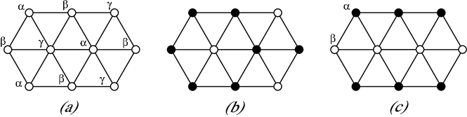
Figure 1: (a) The 3-sublattice decomposition of the triangular lattice; (b) Unperturbed configuration for $n=\frac{2}{3}$ (the filled circle represent occupied sites); (c) Unperturbed configuration for $n=\frac{1}{2}$.

The triangular lattice can be decomposed into three equivalent sublattices, which we denote $\alpha$, $\beta$, $\gamma$, as shown in Fig. 1(a). For filling $n=\frac{2}{3}$ the unperturbed ground state has two sublattices (say $\alpha$ and $\beta$) fully occupied and the third ($\gamma$) empty. This corresponds to a solid phase, with a density modulation with wavevector ${\bf k}=({4\pi\over 3},0)$, and is shown in Fig. 1(b). It is also referred to as the $\sqrt{3}\times\sqrt{3}$ phase. Although the ground state is threefold degenerate, these do not mix in any finite order of perturbation theory and we can start from one of the partners. Turning on the hopping term allows particles to occupy the other sublattice, and at some critical value $t_{c}$ the average sublattice occupancies will become equal. This represents the transition from solid to superfluid. An order parameter can be defined as

$$m\equiv\langle n_{\alpha}\rangle-\langle n_{\gamma}\rangle=3\langle n_{\alpha}\rangle-2$$ (6)

which equals 1(0) in the fully ordered (disordered) phase. The transition can also be located from the behaviour of nearest neighbour correlators $C_{\alpha\beta}\equiv\langle n_{\alpha}n_{\beta}\rangle$, or from the static structure factor

$$S({\bf k})={1\over N}\sum_{i,j}\langle n_{i}n_{j}\rangle e^{i{\bf k}\cdot({\bf R}_{j}-{\bf R}_{i})}$$ (7)

at ${\bf k}={\bf k}^{*}$, where ${\bf k}^{*}=({4\pi\over 3},0)$ is the wavevector for the $\sqrt{3}\times\sqrt{3}$ phase. For $n=\frac{1}{3}$ a completely analogous treatment can be used, with the unperturbed ground state having one sublattice (say $\gamma$) fully occupied, and the other sublattices empty.

At half-filling ($n=\frac{1}{2}$) the unperturbed system is equivalent to an isotropic Ising antiferromagnet in zero field, which is known to be disordered at $T=0$, with a macroscopic ground state degeneracy. It seems, however, that a nonzero hopping term lifts this degeneracy and leads to a stable supersolid phase - an example of the ‘order from disorder’ phenomenonsheng92 , induced by quantum fluctuations. To study this case via series expansions we include an additional field in the unperturbed Hamiltonian (and subtract it via the perturbation term), to choose a unique ground state. We choose the striped state shown in Fig. 1(c), for which a two-sublattice decomposition of the triangular lattice is made. This will be discussed further in Section IV.

III The $n=\frac{1}{3},\frac{2}{3}$ phases

We turn now to our results, considering first the commensurate phase with $n=\frac{2}{3}$. The unperturbed ground state ($\sqrt{3}\times\sqrt{3}$) is shown in Figure 1(b). The order parameter $m$ (Eqn. 6) will decrease with increasing $t$, and, assuming a normal 2nd order transition, will go to zero with a power law

$$m\sim(t_{c}-t)^{\beta},\quad t\to t_{c}^{-}$$ (8)

where $\beta$ is a critical exponent.

We have computed a series expansion for $m$, up to order $t^{12}$. The series coefficients are given in Table 1. Dlog Padé approximants (shown in Table 2) and integrated differential approximantsgut have been used to analyse this series, with the resulting estimates

$$t_{c}=0.21(1),\quad\beta=0.09(1)$$ (9)

The estimate $t_{c}=0.21$ is consistent with the most recent Monte Carlo estimatewes05 of $0.195\pm 0.025$. We are unaware of any previous estimate of the exponent $\beta$. The order and universality class of this transition remain unclear. Our exponent estimate $\sim 0.09(1)$ is similar to that of the 3-state Potts model in two dimensions ($\beta=1/9$). On the other hand the 3-state Potts model in three dimensions is believed to have a weak first-order transitions.

It would be straightforward to compute the order parameter for specific values of $t$, and to display a curve of $m(t)$, but we do not do this.

Figure 2: The ground state energy per site $E_{0}$ and $(d^{2}E_{0}/dt^{2})^{-1}$ versus $t$ for $n=2/3$ filling, the results of several different integrated differential approximants to the series are shown.

Figure 3: The nearest neighbor correlators $C_{\alpha\beta}$ and $C_{\alpha\gamma}$ and their difference, versus $t$, for $n=2/3$ filling. Several different integrated differential approximants to the series are shown.

An alternative way of estimating the critical point is to compute the series for the ground state energy $E_{0}(t)$ and for the second derivative $d^{2}E_{0}/dt^{2}$ (analogous to a ‘specific heat’). This analysis is less precise, but the results are consistent with (9). In Figure 2 we show $E_{0}$ and the inverse of the second derivative as functions of $t$, for $0<t\leq t_{c}$. The results of several different integrated differential approximants to the series are shown. The second derivative is seen to diverge at $t\sim 0.21$.

We have also obtained series in $t$ for the pair correlations $C_{ij}\equiv\langle n_{i}n_{j}\rangle$. One such series is given in Table 1) - we are happy to provide others on request. Figure 3 shows three curves, as functions of $t$: the nearest neighbor correlators $C_{\alpha\beta}$ and $C_{\alpha\gamma}$, and their difference. The difference $C_{\alpha\beta}-C_{\alpha\gamma}$ decreases from 1 as $t$ increases, and vanishes at the critical point where all sublattices are equally occupied. This gives an independent estimate of $t_{c}$, consistent with (9).

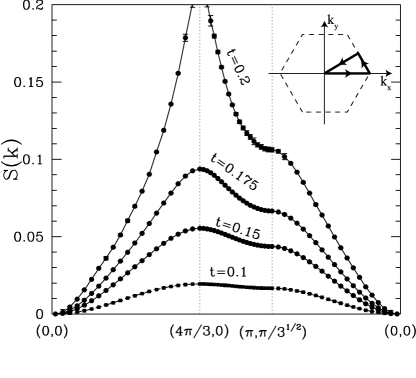
Figure 4: The static structure factor $S({\bf k})$ along high-symmetry cuts through the Brillouin zone for various $t$ at $n=2/3$ filling. The inset shows the Brillouin zone, and path chosen.

Figure 5: The static structure factor $S({\bf k}^{*})$ versus $t$ at $n=2/3$ filling. Several different integrated differential approximants to the series are shown. Since the series begins with a $t^{2}$ term we divide this out for convenience.

Another quantity of interest is the static structure factor

$$S({\bf k})={1\over N}\sum_{i,j}(\langle n_{i}n_{j}\rangle-\langle n_{i}\rangle\langle n_{j}\rangle)e^{i{\bf k}\cdot({\bf R}_{j}-{\bf R}_{i})}$$ (10)

This differs from the more usual definition (eq. Ref. bon03, ) by the subtraction of the second term, which is necessary to implement the linked cluster method efficiently. The effect of this term is to remove the $\delta$-function peak at ${\bf k}=0$, and reduce it at the special wavevector ${\bf k}^{*}$. At the transition point $t_{c}$, where $\langle n_{i}\rangle$ is independent of sublattice, the contribution of this second term vanishes, and our $S({\bf k})$ is expected to show a $\delta$-function peak at ${\bf k}^{*}$. This is confirmed in Figure 4, where we show $S({\bf k})$ curves along symmetry lines in the Brillouin zone for various $t$ values.

At ${\bf k}={\bf k}^{*}$, the Dlog Padé approximants to the series $S({\bf k}^{*})$ give a critical point estimate $t_{c}=0.208(3)$ with exponent $-0.40(3)$ (see Table 2). To obtain a more accurate estimate of $S({\bf k}^{*})$ versus $t$, we use integrated differential approximants to the series $[S({\bf k}^{*})]^{-2.5}$ (which vanishes linearly at $t_{c}$). The result is shown in Fig. 5, from which we can locate the critical point more accurately, at $t_{c}=0.208(1)$.

IV The $n=\frac{1}{2}$ Phase

As noted in Section II, the case of half-filling ($n=\frac{1}{2}$) is rather more subtle, as the unperturbed system has an infinitely degenerate ground state. To allow a series expansion we introduce an auxiliary field to break this degeneracy. There are many ways to do this, but the simples choice is to decompose the triangular lattice into two sublattices ($\alpha,\beta$) shown in Figure 1(c), and to impose a staggered field, which favours occupancy of the $\alpha$ sublattice. Thus the unperturbed Hamiltonian is

$$H_{0}=V\sum_{\langle ij\rangle}n_{i}n_{j}-h\sum_{i}\eta_{i}n_{i}$$ (11)

and the perturbation is

$$H_{1}=-t\sum_{\langle ij\rangle}(a_{i}^{\dagger}a_{j}+a_{j}^{\dagger}a_{i})+h\sum_{i}\eta_{i}n_{i}$$ (12)

where $\eta_{i}=+1,-1$ on sublattices $\alpha$, $\beta$ respectively. The full Hamiltonian is $H=H_{0}+\lambda V$. Perturbation series are derived in power of $\lambda$, and $\lambda=1$ corresponds to the original Hamiltonian. Note that the field terms cancel in this limit. The value of $h$ is arbitrary and can be chosen to obtain optimal convergence of the series.

Figure 6: The static structure factor $S({\bf k})$ along high-symmetry cuts through the Brillouin zone for $t=0.03,0.04,0.05$ at $n=1/2$ filling. The inset shows the Brillouin zone, and the path chosen.

We have derived series for the same quantities as in the previous Section: the ground state energy and the order parameter, $m\equiv\langle n_{\alpha}\rangle-\langle n_{\beta}\rangle$, to order $\lambda^{11}$, pair correlations and the structure factor to order $\lambda^{10}$. The series are evaluated as single variable series in $\lambda$, for fixed values of $t$, $h$. To estimate the critical value $t_{c}$ we proceed as follows. For any value of $t$ the series will have a singularity at $\lambda=\lambda_{c}(t)$ and $t_{c}$ is determined from the condition $\lambda_{c}(t_{c})=1$. For $t<t_{c}$, $\lambda_{c}$ is larger than 1, implying that the system retains the striped order shown in Figure 1(c) at $\lambda=1$, while for $t>t_{c}$, $\lambda_{c}$ is less than 1. The analysis is less precise than for the $n=\frac{1}{3}$, $\frac{2}{3}$ cases, but we obtain a consistent critical point at $t_{c}\simeq 0.06$. Table 3 presents a number of series, for the parameter choice $t=0.06$, $h=0.25$. Table 4 presents the results of a Dlog Padé approximant analysis. The order parameter series, in particular, is quite well behaved and shows a consistent sequence of estimates of $\lambda_{c}$ converging to $\lambda_{c}\simeq 1.0$. The series for correlators and for the structure factor give a similar conclusion, that $t_{c}\simeq 0.06$.

Figure 7: The static structure factor $S({\bf k}^{*})$ versus $t$ at $n=1/2$ filling.

In Figure 6 we show the structure factor along symmetry lines in the Brillouin zone for $n=\frac{1}{2}$. The ordering wavevector for the striped 2-sublattice ordered structure is ${\bf k}^{*}=2\pi(0,1/\sqrt{3})$ and we see the development of a divergent peak at ${\bf k}^{*}$, as $t\to 0.06$. There is also a peak at the ordering wavevector for the $\sqrt{3}\times\sqrt{3}$ phase. Figure 7 shows the divergence of $S({\bf k}^{*})$ as $t$ increases, towards 0.06.

Our estimate for the transition $t_{c}\sim 0.06$ is somewhat lower than the latest Monte Carlo estimatewes05 of $t_{c}\sim 0.115$. We discuss possible reasons for this in the final section of the paper.

V Conclusions

We have used series expansions to investigate the ground state phase diagram of the hard-core boson model on the triangular lattice, which is of considerable current interest. Series are derived in powers of the hopping parameter $t$, and hence probe the spatially ordered phases and transitions to a uniform superfluid phase. Series have been computed for the ground state energy, the order parameters, the near neighbour pair correlations and the static structure factor. All of these quantities show consistent results with each other.

At the commensurate densities $n=\frac{1}{3},\frac{2}{3}$ we locate a quantum phase transition at $(t/V)_{c}\simeq 0.208(1)$, in good agreement with the most recent Monte Carlo results of $0.195\pm 0.025$. The order parameter appears to vanish at $(t/V)_{c}$ with a power low, with an exponent $\beta\simeq 0.09$. At $n=\frac{1}{2}$ (half-filling) early Monte Carlo workbon03 indicated no ordered solid phase at any finite $t$, although the most recent workwes05 ; hei05 ; mel05 ; bon05 finds a supersolid phase persisting to $t/V\simeq 0.1$. To derive series expansion for this case we stabilize one of the infinite manifold of ground states (a ‘striped’ 2-sublattice phase) by applying an external field. This phase, which presumably is supersolid, appears stable to $t/V\sim 0.06$.

Using the present approach we are unable to probe off-diagonal long-range order and hence to study the superfluid phases.

We are also unable to exclude the possibility of weakly first-order rather than second-order transitions. In this context we mention recent field theoretical workbur05 , which argues that the transitions in this model lie in the class of ‘deconfined quantum critical points’.

Table 1: Series for ground state energy per site $E_{0}(t)$, order parameter $m$, difference of shortest correlator $C_{\alpha\beta}-C_{\alpha\gamma}$, and static structure factor $S$ at ${\bf k}^{*}$ for the $n=2/3$ case. Nonzero coefficients $t^{n}$ up to order $n=12$ are listed.

$n$	$E_{0}(t)$	$m$	$C_{\alpha\beta}-C_{\alpha\gamma}$	$S({\bf k}^{*})$
0	1.000000000	1.000000000	1.000000000	0.000000000
1	0.000000000	0.000000000	0.000000000	0.000000000
2	$-$1.000000000	$-$2.250000000	$-$2.750000000	1.500000000
3	$-$1.000000000	$-$4.500000000	$-$5.500000000	3.000000000
4	$-$9.500000000$\times 10^{-1}$	$-$1.019750000$\times 10^{1}$	$-$1.052083333$\times 10^{1}$	8.168333333
5	$-$2.355555556	$-$3.750666667$\times 10^{1}$	$-$3.819305556$\times 10^{1}$	3.518166667$\times 10^{1}$
6	$-$7.937379630	$-$1.418886375$\times 10^{2}$	$-$1.498124375$\times 10^{2}$	1.428442162$\times 10^{2}$
7	$-$2.616389136$\times 10^{1}$	$-$5.619014174$\times 10^{2}$	$-$5.933175977$\times 10^{2}$	6.107654281$\times 10^{2}$
8	$-$9.005836612$\times 10^{1}$	$-$2.307990196$\times 10^{3}$	$-$2.428296319$\times 10^{3}$	2.667494106$\times 10^{3}$
9	$-$3.229654053$\times 10^{2}$	$-$9.596323715$\times 10^{3}$	$-$1.008214369$\times 10^{4}$	1.170747249$\times 10^{4}$
10	$-$1.201486606$\times 10^{3}$	$-$4.067064188$\times 10^{4}$	$-$4.264450526$\times 10^{4}$	5.234712003$\times 10^{4}$
11	$-$4.607510926$\times 10^{3}$	$-$1.750821492$\times 10^{5}$	$-$1.832564264$\times 10^{5}$
12	$-$1.792870548$\times 10^{4}$	$-$7.572580451$\times 10^{5}$

Table 2: $[n/m]$ Dlog Padé approximants to the series of $d^{2}E_{0}/dt^{2}$, $m$, $C_{\alpha\beta}-C_{\alpha\gamma}$, and $S({\bf k}^{*})$ for $n=2/3$ case. The position of the singularity (pole), the critical index (index) from unbiased approximants are given. An asterisk denotes a defective approximant.

n	$[(n-2)/n]$	$[(n-1)/n]$	$[n/n]$	$[(n+1)/n]$	$[(n+2)/n]$
	pole (index)	pole (index)	pole (index)	pole (index)	pole (index)
$d^{2}E_{0}(t)/dt^{2}$
n=1		1.2500($-$3.750)	0.0518($-$0.006)	0.1834($-$0.286)	0.1929($-$0.350)
n=2	0.2342($-$0.388)	0.1514($-$0.139)	0.1936($-$0.357)	0.1953($-$0.373)	0.1921($-$0.345)*
n=3	0.1726($-$0.213)	0.1951($-$0.371)	0.1933($-$0.355)*	0.2124($-$0.845)	0.2007($-$0.438)
n=4	0.2111($-$0.691)	0.2020($-$0.463)	0.2010($-$0.444)	0.2036($-$0.502)
n=5	0.2006($-$0.438)	0.2018($-$0.459)
$m$
n=1			0.3333(0.5000)	0.2651(0.2517)	0.2138(0.1064)
n=2		0.2750(0.2896)	0.1673(0.0261)	0.2209(0.1246)	0.2180(0.1162)
n=3	0.2368(0.1741)	0.2257(0.1411)	0.2164(0.1109)	0.1999(0.0504)	0.2126(0.0986)
n=4	0.1852(0.0262)	0.2103(0.0897)	0.2116(0.0946)	0.2108(0.0910)	0.2087(0.0809)
n=5	0.2121(0.0965)	0.2111(0.0925)	0.2168(0.0994)*	0.2100(0.0876)
n=6	0.2096(0.0860)	0.2104(0.0895)
$C_{\alpha\beta}-C_{\alpha\gamma}$
n=1			0.3333(0.6111)	0.2884(0.3959)	0.2146(0.1213)
n=2		0.2932(0.4219)	0.1049(0.0019)	0.2207(0.1393)	0.2182(0.1309)
n=3	0.2431(0.2229)	0.2288(0.1712)	0.2166(0.1247)	0.1983(0.0487)	0.2134(0.1134)
n=4	0.1906(0.0404)	0.2115(0.1047)	0.2123(0.1079)	0.2111(0.1025)	0.2090(0.0905)
n=5	0.2124(0.1087)	0.2118(0.1058)	0.1988(0.0307)*
n=6	0.2100(0.0970)
$S({\bf k}^{*})$
n=1		0.2902($-$0.5805)	0.1508($-$0.1568)	0.2228($-$0.5051)	0.2001($-$0.3291)
n=2	0.1833($-$0.2678)	0.1941($-$0.3066)	0.2052($-$0.3709)	0.2051($-$0.3700)	0.2152($-$0.5228)
n=3	*	0.2051($-$0.3700)	0.2052($-$0.3709)	0.2072($-$0.3895)
n=4	0.2082($-$0.4033)	0.2081($-$0.4024)

Table 3: Series for ground state energy per site $E_{0}$, order parameter $m$, difference of shortest correlator $C_{\alpha\alpha}-C_{\alpha\beta}$ and $C_{\alpha\alpha}-C_{\beta\beta}$, and static structure factor $S$ at ${\bf k}^{*}=(0,2\pi/\sqrt{3})$ for $t=0.06$ and the field $h=0.25$ at $n=1/2$ case. Nonzero coefficients $\lambda^{n}$ up to order $n=11$ are listed.

$n$	$E_{0}$	$m$	$C_{\alpha\alpha}-C_{\alpha\beta}$	$C_{\alpha\alpha}-C_{\beta\beta}$	$S({\bf k}^{*})$
0	5.000000000$\times 10^{-1}$	1.000000000	1.000000000	1.000000000	0.000000000
1	0.000000000	0.000000000	0.000000000	0.000000000	0.000000000
2	$-$4.800000000$\times 10^{-3}$	$-$1.280000000$\times 10^{-2}$	$-$1.760000000$\times 10^{-2}$	$-$1.280000000$\times 10^{-2}$	1.280000000$\times 10^{-2}$
3	$-$1.984000000$\times 10^{-3}$	$-$1.058133333$\times 10^{-2}$	$-$1.454933333$\times 10^{-2}$	$-$1.058133333$\times 10^{-2}$	1.058133333$\times 10^{-2}$
4	$-$8.346453333$\times 10^{-4}$	$-$6.818781867$\times 10^{-3}$	$-$9.282071467$\times 10^{-3}$	$-$6.818781867$\times 10^{-3}$	6.969821867$\times 10^{-3}$
5	$-$3.763032178$\times 10^{-4}$	$-$4.322561214$\times 10^{-3}$	$-$5.768006277$\times 10^{-3}$	$-$4.322561214$\times 10^{-3}$	4.758822760$\times 10^{-3}$
6	$-$1.920603977$\times 10^{-4}$	$-$2.973745768$\times 10^{-3}$	$-$3.879098112$\times 10^{-3}$	$-$2.973745768$\times 10^{-3}$	3.673001969$\times 10^{-3}$
7	$-$1.129137214$\times 10^{-4}$	$-$2.252261754$\times 10^{-3}$	$-$2.888143560$\times 10^{-3}$	$-$2.252261754$\times 10^{-3}$	3.111869445$\times 10^{-3}$
8	$-$7.425851217$\times 10^{-5}$	$-$1.819385962$\times 10^{-3}$	$-$2.309557263$\times 10^{-3}$	$-$1.819385962$\times 10^{-3}$	2.744159087$\times 10^{-3}$
9	$-$5.242495609$\times 10^{-5}$	$-$1.520557155$\times 10^{-3}$	$-$1.918242621$\times 10^{-3}$	$-$1.520557155$\times 10^{-3}$	2.454367694$\times 10^{-3}$
10	$-$3.867629129$\times 10^{-5}$	$-$1.296181354$\times 10^{-3}$	$-$1.627204515$\times 10^{-3}$	$-$1.296181354$\times 10^{-3}$	2.215862063$\times 10^{-3}$
11	$-$2.946020021$\times 10^{-5}$	$-$1.122501973$\times 10^{-3}$

Table 4: $[n/m]$ Dlog Padé approximants to the series of $d^{2}E_{0}/d\lambda^{2}$, $m$, $C_{\alpha\alpha}-C_{\alpha\beta}$, $C_{\alpha\alpha}-C_{\beta\beta}$, and $S({\bf k}^{*})$ for $t=0.06$ and the field $h=0.25$ at $n=1/2$ case. The position of the singularity (pole), the critical index (index) from unbiased approximants are given. An asterisk denotes a defective approximant.

n	$[(n-2)/n]$	$[(n-1)/n]$	$[n/n]$	$[(n+1)/n]$	$[(n+2)/n]$
	pole (index)	pole (index)	pole (index)	pole (index)	pole (index)
$d^{2}E_{0}/d\lambda^{2}$
n=1		2.2586($-$2.8007)	1.4547($-$1.1617)	0.9731($-$0.3478)	0.9220($-$0.2803)
n=2	1.6180($-$1.5630)	0.7556($-$0.1148)	0.9164($-$0.2716)	0.9458($-$0.3145)	1.1581($-$6.1720)*
n=3	0.9303($-$0.2941)	1.0207($-$0.4982)	1.0060($-$0.4512)	0.9990($-$0.4284)	0.9929($-$0.4076)
n=4	1.0063($-$0.4522)	0.9889($-$0.3895)	0.9707($-$0.3098)
n=5	0.9711($-$0.3113)
$m$
n=1		*	0.8065(0.0166)	1.1500(0.0483)	1.2383(0.0649)
n=2	*	1.3497($-$0.0279)*	1.2735(0.0755)	1.2075(0.0577)	1.3029(0.0748)*
n=3	1.1914(0.0521)	1.1288(0.0392)	1.0916(0.0316)	1.0711(0.0271)	1.0576(0.0241)
n=4	1.0746(0.0277)	1.0591(0.0243)	1.0364(0.0187)	1.0094(0.0124)	0.9977(0.0100)
n=5	0.9887(0.0083)	0.9929(0.0090)	0.9946(0.0094)
n=6	0.9962(0.0097)
$C_{\alpha\alpha}-C_{\alpha\beta}$
n=1		*	0.8065(0.0229)	1.1563(0.0675)	1.2532(0.0931)
n=2	*	1.3327($-$0.0378)*	1.2969(0.1123)	1.2229(0.0830)	1.3011(0.1043)*
n=3	1.2075(0.0751)	1.1419(0.0559)	1.1015(0.0443)	1.0783(0.0373)	1.0631(0.0326)
n=4	1.0820(0.0382)	1.0643(0.0327)	1.0407(0.0251)	1.0149(0.0171)
n=5	1.0014(0.0133)	0.9989(0.0127)
$C_{\alpha\alpha}-C_{\beta\beta}$
n=1		*	0.8065(0.0166)	1.1500(0.0483)	1.2383(0.0649)
n=2	*	1.3497($-$0.0279)*	1.2735(0.0755)	1.2075(0.0577)	1.3029(0.0749)*
n=3	1.1914(0.0521)	1.1288(0.0392)	1.0916(0.0316)	1.0711(0.0271)	1.0576(0.0241)
n=4	1.0746(0.0277)	1.0591(0.0242)	1.0364(0.0187)	1.0094(0.0124)
n=5	0.9887(0.0083)	0.9929(0.0090)
$S({\bf k}^{*})$
n=1		2.0378($-$1.6846)	1.2297($-$0.6135)	0.9509($-$0.2837)	0.9605($-$0.2952)
n=2	1.4031($-$0.8844)	0.8620($-$0.1860)	0.9602($-$0.2948)	0.9482($-$0.2815)*	1.0447($-$0.4819)
n=3	0.9726($-$0.3144)	1.0375($-$0.4476)	1.0246($-$0.4121)	1.0163($-$0.3890)
n=4	1.0250($-$0.4132)	0.9918($-$0.3047)