Diffusive Atomistic Dynamics of Edge Dislocations in Two Dimensions

Abstract

The fundamental dislocation processes of glide, climb, and annihilation are studied on diffusive time scales within the framework of a continuum field theory, the Phase Field Crystals (PFC) model. Glide and climb are examined for single edge dislocations subjected to shear and compressive strain, respectively, in a two dimensional hexagonal lattice. It is shown that the natural features of these processes are reproduced without any explicit consideration of elasticity theory or ad hoc construction of microscopic Peierls potentials. Particular attention is paid to the Peierls barrier for dislocation glide/climb and the ensuing dynamic behavior as functions of strain rate, temperature, and dislocation density. It is shown that the dynamics are accurately described by simple viscous motion equations for an overdamped point mass, where the dislocation mobility is the only adjustable parameter. The critical distance for the annihilation of two edge dislocations as a function of separation angle is also presented.

I Introduction

Plastic flow in periodic systems is typically mediated by the motion of line defects or dislocations. The largest challenge in developing a meaningful theory of plasticity is often linking the microscopic behavior of individual, discrete dislocations to the macroscopic plastic behavior of the system. In atomic and molecular crystals for example, understanding the effect of dislocations on mesoscopic and macroscopic material properties involves the treatment of length and time scales that capture the relevant dynamics of individual dislocations ($\sim$$10^{-12}s$,$\sim$$10^{-9}m$) through those that describe the macroscopic response of the material ($\sim$$10^{1}s$,$\sim$$10^{-2}m$). An important approach to the problem of spanning this large range of scales has been to measure the dynamics of individual dislocations and/or small numbers of interacting dislocations on the shortest time scales from Molecular Dynamics (MD) simulations chang99 ; chang02 ; bailey01 ; rodary04 . These results are then used as input into coarse-grained, mesoscopic simulations such as Dislocation Dynamics (DD) dd90 ; bulatov98 , which can provide information on systems with large numbers of dislocations under the action of experimentally accessible strains and strain rates.

In this study, dislocation dynamics are examined on length scales comparable to those encountered in MD simulations, but over diffusive time scales and using experimentally accessible strain rates. This approach provides a single framework that removes the vibrational time scales, while all of the relevant length scales can potentially be reached with greater computing power or with more advanced numerical techniques nigel05 . In addition to atomic crystals, the results presented here may be interpreted in terms of other periodic systems such as Abrikosov vortex lattices in superconductors pardo98 , magnetic thin films sagui95 ; orlikowski99 , block copolymers harrison00 , oil-water systems containing surfactants laradji91 , and colloidal crystals.

The PFC model describes periodic systems of a continuum field nature and naturally incorporates elastic and plastic behavior. The details of the model have been presented elsewhere ken01 , and only the necessary equations will be given here. The dimensionless free energy functional is written as

$$F=\int{d\vec{x}\bigg{[}{\rho\over 2}\omega(\nabla^{2})\rho+{\rho^{4}\over 4}\bigg{]}}$$ (1)

where $\rho$ is an order parameter corresponding here to density and

$$\omega(\nabla^{2})=r+(1+\nabla^{2})^{2}.$$ (2)

$r$ is a phenomenological constant related to temperature. The dynamics of $\rho$ are described by

$${\partial{\rho}\over\partial{t}}=\nabla^{2}\frac{\delta F}{\delta\rho}+\zeta=\nabla^{2}(\omega(\nabla^{2})\rho+\rho^{3})+\zeta$$ (3)

where $\zeta$ is a gaussian random noise variable ($\langle\zeta(\vec{r}_{1},t_{1})\zeta(\vec{r}_{2},t_{2})\rangle=D\nabla^{2}\delta(\vec{r}_{1}-\vec{r}_{2})\delta(\tau_{1}-\tau_{2})$ and $D=uk_{B}Tq_{0}^{d-4}/\lambda^{2}$) which has been largely neglected in this study, as will be discussed in Section III.

In Section II, the details of how the PFC model is adapted to numerical simulation are outlined, and in Section III the simulation results for glide, climb, and annihilation are presented and analyzed. Section IV includes a summary, comparison with other recent phase field simulations of dislocations, and discussion of further developments.

II Simulation Method

II.1 Discretization, Initial Conditions, and Boundary Conditions

Eq. (3) was solved numerically in two dimensions using the ’spherical laplacian’ approximation for $\nabla^{2}$ oono_puri and a forward Euler discretization for the time derivative. Periodic boundary conditions were applied in all directions for glide simulations and mirror boundary conditions were used perpendicular to the climb direction in climb simulations. To create a system with a single edge dislocation, an initial condition consisting of a hexagonal one-mode solution for $\rho(x,y)$ was applied with N atoms/row in the lower half and N+1 atoms/row in the upper half. The hexagonal state is expressed analytically as

$$\rho(x,y)=A\bigg{[}\cos{(qx)}\cos{({qy\over\sqrt{3}})}-{1\over 2}\cos{({2qy\over\sqrt{3}})}\bigg{]}+\rho_{0}$$ (4)

where

$$A={4\over 5}\bigg{(}\rho_{0}+{1\over 3}\sqrt{-15r-36\rho_{0}^{2}}\bigg{)},$$ (5)

$q$ is the numerically determined equilibrium wavenumber for a hexagonal state at a given value of $r$, and $\rho_{0}$ is the average density. In glide simulations, the hexagonal state was bounded at its upper and lower edges by a constant, or liquid, state of width approximately $4a_{y}$, where $a_{y}$ is the equilibrium lattice parameter in the $y$-direction (Fig. 1). The same approach was used in the climb simulations, except that the liquid was placed along the sides. Before applying strain, all systems were allowed to equilibrate until their free energy no longer changed with time.

At a given value of $r$, the value of $\rho_{0}$ for the hexagonal portion of the simulation was set to fall on the phase boundary between the hexagonal and hexagonal/constant coexistence regions. The value of $\rho_{0}$ for the liquid portion of the simulation was set to fall on the boundary between the hexagonal/constant coexistence region and the constant phase region. This was necessary to make the interfaces between the hexagonal and constant phases stable, with no preference toward crystallization or melting. A drawback is that this makes any comparison of results at different $r$ values indirect, since $\rho_{0}$ must vary with $r$. For this reason the boundary conditions were changed when the $r$ dependence of the dynamics was of interest. Details are discussed in the following section.

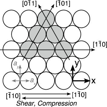
Figure 1: Schematic of (111) plane in a FCC crystal corresponding to the 2D system of interest.

II.2 Strain Application

Two methods were used to apply strain to the system. In both, $\rho(x,y)$ was coupled to an external field along the outer two rows of particles bounding the liquid phase on each side of the system. This external field was set to the one-mode solution given in Eq. (4), and for glide (climb) was moved in the positive $x$-direction along the lower (left) rows and in the negative $x$-direction along the upper (right) rows, both at the same constant velocity. The particles in the system are energetically motivated to follow the motion of these fields, giving the effect of a physically applied strain.

In the first method, which will be called rigid displacement, Eq. (3) was solved in the presence of the external fields, but in addition, the particles between the external fields were rigidly displaced along with the motion of the fields to ensure a linear strain profile across the width of the system. In the second method, this rigid displacement was not enforced, allowing the strain profile to take whichever form the dynamics of Eq. (3) dictate. This method will be called relaxational displacement. In Section III, it will be shown that the dynamic behavior of the dislocations can be significantly influenced by which method is used and that the two methods may be viewed as limiting cases of rigid and diffusive response. From this viewpoint, rigid displacement describes atomic crystals and relaxational displacement applies to ’softer’ systems such as colloidal crystals, superconducting vortex lattices, magnetic films, oil-water systems containing surfactants, and block copolymers.

II.3 Symmetries and Time Scales

The crystalline symmetry here is equivalent to the {111} family of planes in a FCC lattice or the {0001} family of planes in a HCP lattice, for example. These close packed planes and the subsequent glide directions compose the primary slip systems in many common types of ductile, metallic crystals. Using the FCC lattice as a reference, application of shear in this geometry results in glide along a $\langle 110\rangle$ direction within a {111} slip plane, as shown in Fig. 1. The directions in a HCP lattice would fall in the $\langle 11\bar{2}0\rangle$ family. Climb in this geometry was made to occur along a $\langle\bar{1}\bar{1}2\rangle$ direction. Shear and compression were also applied over various other rotations as will be discussed briefly in the following.

System sizes ranging from 676 to 56,952 particles were examined, and strain rates ranging from 2$\times 10^{-7}/t$ to 1$\times 10^{-2}/t$ were used, where $t$ is the dimensionless time introduced in Eq. (3). These strain rates can be expressed in physical units by matching the time scales of the model to those of typical metals near their respective melting temperatures. This is done by equating vacancy diffusion constants, $D_{v}$, which have been calculated analytically for this model in ken04 , and which may range from $10^{-8}$–$10^{-13}cm^{2}/s$ for typical metals lubensky85 . Lattice constants, $a$, must also be equated to return to physical units. Using Cu at $1063^{\circ}\mathrm{C}$ as a reference ($D_{v}\simeq 10^{-9}cm^{2}/s$, $a\simeq 3.61$Å), and matching to the model at $r=-0.8$ ($D_{v}=1.78a^{2}/t$), the range of strain rates used converts to .09/$s$–4500/$s$. Using these same parameters, the dislocation velocities observed are on the order of $10^{-7}$–$10^{-4}m/s$, a range well below the acoustic limit and accessible by experiment. The dislocation densities range from approximately $10^{10}$–$10^{12}/cm^{2}$.

II.4 Simulation Output: A Preliminary Example

Before presenting the analysis of all simulation data, the output from a single glide simulation will be presented to clarify various definitions and results that will be of importance in interpreting the data. The collective results from all simulations will be analyzed further in the following section.

Four primary types of output were generated in each simulation, from which all properties of interest were extracted. The variables are the instantaneous position and velocity of the dislocation, and the strain and change in free energy of the system, all recorded as functions of time as shown in Fig. 2. The gray lines represent theoretical results which will be presented in Section III.

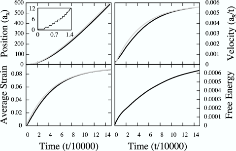
Figure 2: One set of simulation data (black lines) and the corresponding theoretical results (gray lines) for glide. Parameters are $r=-0.4$, ($L_{x},L_{y}$)=(60,56), and $\dot{\gamma}=2\times 10^{-6}/t$ The inset in the upper left corner of the upper left plot shows a magnification of the position vs. time data at early times to emphasize the stick-slip nature of the motion at low velocities.

The position was determined by locating all maxima of $\rho(x,y)$ (which can be considered the discrete particle locations) and counting the number of nearest neighbors for each. Any maxima with more or less than six nearest neighbors must be near the dislocation core, and by averaging the positions of all maxima identified in this way, an overall dislocation position was inferred. The velocity was then calculated from the slope of the position versus time data.

The average shear strain in the system, $\bar{\gamma}$, was measured by again locating the peaks in $\rho(x,y)$, and noting that in equilibrium, each particle will have another particle located a distance of $2a_{y}$ away in the positive $y$-direction. If this particle is found to be offset some distance, $dx_{i}$, in the $x$-direction, then the local shear strain is equal to $dx_{i}/2a_{y}$. The average shear strain in the system is then given by

$$\bar{\gamma}=\frac{1}{2Na_{y}}\sum_{i=1}^{N}dx_{i}$$ (6)

where $N$ is the number of particles in the system. The fourth variable, the average free energy $F$, was simply calculated from Eq. (1) at regular intervals of time.

The Peierls barrier is a measure of the resistance to the onset of motion in a periodic system. In these simulations, the barrier is defined as the amount of strain that has been applied at the instant that the dislocation has precessed a distance of one lattice constant. $\gamma_{P}$ and $\epsilon_{P}$ will denote the Peierls barriers for glide and climb, respectively. For clarity, Fig. 3 shows $\bar{\gamma}$ as a function of time for a few different values of $\dot{\gamma}$. The strain corresponding to this definition of $\gamma_{P}$ is indicated on each curve and can be seen to correspond to the point where the measured strain begins to deviate from the applied strain. The deviation is due to the strain relieved by the motion of the dislocation, as will be discussed in the next section.

Figure 3: Corrected and uncorrected $\bar{\gamma}$ versus time at $r=-0.4$ and $(L_{x},L_{y})=(60,56)$ for various values of $\dot{\gamma}$. The strain at which $\gamma_{P}$ is defined has been highlighted on each curve.

III Results and Analysis

III.1 Equilibrium Dislocation Geometry

Following equilibration as described in the previous section, the dislocations were found to reach one of the two stable configurations shown in Fig. 4. Which of the two configurations is selected depends sensitively on the details of the boundary conditions as well as on the system size. Systems larger in the $x$-direction tend to favor Config. 1, and systems larger in the $y$-direction tend to favor Config. 2, apparently due to the greater strain relief available at larger extensions. Systems with approximately equivalent $x$ and $y$ dimensions that were equilibrated with thermal noise oscillated between Configs. 1 and 2, indicating that the two states are approximately equivalent energetically. It will be shown in the following section that the initial configuration affects $\gamma_{P}$ but not the velocity of the dislocation.

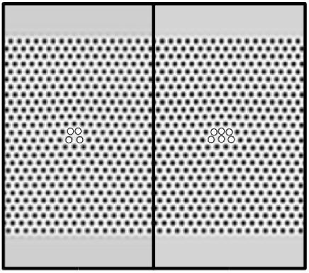
Figure 4: Stable dislocation configurations: The greyscale represents $\rho(x,y)$ and the particles around the dislocation core have been highlighted for clarity. Left: Config. 1. Right: Config. 2.

The average shear strain, $\bar{\gamma}$, in each system was measured and the values recorded following equilibration have been plotted in Fig. 5 as a function of $1/L_{y}$, where $L_{y}$ is the number of particles in the $y$-direction. A simple analysis reveals that the total $\bar{\gamma}$ due to an edge dislocation in this geometry is equal to $\sqrt{3}b/(4L_{y})$, where $b$ is the burger’s vector of the dislocation. This result agrees well with the measured values shown in Fig. 5, indicating that the measurement technique is reliable.

Figure 5: Equilibrium elastic strain, $\bar{\gamma}$, due to an edge dislocation plotted as a function of inverse system size in the $y$-direction. $L_{x}$ was fixed at 56 particles for the data shown.

III.2 Glide: Constant Applied Shear Rate Dynamics

Simulations were conducted using steady shear over a range of applied shear rates ($\dot{\gamma}$), temperatures ($r$), and system sizes ($L_{x},L_{y}$). The dependence of the Peierls barrier and the velocity vs. $\bar{\gamma}$ behavior on these variables will be discussed in the following subsections.

III.2.1 Peierls Barrier for Glide

To test for finite size effects, $\gamma_{P}$ was measured as a function of system size, or inverse dislocation density. Within estimated errors, no change was observed under rigid displacement as the system size was increased from 676 to 56,952 particles. Under relaxational displacement, a slight increase with $L_{y}$ was noted, and is linked to the time required for the strain applied at the edges to diffuse inward to the dislocation core. Diffusion is fast compared to the inverse shear rates required to apply relaxational displacement (rows of particles slip relative to each other at all but the lowest values of $\dot{\gamma}$), so the increase of $\gamma_{P}$ with $L_{y}$ cannot be very large. The nonlinear shear profile that is produced may exaggerate this lag between the applied strain and the strain near the dislocation, but the overall effect was nonetheless found to be relatively small.

Next, the barrier was examined as a function of $r$, which is proportional to the distance in temperature from $T_{c}$. To do this consistently, the boundary conditions were changed to mirror rather than periodic at the top and bottom, and the constant phase was entirely removed from the simulation. This made it possible to vary $r$ at a single value of $\rho_{0}$, isolating the temperature dependence in a more realistic manner. Results are shown in Fig. 6.

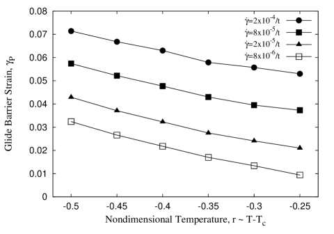
Figure 6: Temperature dependence of the Peierls strain barrier for glide without thermal fluctuations. Data shown is at $\rho_{0}=0.25$ and ($L_{x},L_{y}$)=(56,56) under rigid displacement.

The decrease in $\gamma_{P}$ as the melting point is approached is expected since the hexagonal phase becomes less pronounced near $T_{c}$. That is, $A$ decreases with increasing $r$ according to Eq. (5), and even without thermal fluctuations a distinct temperature dependence is produced. This decrease in $A$ corresponds to an increase in the width of the dislocation which, according to the Peierls-Nabarro model phillips , lowers the Peierls barrier for glide. With thermal fluctuations, these results did not change significantly, though at low $\dot{\gamma}$, which is where the change would be greatest, it was not possible to include fluctuations and maintain reasonable computation times. Similar linear decreases in $\gamma_{P}$ as some effective $T_{c}$ is approached have been found in experiment wasserbach86 ; lachenmann70 and theory cuitino01 ; tang99 , along with increases in $\gamma_{P}$ with $\dot{\gamma}$ much like those shown in Fig. 6.

At temperatures closer to the melting point ($r\simeq-0.18$), the dislocations began to climb at very low strains before any glide had occurred. This is the first evidence that climb is the dominant process at high temperatures, as in real crystals. Further evidence will be presented with the climb results.

The dependence of $\gamma_{P}$ on $\dot{\gamma}$ was also explicitly measured (Fig. 7). Both methods of shear application result in what appears to be a power law increase in $\gamma_{P}$ as the shear rate is increased, where the relaxational displacement data is nearly linear and the rigid displacement data appears to approach a limit $\gamma_{P}$ at high $\dot{\gamma}$.

Figure 7: Measured Peierls strain barrier for glide, $\gamma_{P}$, as a function of applied strain rate for the cases of rigid and relaxational displacement. The fits to the relaxational data are from Eq. (9) and the fits to the rigid data are power laws as indicated in the image. The dotted line shows a linear $\dot{\gamma}$ dependence for reference. Note that $\gamma_{P}$ is consistently lower for Config. 2 than for Config. 1, even with the differing $r$’s working toward the opposite effect.

This increase is explained as follows. Extrapolating the data to $\dot{\gamma}=0$ indicates that in all cases there is some small strain $\gamma_{P}^{0}<0.5\%$ at which the dislocation will glide, given sufficient time. Call this time from when $\gamma_{P}^{0}$ is reached to when the first glide event actually occurs $\Delta t_{hop}$. In any given simulation, once $\bar{\gamma}>\gamma_{P}^{0}$, excess strain is being applied during the interval $\Delta t_{hop}$ which makes the observed $\gamma_{P}$ appear to be larger than $\gamma_{P}^{0}$. In this approximation

$$\gamma_{P}=\gamma_{P}^{0}(r)+\dot{\gamma}\Delta t_{hop}(r)$$ (7)

which predicts a linear increase in $\gamma_{P}$ above $\gamma_{P}^{0}$. It is reasonable to expect though, that $\Delta t_{hop}$ will decrease at higher strain rates due to the additional strain applied during the interval. In a first approximation then

$$\Delta t_{hop}(r,\dot{\gamma})=\Delta t_{hop}^{0}(r)-\alpha(r)\eta(d,\dot{\gamma})\dot{\gamma}$$ (8)

where $\Delta t_{hop}^{0}(r)$ is the time required to execute a glide event at $\dot{\gamma}=0$ and $\alpha(r)$ is a coefficient related to the magnitude of the additional driving force applied during $\Delta t_{hop}$. $\eta(d,\dot{\gamma})$ is a coefficient related to the efficiency of strain transfer from the sample edges where strain is applied to the dislocation core, as a function of the type of displacement $d$ and $\dot{\gamma}$. $\eta(d,\dot{\gamma})=1$ for rigid displacement and drops below $1$ under relaxational displacement.

Substituting Eq. (8) into Eq. (7) gives

$$\gamma_{P}=\gamma_{P}^{0}(r)+\dot{\gamma}\Delta t_{hop}^{0}(r)-\alpha(r)\eta(d,\dot{\gamma})\dot{\gamma}^{2}$$ (9)

which now indicates a dependence on $\dot{\gamma}$ that must be fall below the initial expected linear trend. And the deviation from linear will be greatest under rigid displacement, since $\eta$ is maximum in this case. The data is in agreement with this expectation. Using $\gamma_{P}^{0}(-0.4)=\gamma_{P}^{0}(-0.8)=0.0038$, $\Delta t_{hop}(-0.4)=7277t$, $\Delta t_{hop}(-0.8)=6643t$, and $\alpha(-0.4)\eta=\alpha(-0.8)\eta=1.48\times 10^{-8}t^{2}$ produces reasonable fits to the relaxational displacement data shown in Fig. 7. Note that if $\Delta t_{hop}$ is negligible, then clearly this effect will not be noticeable, but since the dynamics are necessicarily diffusive in these simulations, it is reasonable to expect some contribution from this effect.

Accurate fits to the rigid displacement data were more difficult to obtain, most likely due to the transition to no $\dot{\gamma}$ dependence for large $\dot{\gamma}$. This can be shown by studying the evolution of $F$ under an applied shear. In ken04 , the change in $F$ for a one-mode approximate hexagonal solution under the action of shear was be found by minimizing $F$ when $\rho(x,y)$ is replaced with $\rho(x+\bar{\gamma}y,y)$. The resulting equation, valid for small $\bar{\gamma}$, is

$$\Delta F_{Shear}=\frac{q^{4}_{eq}A^{2}}{6}\bar{\gamma}^{2}.$$ (10)

In principle, this represents a rigid displacement of $\rho(x,y)$ at infinitely large $\dot{\gamma}$. In this limit, $\gamma_{P}$ has no explicit dependence on $\dot{\gamma}$;

$$\gamma_{P}=\sqrt{\frac{6\Delta F_{P}^{Glide}(\rho_{0},r)}{q^{4}_{eq}A^{2}}}.$$ (11)

Dislocation dynamics in soft structures such as colloidal crystals are reasonably expected to correspond to the case of relaxational displacement. These systems typically exhibit very little rigidity associated with sound modes or phonons, thus their relative softness. Conversely, dynamics in atomic crystals are believed to correspond to the case of rigid displacement at large $\dot{\gamma}$. Atomic crystals exhibit a significant rigidity in response to an applied shear, which can be reasonably approximated by a linear shear profile as is done for rigid displacement. A more constructive way to model atomic crystals would be to explicitly consider a phonon or wave term in the dynamics, as is being done by other authors mpfc . If such modes were considered, the collective motion of particles in response to an applied force would naturally be enhanced, more resembling the case of rigid displacement. It is argued in this sense that the methods of rigid displacement in the large $\dot{\gamma}$ region and relaxational displacement represent limiting cases of response, and that a more rigorous description including effective phonon dynamics would fall between these limits.

III.2.2 Atomistic Glide Mechanism

The nature of the dislocation motion in these simulations (Fig. 8) is stick-slip at low velocities with a transition to a more continuous character at high velocities. This is expected, as the lattice barrier leads to thermally activated motion when $\Delta F_{Shear}$ approximately equals $\Delta F_{P}^{Glide}$, while at large values of $\Delta F_{Shear}$ the barrier becomes secondary and the motion assumes a damped character. The shear rate dictates the maximum velocity and therefore the extent to which the motion becomes continuous. Three regimes of motion were observed, with selection depending on the ratio

$$v_{ss}=\frac{\dot{\gamma}}{\rho_{d}b}$$ (12)

where $\rho_{d}$ is the dislocation density dictated by the system size. The reason for labeling this quantity $v_{ss}$ will soon become apparent.

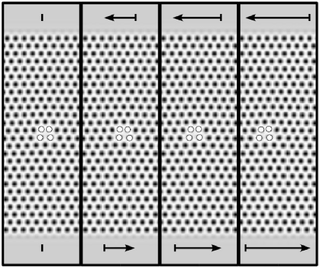
Figure 8: Atomistic glide mechanism under constant applied shear rate (the particles around the dislocation core have been highlighted for clarity). From left to right, $\rho(x,y)$ is shown at $t$=0, 500, 1000, and 1500, corresponding to $\bar{\gamma}$=1$\%$, 2$\%$, 3$\%$, and 4$\%$. The arrows indicate relative strain magnitudes and directions.

For large $v_{ss}$ ($\gtrsim 0.016a/t$), the dislocation quickly reaches the overdamped regime and adjacent layers of particles begin to slip relative to each other along the $x$-direction before a steady-state velocity is achieved. Slipping usually occurs when the strain exceeds approximately 20% in rigid displacement or 10–15% in relaxational displacement. At moderate values of $v_{ss}$ ($0.06\gamma_{P}\lesssim v_{ss}\lesssim 0.016a/t$), the dislocation approaches a continuous glide motion and eventually reaches a steady-state velocity. This velocity can be calculated by equating the Orowan equation

$$\dot{\gamma}_{Plastic}=\rho_{d}bv$$ (13)

to the applied shear rate, giving the quantity $v_{ss}$ defined in Eq. (12). This is the glide velocity required to plastically relieve strain at exactly the same rate at which it is being applied. Fig. 9 shows $v_{ss}$ versus $\dot{\gamma}$ as measured from simulations. The measured values follow a linear trend as Eq. (12) predicts, with the slopes in good agreement with the theoretical values. This again shows that the plastic strain relief due to glide is correctly reproduced and that the proper steady-states are achieved.

Figure 9: Measured steady-state glide velocities for two system sizes. The upper data points are at $r=-0.4$ and the lower data points are at $r=-0.8$.

At low values of $v_{ss}$ ($\lesssim 0.06\gamma_{P}$), a more surprising type of motion occurs in which the dislocation overcomes the Peierls barrier, glides a short distance, and then comes to a stop. The cycle then repeats itself once enough strain is re-accumulated to overcome the barrier again. This oscillatory motion will occur whenever the velocity assumed just above the Peierls barrier is greater than the theoretical $v_{ss}$ for the system. The rate at which the dislocation glide relieves strain is temporarily greater than the applied strain rate, so the energy falls below the Peierls barrier and glide is no longer possible until the strain energy again increases sufficiently.

III.2.3 Viscous Dynamics

Empirically, dislocation glide velocity is described by the following equation:

$$v=v_{s}(\tau_{{\rm eff}}/\tau_{s})^{m}$$ (14)

where $v_{s}$ is the shear wave velocity, $\tau_{{\rm eff}}$ is the effective shear stress on the dislocation, $\tau_{s}$ is the material stress constant, and $m$ is the stress exponent dd90 . The stress exponent has been found to range from less than 1 to over 100 in some cases. For typical pure metals such as aluminum or copper, $m\simeq 1$–5. These values may change significantly depending on temperature, stress range, and local defect densities. For example, in iron, $m$ falls into one of three regions (m$<$1, $m$=1, m$>$1) depending on the conditions examined dd90 . As will be shown in this subsection, the dislocation velocity was found to be approximately linear in both stress and strain ($m\simeq 1$) for all parameter ranges studied. This is not unexpected, as higher values of $m$ are often attributed to effects such as jogs, impurities, and other defects which modify the dynamics from those expected for pure, two-dimensional crystals.

The dynamics of a single gliding dislocation are well described by the equation of motion for a point mass in a damped medium;

$$m_{{\rm eff}}\dot{v}(t)=F_{0}-\beta v(t)$$ (15)

where $m_{{\rm eff}}$ is an effective dislocation mass, $F_{0}$ is a constant proportional to $\dot{\gamma}$, and $\beta$ is a damping constant.

Equations for $v(t)$, $x(t)$, and $\bar{\gamma}(t)$ can easily be derived from this starting point, but first the Orowan equation will be used to write $m_{{\rm eff}}$, $F_{0}$, and $\beta$ in terms of more meaningful parameters. It will be shown that the velocity is linear in $\bar{\gamma}$, but assuming this for now, one can write

$$v(\bar{\gamma})=M_{\gamma}(\bar{\gamma}(t)-\bar{\gamma}_{0})$$ (16)

where $M_{\gamma}$ is the slope, which can be interpreted as an effective mobility for glide. Next note that $\bar{\gamma}(t)$ is a function of the applied strain and the strain relieved by the gliding dislocation;

$$\bar{\gamma}(t)=\dot{\gamma}t-\rho_{d}bx(t).$$ (17)

Substituting Eq. (17) into Eq. (16) and differentiating gives

$$\dot{v}(t)=M_{\gamma}\dot{\gamma}-M_{\gamma}\rho_{d}bv(t)$$ (18)

and equating terms in Eqs. (18) and (15) shows that

$$\frac{F_{0}}{m_{{\rm eff}}}=M_{\gamma}\dot{\gamma}$$ (19)

and

$$\frac{\beta}{m_{{\rm eff}}}=M_{\gamma}\rho_{d}b.$$ (20)

This analysis indicates that the damping experienced by the dislocation is a result of the strain relief connected to the glide process and is not directly linked to the dynamics of Eq. (3). That is, if the second term on the right hand side of Eq. (17) were removed then both the velocity and the strain would be linear functions of time, without any effective damping. Including this term means that the effective damping can be controlled by changing $\rho_{d}$, with larger values of $\rho_{d}$ corresponding to increased damping.

Solving Eq. (15) in terms of these new parameters, and applying the initial conditions $v(0)=0$ and $x(0)=0$ gives

$$v(t)=v_{ss}(1-e^{-M_{\gamma}\rho_{d}bt})$$ (21)

and

$$x(t)=v_{ss}\bigg{(}t+\frac{1}{M_{\gamma}\rho_{d}b}e^{-M_{\gamma}\rho_{d}bt}\bigg{)}-\frac{\dot{\gamma}}{M_{\gamma}\rho_{d}^{2}b^{2}}.$$ (22)

Substituting Eq. (22) into Eq. (17) then gives

$$\bar{\gamma}(t)=\frac{v_{ss}}{M_{\gamma}}\big{(}1-e^{-M_{\gamma}\rho_{d}bt}\big{)}+\bar{\gamma}_{0}.$$ (23)

Finally, comparing Eqs. (23) and (21) produces the desired linear relation assumed in Eq. (16) and the similar relation $v_{ss}=M_{\gamma}\bar{\gamma}_{ss}$, where $\bar{\gamma}_{ss}=\dot{\gamma}/M_{\gamma}\rho_{d}b$. The data shown in Figs. 11 and 9 verify that these linear relations are observed.

In all of these equations, the only adjustable parameter is $M_{\gamma}$, the effective mobility of the dislocation. Using values of $M_{\gamma}$ measured from simulations, Fig. 2 shows excellent agreement between these analytic results and the simulation data for one parameter set, and Fig. 10 shows similar agreement for various other parameter sets. If it is assumed that the free energy obeys the relation to $\bar{\gamma}$ given in Eq. (10), then Eq. (23) can be substituted into Eq. (10) to give

$$\Delta F_{Shear}=\frac{1}{6}\bigg{[}\frac{q^{2}_{eq}A\dot{\gamma}}{M_{\gamma}\rho_{d}b}\big{(}1-e^{-M_{\gamma}\rho_{d}bt}\big{)}\bigg{]}^{2}$$ (24)

which agrees relatively well with the high shear rate data, as shown in Fig. 10. The inset in the lower right of Fig. 10 shows how the agreement begins to fail at lower shear rates. This anomaly in the low $\dot{\gamma}$ glide data is not fully understood.

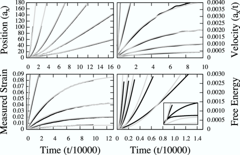
Figure 10: Additional comparisons between simulation data (black lines) and viscous motion equations (gray lines) for glide where where $M_{\gamma}$ is the only adjustable parameter. From left to right in each plot curves are shown for $\dot{\gamma}=2\times 10^{-5}$, $6\times 10^{-6}$, $2\times 10^{-6}$, $1\times 10^{-6}$, $5\times 10^{-7}$, and $2\times 10^{-7}/t$ except for the lower right which shows data for $\dot{\gamma}=2\times 10^{-4}$, $1.2\times 10^{-4}$, $8\times 10^{-5}$, $4\times 10^{-5}$, and $2\times 10^{-5}/t$. The inset in the lower right corner of the lower right plot shows data for lower shear rates, $\dot{\gamma}=6\times 10^{-6}$, $2\times 10^{-6}$, and $5\times 10^{-7}/t$ where Eq. (24) begins to fail. In all plots $r=-0.8$ and ($L_{x},L_{y}$)=(56,46).

It is worth examining the strain dependence of the velocity further. In gradient systems, the velocity of finite structures is expected to be proportional to the driving force applied $F_{D}$, which in this case can be interpreted as the derivative of the change in free energy due to the application of shear;

$$v\sim F_{D}=\frac{d\Delta F_{Shear}}{d\bar{\gamma}}\simeq\frac{q_{eq}^{4}A^{2}}{3}\bar{\gamma}.$$ (25)

Additionally, Eqs. (15)–(23) indicate that velocity is in general linear in $\bar{\gamma}$ for this type of overdamped system. All simulations resulted in approximately linear velocity ($v$) vs. $\bar{\gamma}$ behavior for dislocation glide, as shown in Fig. 11. It is important to correct the overall strain shown in Fig. 11 for that relieved by the glide of the dislocation (Eq. (13)), especially when using small system sizes.

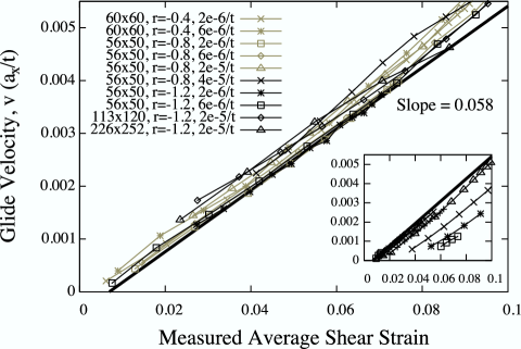
Figure 11: Dislocation glide velocity under rigid displacement as a function of the measured average shear strain, $\bar{\gamma}$. A number of system sizes, temperatures, and shear rates are shown to illustrate the uniformity of the dynamics. The heavy line is a representative linear fit. Inset: Dislocation glide velocity under relaxational displacement at various shear rates and two values of $r$. The strain values are overestimated due to the nonlinear shear profile produced by this type of shearing, but the slopes are relatively unchanged. The heavy line is the same linear fit as in the larger graph.

Both methods of displacement produce nearly the same value of $M_{\gamma}$ under all conditions, though it is more difficult to determine the local strain around the dislocation for the case of relaxational displacement, due to the nonlinear shear profile. For rigid displacement, the free energy follows the expected form ($\Delta F_{Shear}\sim\bar{\gamma}^{2}$) and the velocity appears to be linear for $\bar{\gamma}$ less than $\sim 10$%. For relaxational displacement, the anomaly in the free energy behavior noted above complicates the results, but the velocity remains linear in $\bar{\gamma}$ with values of $M_{\gamma}$ similar to those found for rigid displacement. An analytic calculation of $M_{\gamma}$ would complete this analysis of the dynamics, but since the simulation results indicate no strong dependencies on any variables, $M_{\gamma}=0.06a_{x}/t$ is believed to be a reasonable estimate for most cases of interest.

Shear was also applied along directions not lying on one of the axes of symmetry with predictable results. As the angle $\theta_{R}$ is increased (with $0^{\circ}$ denoting alignment with a symmetry axis), the Peierls barrier grows but the slip direction remains along the nearest symmetry axis. Once $\theta_{R}$ becomes large enough, approximately $10-30^{\circ}$ depending on the value of $r$, the dislocation prefers to climb rather than glide, with motion in the general direction of the applied shear.

A similar analysis to that presented in Eqs. (15)–(24) can be applied to the case of constant strain by removing the external force from Eq. (15). The resulting equations were also found to agree well with simulation data. It is also worth noting that the velocity vs. $\bar{\gamma}$ behavior is essentially the same as that shown in Fig. 11 when the shear condition is one of constant strain.

III.3 Climb: Constant Applied Strain Rate Dynamics

Climb simulations were conducted using steady compression over a range of parameter values similar to those used for glide simulations. Before presenting the results, a caveat on this portion of the study is in order. It was found that the results varied systematically (i.e. the Peierls barrier decreased) with the grid spacing $\Delta x$, apparently due to the decrease in relevant dimensions with compression. A grid spacing small enough to overcome this effect could not be reached since the time step must be dramatically decreased with $\Delta x$. But the nature of the results and the essential physics remain the same; the data is only shifted by this effect. An example of the climb simulation geometry is shown in Fig. 12.

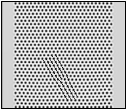
Figure 12: A small sample climb simulation setup where $\rho(x,y)$ has been plotted. The extra row of particles terminating at the core of the dislocation has been highlighted.

III.3.1 Peierls Barrier for Climb

The dependence of $\epsilon_{P}$ on $\rho_{d}$ is of the same nature as that found for $\gamma_{P}$. No change was found under rigid displacement as $L_{x}$ and $L_{y}$ were increased, but an increase with $L_{x}$ was observed under relaxational displacement, again in proportion to the diffusion time from the edge of the sample to the dislocation core.

The $r$ dependence of $\epsilon_{P}$ is shown in Fig. 13 for various strain rates. Comparison with the glide Peierls barrier data in Fig. 7 confirms the same general linear behavior. $\epsilon_{P}$ is quite large at low $r$ but decreases toward $T_{c}$ such that there is a crossover close to $T_{c}$ where $\epsilon_{P}$ becomes less than $\gamma_{P}$. Thus climb is predominant at high temperatures, in agreement with the accepted phenomenology dd90 . This was also confirmed in the glide simulations where climb was found be preferred near $T_{c}$, even at very low values of applied shear. Note that the data shown in Fig. 13 was obtained using modified boundary conditions of mirror on all sides with no liquid phase.

Following ken04 , the change in $F$ under compression can be calculated by substituting $\rho(x/(1+\bar{\epsilon}),y)$ into Eq. (1) and minimizing with respect to $A$. The result is similar to that for shear;

$$\Delta F_{Comp.}=\frac{q^{4}_{eq}A^{2}}{2}\bar{\epsilon}^{2}.$$ (26)

In this limit, as was also the case for glide, $\epsilon_{P}$ can be written in the form

$$\epsilon_{P}=\sqrt{\frac{2\Delta F_{P}^{Climb}(\rho_{0},r)}{q^{4}_{eq}A^{2}}}.$$ (27)

Figure 13: Temperature dependence of the Peierls strain barrier for climb without thermal fluctuations. Data shown is at $\rho_{0}=0.25$ and ($L_{x},L_{y}$)=(52,103) under rigid displacement.

The strain rate dependence is also similar to that for glide, as shown more clearly in Fig. 14. The results show that $\gamma_{P}\sim\dot{\gamma}^{0.30}$, which is similar to the dependence $\gamma_{P}\sim\dot{\gamma}^{0.37}$ measured for glide at the same $r$. The absolute values of $\epsilon_{P}$ are significantly higher than those for glide in this case because of the low value of $r$ that was used. The same arguments leading to Eq. (9) should apply to climb as well, since the behavior seems to be essentially the same as that found for glide.

Figure 14: Measured Peierls strain barrier for climb and the subsequent mobilities under rigid displacement at $r=-1.2$ and ($L_{x},L_{y}$)=($52,166$).

III.3.2 Atomistic Climb Mechanism

Dislocation climb is a nonconservative process. It requires either the diffusion of particles away from the dislocation core or toward it, unlike glide which involves only rearrangements of particles around the core. The mechanism of climb is shown in Fig. 15, where in these simulations mass diffuses away from the core since the strain is applied through compression.

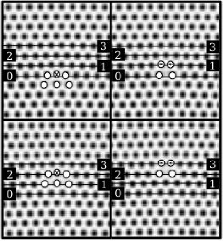
Figure 15: Atomistic climb mechanism under constant applied strain rate. From top left to bottom right, $\rho(x,y)$ is shown at $t$=300, 600, 800, and 900, corresponding to $\bar{\epsilon}$=2.4$\%$, 4.8$\%$, 6.4$\%$, and 7.2$\%$. The particles around the dislocation core have been highlighted and the rows near the core have been labeled for clarity. The particles marked with an ’X’ are those which diffuse away between subsequent images, and those marked with arrows merge together.

Again, similar to what was found for glide, the motion has a stick-slip character at low velocities and becomes more continuous at higher velocities. The motion proceeds by alternating between configurations 1 and 2 (Fig. 4). Starting from Config. 2, as shown in the upper left image of Fig. 15, the particle marked with an ’X’ diffuses away, leaving the core in Config. 1 as shown in the next image. The two particles marked with arrows then merge together, returning the dislocation to Config. 2 as shown in the subsequent image. The process repeats as long as there is sufficient strain energy to maintain motion. For climb in the opposite direction, particles diffuse in and split rather then diffuse away and merge, respectively. This merging and splitting of particles may seem unphysical, but in a time-averaged sense these motions simply represent diffusion of mass away from or toward the dislocation core, which is the fundamental limiting process in dislocation climb.

III.3.3 Viscous Dynamics

The dynamics of a single climbing dislocation are well described by the same damped equation of motion used to describe glide (Eq. (15)). Again, the only adjustable parameter is $M_{\epsilon}$, the effective mobility for dislocation climb. Fig. 16 shows the agreement between these analytic results and typical sets of simulation data.

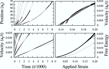
Figure 16: Comparisons between simulation data (black lines) and viscous motion equations (gray lines) for climb. From left to right in each plot curves are shown for $\dot{\epsilon}=2\times 10^{-4}$, $1.2\times 10^{-4}$, $8\times 10^{-5}$, $4\times 10^{-5}$, $2\times 10^{-5}$, and $6\times 10^{-6}/t$. In all plots $r=-1.2$ and ($L_{x},L_{y}$)=(52,166).

The velocity versus $\bar{\epsilon}$ behavior shown in Fig. 16 appears to be slightly nonlinear, but this is due to the relatively short range of motion that could be captured with computationally tractable system sizes. An approximate $M_{\epsilon}$ can nonetheless be extracted, and the results indicate first of all that the values of $M_{\epsilon}$ are an order of magnitude higher than those measured for $M_{\gamma}$ ($M_{\epsilon}\simeq 0.5$). The slopes of the $v$ versus $\bar{\epsilon}$ curves are much steeper for climb than for glide, but at the same time the velocities remain zero to much higher strains due to the larger values of $\epsilon_{P}$ (except near $T_{c}$). Also, $M_{\epsilon}$ is not quite as unchanging as $M_{\gamma}$, in that relatively weak, though measurable dependencies on $r$ and $\dot{\epsilon}$ were found. The data indicates a slight decrease in $M_{\epsilon}$ with increasing $r$ and an increase with $\dot{\epsilon}$ that goes like $\sqrt{\dot{\epsilon}}$ (Fig. 14).

To calculate the dynamics of $F$, Eq. (23) can be substituted into Eq. (26) to give

$$\Delta F_{Comp.}=\frac{1}{2}\bigg{[}\frac{q^{2}_{eq}A\dot{\epsilon}}{M_{\epsilon}\rho_{d}b}\big{(}1-e^{-M_{\epsilon}\rho_{d}bt}\big{)}\bigg{]}^{2}$$ (28)

which agrees reasonably well with the data shown in Fig. 16. The difference is mostly due to the low value of $r$ used, since the one mode approximation loses accuracy away from $T_{c}$. No anomaly in $F$ like that found in the glide data was observed in the climb simulations. All curves of the change in $F$ under compression fall onto approximately the same curve when plotted versus $\bar{\epsilon}$.

Compression was also applied along directions not lying on one of the axes of symmetry at $r=-0.8$. As the angle $\theta_{R}$ is increased, the dislocation first glides some distance proportional to $\theta_{R}$ in a direction along the nearest symmetry axis. Then climb begins along the same lattice direction as in the unrotated case, with the value of $\epsilon_{P}$ increasing only slightly with $\theta_{R}$. Nearer $T_{c}$ it would be reasonable to expect less tendency toward the initial gliding, as climb becomes the preferred type of motion. Generally speaking, the application of strain along irregular directions relative to the lattice symmetry results in a mixed motion of glide and climb.

III.4 Annihilation

Annihilation occurs when two dislocations having opposite burger’s vectors merge and eliminate each other. There exists a critical separation, $r_{c}$, at a given angle, $\theta_{0}$, below which annihilation will occur, and this separation is in principle a function of the crystal symmetry, type of dislocation, temperature, relative velocity, and the local strain field. Results were obtained here for the static case ($v=0$) at a single temperature and under no applied strain, for two perfect edge dislocations.

Consider one dislocation at some location $(0,0)$ and another at $(d_{x},d_{y})$ with opposite burger’s vector. In radial coordinates the separation can be expressed in terms of a distance $r_{0}$ and an angle $\theta_{0}$. At $\theta_{0}=0^{\circ}$, annihilation occurs by pure glide, and as $\theta_{0}$ is increased a mixed motion of glide and climb is required, until $\theta_{0}=90^{\circ}$ where annihilation occurs by pure climb. $r_{c}$ was determined as a function of $\theta_{0}$ by increasing the initial separation until annihilation no longer occurred. Periodic boundary conditions were used in all directions and the parameters chosen were $\rho_{0}=0.25$, $r=-0.25$, and $(L_{x},L_{y})=(56,43)$. The equilibrium wavenumber at this $\rho_{0}$ and $r$ would require 56.5 particles in the $x-$direction, so placing 56/row in the bottom half and 57/row in the top half produces a dislocation with no preset bias toward climb in either direction. The results are shown in Fig. 17.

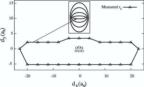
Figure 17: Measured critical radii for annihilation at $r=-0.25$ and $\rho_{0}=0.25$. The configuration shown in the center is the reference dislocation at $(0,0)$ from which $\theta_{0}$ was measured. The inset shows a schematic of the expected behavior as the temperature is increased above the crossover $r$ at which climb becomes dominant.

Despite the unbiasing, $r_{c}$ is asymmetric with a preference toward climb in the $-y$ direction. This is apparently a consequence of the asymmetry of the strain field across the $x-$axis of the dislocation core, where there is an enhancement of strain in the lower half-plane. The particle positions around the core clearly reflect this asymmetry. Note that the details of the strain field will be slightly different for a dislocation in Config. 1, but the same argument should nonetheless hold.

The elliptical shape of $r_{c}(\theta_{0})$ is expected since $\gamma_{P}^{0}<\epsilon_{P}^{0}$ for this parameter set. As $r$ is increased, eventually $\epsilon_{P}^{0}<\gamma_{P}^{0}$, and the primary axis of the ellipse should coincide with the $y-$axis (climb axis), becoming more elliptical as $T_{c}$ is approached. This expected behavior is shown schematically in the inset of Fig. 17. Moving from the inner to the outer ellipse corresponds to increasing $r$.

Extending the elliptical approximation and assuming that $r_{c}$ is directly proportional to the Peierls strain, one can write a temperature dependent equation for $r_{c}$;

$$r_{c}(\theta_{0},r)\simeq\frac{|A_{\gamma}A_{\epsilon}r|}{\sqrt{A_{\gamma}^{2}\sin^{2}{\theta_{0}}+A_{\epsilon}^{2}\cos^{2}{\theta_{0}}}}$$ (29)

where $A_{\gamma}$ and $A_{\epsilon}$ are the slopes of the Peierls strain versus $r$ curves for glide and climb respectively.

IV Conclusion

Three fundamental dislocation processes have been numerically examined in idealized two dimensional settings using a phenomenological PFC model. The diffusive dynamics were measured over a range of temperatures, dislocation densities, and experimentally accessible strain rates. In equilibrium, two stable edge dislocation configurations were found to exist, with one resulting in a slightly lower Peierls barrier for glide than the other. The Peierls barriers for glide and climb, $\gamma_{P}$ and $\epsilon_{P}$ respectively, were found to have little or no dependence on dislocation density, and both showed approximately linear decreases with increasing temperature (in the absence of thermal fluctuations). Near $T_{c}$, $\epsilon_{P}<\gamma_{P}$ verifying the expectation that climb is dominant at high temperatures. A crossover temperature was identified below which $\gamma_{P}<\epsilon_{P}$ and glide becomes the preferred type of motion. Both strain barriers also showed essentially power law increases with the applied strain rate, where the exponents are similar for glide and climb at equal $r$’s. Under relaxational displacement (no phonons), $\gamma_{P}$ is nearly linear in $\dot{\gamma}$ and goes as Eq. (9), while under rigid displacement at high strain rates (strong phonons) the deviation from linear is much greater ($\gamma_{P}\simeq\dot{\gamma}^{0.38}$) with relatively little change in the barrier strain at high strain rates. Physical arguments and some mathematical arguments were given for all of these behaviors.

Rigid displacement with $\dot{\gamma},\dot{\epsilon}>5\times 10^{-6}/t$ most accurately reproduces the rigid behavior of a real crystal. A more rigorous PFC model, derived from microscopics, that will include a wave term to simulate phonon dynamics is currently being developed mpfc . Based on the results presented here, it is expected that this model will produce dynamics that fall between the limits of relaxational and rigid response. At strain rates below approximately $2\times 10^{-7}/t$, the two methods of displacement are essentially equivalent.

The motion of a gliding or climbing edge dislocation was found to be stick-slip in character at low velocities and nearly continuous at high velocities. Three possible regimes of motion were observed for glide, depending on the expected steady-state velocity of the dislocation defined in Eq. (12). These involve an oscillatory glide, a steady-state glide, and slipping rows of particles, in order of increasing $v_{ss}$.

A simple viscous dynamic model has been formulated to describe the results obtained for gliding and climbing dislocations, where the only adjustable parameter is $M_{\gamma}$ or $M_{\epsilon}$. Excellent agreement is obtained between these equations and the simulation results, both of which indicate that velocity is linear in strain for both glide and climb. The slope of the $v$ versus $\bar{\gamma}$ curve for glide, $M_{\gamma}$ was found to be nearly unchanging across all parameter ranges. The slope for climb, $M_{\epsilon}$, which is an order of magnitude greater than $M_{\gamma}$, was found to increase approximately as $\sqrt{\dot{\epsilon}}$.

A critical distance for the annihilation of two edge dislocations was also measured, and an asymmetry with preference toward annihilation in the $-y$ direction was found. $r_{c}(\theta_{0})$ approximately takes the form of an ellipse whose major axis is predicted to be along the glide direction at low temperatures and along the climb direction at high temperatures.

Other phase-field models have recently been used to study dislocation dynamics cuitino01 ; koslowski02 ; wang01b ; wang05 . These approaches differ from the PFC method in that they do not naturally contain atomistic detail. The domains in these models typically differentiate dislocation loops and the interfaces represent dislocation lines. Coarsening of large arrays of lines etc. can be efficiently studied, but atomistic detail is either lost or must be explicitly added through postulated Peierls potentials. The relevant equations of elasticity must also be rigorously applied, unlike in the PFC model which naturally exhibits elastic behavior as well as Peierls potentials.

Other phenomena relevant to dislocation dynamics, such as obstacle and impurity effects, could be studied with a similar approach, and more complicated dynamics involving screw dislocations, dislocation loops, multiplication processes, etc. could be examined in three dimensional simulations. Alternatively, the two dimensional model could provide interesting insights into the problem of dislocation-mediated melting in two dimensions.

- (1) J. Chang, V. V. Bulatov, and S. Yip. J. Computer-Aided Materials Design, 6:165, 1999.
- (2) J. Chang, W. Cai, V. V. Bulatov, and S. Yip. Comp. Mat. Sci., 23:111–115, 2002.
- (3) N. P. Bailey, J. P. Sethna, and C. R. Myers. Mat. Sci. & Eng. A, 309-310:152–155, 2001.
- (4) E. Rodary, D. Rodney, L. Proville, Y Bréchet, and G. Martin. Phys. Rev. B, 70:054111, 2004.
- (5) R. J. Amodeo and N. M. Ghoniem. Phys. Rev. B, 41(10):6958, 1990.
- (6) V. V. Bulatov, F. F. Abraham, L. Kubin, B. Devincre, and S. Yip. Nature, 391:669, 1998.
- (7) N. Goldenfeld, B. P. Athreya, and J. A. Dantzig. Phys. Rev. E, 72:020601(R), 2005.
- (8) F. Pardo, F. de la Cruz, P. L. Gammel, E. Bucher, and D. J. Bishop. Nature (London), 396:348, 1998.
- (9) C. Sagui and R. C. Desai. Phys. Rev. E, 52:2807, 1995.
- (10) D. Orlikowski, C. Sagui, A. Somoza, and C. Roland. Phys. Rev. B, 59:8646, 1999.
- (11) C. Harrison, H. Adamson, Z. Cheng, J. M. Sebastian, S. Sethuraman, D. A. Huse, R. A. Register, and P. M. Chaikin. Science, 290:1558, 2000.
- (12) M. Laradji, H. Guo, M. Grant, and M. J. Zuckermann. Phys. Rev. A, 44:8184, 1991.
- (13) K. R. Elder, M. Katakowski, M. Haataja, and M. Grant. Phys. Rev. Lett., 88:245701, 2002.
- (14) Y. Oono and S. Puri. Phys. Rev. A, 38:434–453, 1988.
- (15) R. Phillips. Crystals, defects and microstructures: Modeling across scales. pages 406–412, 2001.
- (16) W. Wasserbäch. Phil. Mag., A53:335, 1986.
- (17) R. Lachenmann and H. Schultz. Scripta Metall., 4:33, 1970.
- (18) A. M. Cuitino, L. Stainier, G. Wang, A. Strachan, T. Cagin, W. Goddard III, and M. Ortiz. Caltech Tech. Report., 112, 2001.
- (19) M. Tang, B. Devincre, and L. P. Kubin. Mod. and Sim. in Mat. Sci. and Eng., 7:893, 1999.
- (20) K. R. Elder and M. Grant. Phys. Rev. E, 70:051605, 2004.
- (21) T. C. Lubensky, S. Ramaswamy, and J. Toner. Phys. Rev. B, 32:7444–7452, 1985.
- (22) P. Stefanovic, M. Haataja, S. Majaniemi, and N. Provatas. to be published, 2005.
- (23) M. Koslowski, A. M. Cuitino, and M. Ortiz. J. Mech. Phys. of Solids, 50:2597, 2002.
- (24) Y. U. Wang, Y. M. Jin, A. M. Cuitino, and A. G. Khachaturyan. Appl. Phys. Lett., 78:2324–2326, 2001.
- (25) Y. U. Wang, Y. M. Jin, and A. G. Khachaturyan. Phil. Mag., 85:261–277, 2005.