Spin Decay in a Quantum Dot Coupled to a Quantum Point Contact

Abstract

We consider a mechanism of spin decay for an electron spin in a quantum dot due to coupling to a nearby quantum point contact (QPC) with and without an applied bias voltage. The coupling of spin to charge is induced by the spin-orbit interaction in the presence of a magnetic field. We perform a microscopic calculation of the effective Hamiltonian coupling constants to obtain the QPC-induced spin relaxation and decoherence rates in a realistic system. This rate is shown to be proportional to the shot noise of the QPC in the regime of large bias voltage and scales as $a^{-6}$ where $a$ is the distance between the quantum dot and the QPC. We find that, for some specific orientations of the setup with respect to the crystallographic axes, the QPC-induced spin relaxation and decoherence rates vanish, while the charge sensitivity of the QPC is not changed. This result can be used in experiments to minimize QPC-induced spin decay in read-out schemes.

I Introduction

Recent progress in nanotechnology has enabled access to the electron spin in semiconductors in unprecedented ways, ALS ; WolfScience ; DasSarma with the electron spin in quantum dots being a promising candidate for a qubit due to the potentially long decoherence time of the spin.LD ; Vero Full understanding of the decoherence processes of the electron spin is thus crucial. On the other hand, as a part of a quantum computer, read-out systems play an essential role in determining the final result of a quantum computation. However, read-out devices, in general, affect the spin state of the system in an undesired way. Quantum point contacts (QPCs) which are used as charge detectors,Buks in particular, couple to the spin via the spin-orbit interaction. For small GaAs quantum dots, the spin-orbit length ($\lambda_{SO}\approx 8\;\mu$m) is much larger than the dot size ($\lambda_{d}\approx 50$ nm) and thus the spin-orbit interaction presents a small perturbation. Nevertheless, we will see that shot noise in the QPC can induce an appreciable spin decay via this weak spin-orbit coupling.

Quite remarkably, the number of electrons in quantum dots can be tuned starting from zero. Tarucha ; Ciorga ; Elzerman ; PettaPRL More recently, Zeeman levels have been resolved Hanson and the spin relaxation time ($T_{1}$) has been measured, yielding times of the order of milliseconds in the presence of an in-plane magnetic field of $8$ T.ENature ; HansonCM In these experiments, based on spin-charge conversion,LD use is made of a QPC located near the quantum dot as a sensitive charge detector to monitor changes of the number of electrons in the dot. The shot noise in the QPC affects the electron charge in the quantum dot via the Coulomb interaction,Buks ; Field and therefore, it can couple to the electron spin as well, via the spin-orbit interaction. While charge relaxation and decoherence in a quantum dot due to a nearby functioning QPC have been studied before,Levinson ; Aleiner we show here that the same charge fluctuations in the QPC introduce spin decay via spin-orbit and Zeeman interactions. Note that several read-out schemes utilizing a QPC have been considered beforenshot in the context of the spin qubit. However, in Ref. nshot, the QPC was used for charge read-out, while the spin state of the qubit was converted into the charge state of a reference dot.LD Recently, a different read-out scheme has been implemented,ENature in which the reference dot was replaced by a Fermi lead and the QPC was coupled directly to the spin qubit.

The effect of spin-orbit interaction on spin relaxation and decoherence was considered in Ref. GKL, . There, it was shown that the decoherence time $T_{2}$ due to spin-orbit interaction approaches its upper bound,GKL i.e. $T_{2}=2T_{1}$, determined by spin-flip processes.GKL ; KhaNaz Measurements of $T_{1}$ have been performed on spins in electrostatically confined (lateral) quantum dotsENature ($T_{1}\simeq 0.85\,{\rm ms}$) and self-assembled quantum dotsKroutvar ($T_{1}\simeq 20\,{\rm ms}$). The measured spin relaxation times $T_{1}$ in both cases agree well with the theory in Refs. GKL, and KhaNaz, . In addition to the spin-orbit interaction, the hyperfine interaction plays an important role in quantum dots. BLD ; KhaetskiiLossGlazman ; MerculovEfrosRosen ; ErlingssonNazarov ; SchliemannKhaetskiiLossNUCL ; SousaDasSarma ; Bill ; Bracker ; Koppens ; PettaT2Nature ; PettaScience Measurements of the spin decoherence time $T_{2}$ have recently been performed in a self-assembled quantum dotBracker ($T_{2}^{*}\simeq 16\,{\rm ns}$) as well as in a double-dot setup for singlet-triplet decoherence ($T_{2}\simeq 10\,{\rm\mu s}$).PettaScience Finally we note that a number of alternative schemes to measure the decoherence time of the electron spin in quantum dots have been proposed.Engel ; GLA ; Gywat

Motivated by these recent experiments, we study here the effect of the QPC on spin relaxation and decoherence in the quantum dot. For this, we first derive an effective Hamiltonian for the spin dynamics in the quantum dot and find a transverse (with respect to the external magnetic field) fluctuating magnetic field. We calculate microscopically the coupling constants of the effective Hamiltonian by modeling the QPC as a one-dimensional channel with a tunnel barrier. We show that this read-out system speeds up the spin decay and derive an expression for the spin relaxation time $T_{1}$. However, there are some regimes in which this effect vanishes, in the first order of spin-orbit interaction. The relaxation time will turn out to be strongly dependent on the QPC orientation on the substrate, the distance between the QPC and the quantum dot, the direction of the applied magnetic field, the Zeeman splitting $E_{Z}$, the QPC transmission coefficient ${\cal T}$, and the screening length $\lambda_{sc}$ (see Fig. 1). Although this effect is, generally, not larger than other spin decay mechanisms (e.g. coupling of spin to phonons GKL or nuclear spins Bill ), it is still measurable with the current setups under certain conditions. The following results could be of interest to experimentalists to minimize spin decay induced by QPC-based charge detectors.

The paper is organized as follows. In Section II we introduce our model for a quantum dot coupled to a quantum point contact and the corresponding Hamiltonian. Section III is devoted to the derivation of the effective Hamiltonian for the electron spin in the quantum dot. In Section IV we derive microscopic expressions for the coupling constants of the effective Hamiltonian and discuss different regimes of interest. Finally, in Section V, we calculate the electron spin relaxation time $T_{1}$ due to the QPC and make numerical predictions for typical lateral quantum dots.

II The Model

We consider an electron in a quantum dot and a nearby functioning quantum point contact (QPC), see Fig. 1, embedded in a two-dimensional electron gas (2DEG). We model the QPC as a one-dimensional wire coupled via the Coulomb interaction to the electron in the quantum dot. We also assume that there is only one electron inside the dot, which is feasible experimentally. Tarucha ; Ciorga ; Elzerman ; PettaPRL ; Hanson ; ENature The Hamiltonian describing this coupled system reads $H=H_{d}+H_{Z}+H_{SO}+H_{Q}+H_{Qd}$, where

$$H_{d} = \frac{p^{2}}{2m^{*}}+U(\bm{r}),$$ (1)

$$H_{Z} = \frac{1}{2}g\mu_{B}{{\bm{B}}}\cdot{{\bm{\sigma}}}=\frac{1}{2}E_{Z}{{\bm{n}}}\cdot{\bm{\sigma}},$$ (2)

$$H_{SO} = \beta(-p_{x}\sigma_{x}+p_{y}\sigma_{y})+\alpha(p_{x}\sigma_{y}-p_{y}\sigma_{x}),$$ (3)

$$H_{Q} = \sum_{lk\sigma}\epsilon_{k}\bar{C}^{\dagger}_{lk\sigma}\bar{C}_{lk\sigma},$$ (4)

$$H_{Qd} = \sum_{ll^{\prime}kk^{\prime}\sigma}\eta_{ll^{\prime}}({\bm{r}})\bar{C}^{\dagger}_{lk\sigma}\bar{C}_{l^{\prime}k^{\prime}\sigma}.$$ (5)

Here, $Q$ refers to the QPC and $d$ to the dot, ${\bm{p}}=-i\hbar{\bm{\nabla}}+(e/c)\bm{A}(\bm{r})$ is the electron 2D momentum, $U(\bm{r})$ is the lateral confining potential, with ${\bm{r}}=(x,y)$, $m^{*}$ is the effective mass of the electron, and $\bm{\sigma}$ are the Pauli matrices. The 2DEG is perpendicular to the $z$ direction. The spin-orbit Hamiltonian $H_{SO}$ in Eq.(3) includes both Rashba Rashba spin-orbit coupling ($\alpha$), due to asymmetry of the quantum well profile in the $z$ direction, and Dresselhaus Dress spin-orbit couplings ($\beta$), due to the inversion asymmetry of the GaAs lattice. The Zeeman interaction $H_{Z}$ in Eq. (2) introduces a spin quantization axis along ${{\bm{n}}}={{\bm{B}}}/B=(\cos\varphi\sin\vartheta,\sin\varphi\sin\vartheta,\cos\vartheta)$. The QPC consists of two Fermi liquid leads coupled via a tunnel barrier and is described by the Hamiltonian $H_{Q}$, where $\bar{C}_{lk\sigma}^{\dagger}$, with $l=L,R$, creates an electron incident from lead $l$, with wave vector $k$ and spin $\sigma$. We use the overbar on, e.g., $\bar{C}_{lk\sigma}$ to denote the scattering states in the absence of electron on the dot. The Hamiltonian $H_{Qd}$ in Eq. (5) describes the coupling between the quantum dot electron and the QPC electrons. We assume that the coupling is given by the screened Coulomb interaction,

$$\eta_{ll^{\prime}}({\bm{r}}) = \langle\overline{lk}|\frac{e^{2}}{\kappa|{\bm{r}}-{\bm{R}}|}\tilde{\delta}({\bm{R}}-{\bm{a}})|\overline{l^{\prime}k^{\prime}}\rangle,$$ (6)

where ${\bm{R}}=(X,Y)$ is the coordinate of the electron in the QPC and $\kappa$ is the dielectric constant. The Coulomb interaction is modulated by a dimensionless screening factor $\tilde{\delta}({\bm{R}}-{\bm{a}})$, where ${\bm{a}}=(0,a)$ gives the QPC position (see Fig. 1). The quantum dot electron interacts with the QPC electrons mostly at the tunnel barrier; away from the tunnel barrier the interaction is screened due to a large concentration of electrons in the leads. For the screening factor we assume, in general, a function which is peaked at the QPC and has a width $2\lambda_{sc}$ (see Fig. 1). Note that $\lambda_{sc}$ is generally different from the screening length in the 2DEG and depends strongly on the QPC geometry and size. Generally, $\eta_{ll^{\prime}}$ are $k$-dependent, however, their $k$-dependence turns out to be weak and will be discussed later.

Figure 1: Schematic of the quantum dot (QD) coupled to a QPC. The $(X,Y)$ frame gives the setup orientation, left (L) and right (R) leads, with respect to the crystallographic directions $x^{\prime}\equiv[110]$ and $y^{\prime}\equiv[\bar{1}10]$. The dot has a radius $\lambda_{d}$ and is located at a distance $a$ from the QPC. The vector ${\bm{R}}$ describes the QPC electrons and ${\bm{r}}$ refers to the coordinate of the electron in the dot. The noise of the QPC current $I$ perturbs the electron spin on the dot via the spin-orbit interaction.

III The Effective Hamiltonian

The quantum dot electron spin couples to charge fluctuations in the QPC via the spin-orbit Hamiltonian (3). The charge fluctuations are caused by electrons passing through the QPC. To derive an effective Hamiltonian for the coupling of spin to charge fluctuations, we perform a Schrieffer-Wolff transformation,Mahan $\tilde{H}=\exp(S)H\exp(-S)$, and remove the spin-orbit Hamiltonian in leading order. We thus require that $\left[H_{d}+H_{Z},S\right]=H_{SO}$, under the condition $\lambda_{d}\ll\lambda_{SO}$, where $\lambda_{d}$ is the quantum dot size and $\lambda_{SO}=\hbar/m^{*}(|\beta|+|\alpha|)$ is the minimum spin-orbit length. The transformed Hamiltonian is then given by

$$\tilde{H} = H_{d}+H_{Z}+H_{Q}+H_{Qd}+\left[S,H_{Qd}\right],$$ (7)

$$S = \frac{1}{L_{d}+L_{Z}}H_{SO}=\frac{1}{L_{d}}\sum_{m=0}^{\infty}\left(-L_{Z}\frac{1}{L_{d}}\right)^{m}H_{SO},\;\;\;\;\;$$ (8)

$$H_{SO} = iL_{d}({\bm{\sigma}}\cdot{\bm{\xi}}),$$ (9)

where $L$ is Liouville superoperator for a given Hamiltonian defined by $LA\equiv[H,A]$ and ${\bm{\xi}}$ is a vector in the 2DEG plane and has a simple form in the coordinate frame $x^{\prime}=(x+y)/\sqrt{2}$, $y^{\prime}=(y-x)/\sqrt{2}$, $z^{\prime}=z$, namely, ${\bm{\xi}}=(y^{\prime}/\lambda_{-},x^{\prime}/\lambda_{+},0)$, where $\lambda_{\pm}=\hbar/m^{*}(\beta\pm\alpha)$ are the spin-orbit lengths. For a harmonic dot confinement $U(r)=\frac{1}{2}m^{*}\omega_{0}^{2}r^{2}$, we have

$$\frac{1}{L_{d}}x = \frac{-i}{\hbar m^{*}\omega_{0}^{2}}\left(p_{x}+\frac{eB_{z}}{c}y\right),$$ (10)

$$\frac{1}{L_{d}}y = \frac{-i}{\hbar m^{*}\omega_{0}^{2}}\left(p_{y}-\frac{eB_{z}}{c}x\right),$$ (11)

$$\frac{1}{L_{d}}p_{j} = \frac{im^{*}}{\hbar}r_{j},\;\;\;\;\;\;\;\;\;\;\;\;\;(j=x,y).$$ (12)

In addition, we have the following relations for the Zeeman Liouvillian

$$L^{m}_{Z}({\bm{\sigma}}\cdot{\bm{\xi}})=\left\{\begin{array}[]{l}\;\;iE_{Z}^{m}[{\bm{n}}\times{\bm{\xi}}]\cdot{\bm{\sigma}},\;\;\;\;\;\;\;\;\;\mbox{for odd }m>0\\ -E_{Z}^{m}[{\bm{n}}\times({\bm{n}}\times{\bm{\xi}})]\cdot{\bm{\sigma}},\;\;\;\mbox{for even }m>0,\end{array}\right.$$ (13)

where $E_{Z}=g\mu_{B}B$ is the Zeeman splitting. The last term in Eq. (7) gives the coupling of the dot spin to the QPC charge fluctuations. The transformation matrix $S$ (to first order in spin-orbit interaction) can be derived by using the above relations (see Appendix A). We obtain

$$-iS = \mbox{\boldmath$\xi$}\cdot\mbox{\boldmath$\sigma$}+\left[\mbox{\boldmath$n$}\times\mbox{\boldmath$\xi$}_{1}\right]\cdot\mbox{\boldmath$\sigma$}-\left[\mbox{\boldmath$n$}\times\left[\mbox{\boldmath$n$}\times\mbox{\boldmath$\xi$}_{2}\right]\right]\cdot\mbox{\boldmath$\sigma$},\;\;\;\;\;\;\;$$ (14)

$$\mbox{\boldmath$\xi$}_{1} = \left((\alpha_{1}p_{y^{\prime}}+\alpha_{2}x^{\prime})/\lambda_{-},\,(\alpha_{1}p_{x^{\prime}}-\alpha_{2}y^{\prime})/\lambda_{+},\,0\right),\;\;\;\;\;\;\;$$ (15)

$$\mbox{\boldmath$\xi$}_{2} = \left((\beta_{1}p_{x^{\prime}}+\beta_{2}y^{\prime})/\lambda_{-},\,(-\beta_{1}p_{y^{\prime}}+\beta_{2}x^{\prime})/\lambda_{+},\,0\right),\;\;\;\;\;\;\;$$ (16)

$$\alpha_{1} = \frac{\hbar}{m^{*}}\frac{E_{Z}[E_{Z}^{2}-(\hbar\omega_{0})^{2}]}{(E_{Z}^{2}-E_{+}^{2})(E_{Z}^{2}-E_{-}^{2})},$$ (17)

$$\alpha_{2} = \frac{E_{Z}\hbar\omega_{c}(\hbar\omega_{0})^{2}}{(E_{Z}^{2}-E_{+}^{2})(E_{Z}^{2}-E_{-}^{2})},$$ (18)

$$\beta_{1} = \frac{\hbar}{m^{*}}\frac{E_{Z}^{2}\hbar\omega_{c}}{(E_{Z}^{2}-E_{+}^{2})(E_{Z}^{2}-E_{-}^{2})},$$ (19)

$$\beta_{2} = E_{Z}^{2}\frac{(\hbar\omega_{c})^{2}+(\hbar\omega_{0})^{2}-E_{Z}^{2}}{(E_{Z}^{2}-E_{+}^{2})(E_{Z}^{2}-E_{-}^{2})},$$ (20)

where $E_{\pm}=\hbar\omega\pm\hbar\omega_{c}/2$, with $\omega=\sqrt{\omega_{0}^{2}+\omega_{c}^{2}/4}$ and $\omega_{c}=eB_{z}/m^{*}c$. Here, we assume $E_{\pm}-|E_{Z}|\gg|E_{Z}\lambda_{d}/\lambda_{SO}|$, which ensures that the lowest two levels in the quantum dot have spin nature. Below, we consider low temperatures $T$ and bias $\Delta\mu$, such that $T,\Delta\mu\ll E_{\pm}-|E_{Z}|$, (hence only the orbital ground state is populated so that its Zeeman sublevels constitute a two level system) and average over the dot ground state in Eq. (7). We obtain, using Eqs. (10)-(13), the following effective spin Hamiltonian

$$H_{\rm eff}=\frac{1}{2}g\mu_{B}\left[{{\bm{B}}}+\delta{{\bm{B}}}(t)\right]\cdot{{\bm{\sigma}}},$$ (21)

and the effective fluctuating magnetic field $\delta{{\bm{B}}}(t)$ is then given by the operator

$$\delta{{\bm{B}}}(t) = 2{\bm{B}}\times\left[{\bm{\Omega}}_{1}(t)+{\bm{n}}\times{\bm{\Omega}}_{2}(t)\right],$$ (22)

$${\bm{\Omega}}_{1} = \frac{e\hbar^{2}\gamma_{1}}{m^{*}}\left(\lambda_{-}^{-1}{\cal E}_{y^{\prime}},\lambda_{+}^{-1}{\cal E}_{x^{\prime}},0\right),$$

$${\bm{\Omega}}_{2} = \frac{e\hbar^{2}\gamma_{2}}{m^{*}}\left(-\lambda_{-}^{-1}{\cal E}_{x^{\prime}},\lambda_{+}^{-1}{\cal E}_{y^{\prime}},0\right),$$

$$\gamma_{1} = \frac{m^{*}}{\hbar E_{Z}}\alpha_{1}=\frac{E_{Z}^{2}-(\hbar\omega_{0})^{2}}{(E_{+}^{2}-E_{Z}^{2})(E_{-}^{2}-E_{Z}^{2})},$$

$$\gamma_{2} = \frac{m^{*}}{\hbar E_{Z}}\beta_{1}=\frac{E_{Z}\hbar\omega_{c}}{(E_{+}^{2}-E_{Z}^{2})(E_{-}^{2}-E_{Z}^{2})},$$

where we have gone to the interaction picture with respect to the lead Hamiltonian $H_{Q}^{\prime}=H_{Q}+{\langle H_{Qd}\rangle}_{d}$ and omitted a spin-independent part. Note that the coordinate-dependent part of $S$ drops out and thus $\alpha_{2}$, $\beta_{2}$ do not enter. Here and below, we use ${\langle\dots\rangle}_{d}$ to denote averaging over the dot ground state. Note that $H_{Q}^{\prime}$ describes the QPC, while it is electrostatically influenced by the quantum dot with one electron in the ground state. Obviously, $H_{Q}^{\prime}$ can be rewritten in the same form as $H_{Q}$ in Eq. (4), but with a different scattering phase in the scattering states. To denote the new scattering states, we omit the overbar sign in our notations. We have introduced an effective electric field operator $\mbox{\boldmath${\cal E}$}(t)$ in the interaction picture, Mahan

$$\mbox{\boldmath${\cal E}$}(t) = \frac{1}{e}{\langle{{\bm{\nabla}}}H_{Qd}(t)\rangle}_{d}$$ (23)

$$= \sum_{ll^{\prime}kk^{\prime}\sigma}\mbox{\boldmath${\varepsilon}$}_{ll^{\prime}}e^{i(\mu_{l}-\mu_{l^{\prime}})t/\hbar}C^{\dagger}_{lk\sigma}(t)C_{l^{\prime}k^{\prime}\sigma}(t),$$

$$\mbox{\boldmath${\varepsilon}$}_{ll^{\prime}} = \frac{1}{e}{\langle{{\bm{\nabla}}\eta_{ll^{\prime}}({\bm{r}})}\rangle}_{d},$$ (24)

where the fermionic operator $C_{l^{\prime}k^{\prime}\sigma}$ corresponds to scattering states in the leads with the dot being occupied by one electron ($H_{Q}^{\prime}$ is diagonal in $C_{l^{\prime}k^{\prime}\sigma}$). Here, $\mu_{l}$, $l=L,R$, are the chemical potentials of the left ($L$) and right ($R$) leads, with $\Delta\mu=\mu_{L}-\mu_{R}$ being the voltage bias applied to the QPC driving a current $I$. Note that in the absence of screening ($\tilde{\delta}({\bm{R}}-{\bm{a}})=1$ in Eq. (6)), ${\cal E}$ coincides with the electric field that the quantum dot electron exerts on the QPC electrons.

As a first result, we note that the fluctuating quantum field $\delta{{\bm{B}}}(t)$ is transverse with respect to the (classical) applied magnetic field ${{\bm{B}}}$ (cf. Ref. GKL, ). The magnetic field fluctuations originate here from orbital fluctuations that couple to the electron spin via the spin-orbit interaction. The absence of time reversal symmetry, which is removed by the Zeeman interaction, is crucial for this coupling. We assume no fluctuations in the external magnetic field ${{\bm{B}}}$. In our model, the dot electron spin couples to a bath of fermions, in contrast to Ref. GKL, where the bath (given by phonons) was bosonic.

To calculate the coupling constants $\mbox{\boldmath${\varepsilon}$}_{ll^{\prime}}$ in Eq. (23) , it is convenient to first integrate over the coordinates of the dot electron. We thus obtain $\mbox{\boldmath${\cal E}$}({\bm{R}})=\mbox{\boldmath${\cal E}$}_{0}({\bm{R}})\tilde{\delta}({\bm{R}}-{\bm{a}})$, see Eq. (6), where ${\bm{R}}$ refers to the location of the electrons in the QPC and the bare (unscreened) electric field is given by

$$\mbox{\boldmath${\cal E}$}_{0}({\bm{R}}) = {e\over\kappa}\left\langle\frac{{\bm{R}}-{\bm{r}}}{|{\bm{R}}-{\bm{r}}|^{3}}\right\rangle_{d}$$ (25)

$$= \frac{e{\bm{R}}}{\kappa R^{3}}\left(1+\frac{3}{4}\frac{\lambda_{d}^{2}}{R^{2}}+\dots\right).\;\;\;\;\;\;\;\;\;\;$$

Consequently, the coupling constants in Eq. (23) read $\mbox{\boldmath${\varepsilon}$}_{ll^{\prime}}=\langle lk|\mbox{\boldmath${\cal E}$}({\bm{R}})|l^{\prime}k^{\prime}\rangle$, where $|lk\rangle$ denote the scattering states in the leads. Here, we have assumed a parabolic confinement for the electron in the dot, set the origin of coordinates in the dot center (${\langle{\bm{r}}\rangle}_{d}=0$) and averaged with the dot wave function $\Psi_{d}({\bm{r}})=\exp{\left(-{r^{2}}/{2\lambda_{d}^{2}}\right)}/\lambda_{d}\sqrt{\pi}$, which is the ground state of the electron in a symmetric harmonic potential in two dimensions. While we choose a very special form for the ground state wave function, this does not affect substantially the final result, i.e. the relaxation time $T_{1}$. This is because any circularly symmetric wave function leads to the same form for $\mbox{\boldmath${\cal E}$}_{0}({\bm{R}})$ except that it just alters the second term in Eq. (25) which is very small compared to the first term (about one hundredth) and negligible. An analogous argument applies to asymmetric wave functions.

IV Coupling Constants ${\bm{\varepsilon}}_{ll^{\prime}}$

To proceed further, we construct the scattering states out of the exact wave functions of an electron in the QPC potential. While this is a generic method, we consider for simplicity a $\delta$-potential tunnel barrier for the QPC,

$$V(X)=\frac{\hbar^{2}b}{m^{*}}\delta(X),$$ (26)

where $b$ gives the strength of the delta potential. Then, the electron wave functions in the even and odd channels are given by

$$\psi_{e}(X) = \sqrt{2}\left\{\begin{array}[]{cc}\cos(kX+\phi),&X<0,\\ \cos(kX-\phi),&X>0,\end{array}\right.$$ (29)

$$\psi_{o}(X) = \sqrt{2}\sin kX,$$ (30)

where $\phi=\arctan(b/k)$, $k=\sqrt{2m^{*}E/\hbar^{2}}$ and, for convenience, the sample length is set to unity. Note that $\phi=\pi/2-\delta$, where $\delta\equiv\delta_{e}-\delta_{o}$ is the relative scattering phase between the even ($e$) and odd ($o$) channels. The transmission coefficient ${\cal T}$ through the QPC is related to $\phi$ by ${\cal T}(k)=\cos^{2}\phi$. We construct the scattering states in the following way

$$\left(\begin{array}[]{c}\psi^{L}_{\rm sc}\\ \psi^{R}_{\rm sc}\end{array}\right)={\cal U}\left(\begin{array}[]{c}\psi_{e}\\ \psi_{o}\end{array}\right),\;\;\;\;\;{\cal U}={-i\over{\sqrt{2}}}\left(\begin{array}[]{cc}e^{i\delta}&-1\\ e^{i\delta}&1\end{array}\right).$$ (37)

Up to a global phase, Eq. (37) is valid for any symmetric tunnel barrier.

IV.1 Three limiting cases

We calculate now the matrix elements of $\mbox{\boldmath${\cal E}$}({\bm{R}})$ using the wave functions (29) and (30). Three interesting regimes are studied in the following.

(i) $\lambda_{sc}\ll k_{F}^{-1}\ll a$, where $\lambda_{sc}$ is the screening length in the QPC leads and $k_{F}$ is the Fermi wave vector. In this case, we set $\tilde{\delta}({\bm{R}}-{\bm{a}})=2\lambda_{sc}\delta(X)$. By calculating the matrix elements of ${\varepsilon}$ with respect to the eigenstates of the potential barrier, Eqs. (29) and (30), we obtain

$$\mbox{\boldmath${\varepsilon}$}_{ee}=4\lambda_{sc}{\cal T}\mbox{\boldmath${\cal E}$}_{0}({\bm{a}}),\;\;\;\;\mbox{\boldmath${\varepsilon}$}_{oo}=\mbox{\boldmath${\varepsilon}$}_{eo}=0,$$ (38)

where we used the odd and even eigenstates and $\int dY|\Phi(Y)|^{2}\mbox{\boldmath${\cal E}$}(X,Y)=\mbox{\boldmath${\cal E}$}(X,a)$. Here, $\Phi(Y)$ is the QPC wave function in the transverse direction with width $\ll\lambda_{sc}$. Going to the Left-Right basis, Eq. (37), which is more suitable for studying transport phenomena, we obtain

$$\left(\begin{array}[]{cc}{\bm{\varepsilon}}_{LL}&{\bm{\varepsilon}}_{LR}\\ {\bm{\varepsilon}}_{RL}&{\bm{\varepsilon}}_{RR}\end{array}\right) = {1\over 2}{\bm{\varepsilon}}_{ee}\left(\begin{array}[]{cc}1&1\\ 1&1\end{array}\right).$$ (43)

Note that in this case we have ${\bm{\varepsilon}}_{ll^{\prime}}\propto{\cal T}$, where $l,l^{\prime}=L,R$, see Eqs. (38) and (43).

(ii) $k_{F}^{-1}\ll\lambda_{sc}\ll a$. In this case, we set $\tilde{\delta}({\bm{R}}-{\bm{a}})=\Theta(X+\lambda_{sc})-\Theta(X-\lambda_{sc})$, where $\Theta(X)$ is the step function, and we obtain in leading order in $1/k_{F}\lambda_{sc}$

$$\mbox{\boldmath${\varepsilon}$}_{ee} = \mbox{\boldmath${\varepsilon}$}_{oo}=\frac{2e\lambda_{sc}}{\kappa a^{2}}\left(1+{3\lambda_{d}^{2}\over 4a^{2}}-{\lambda_{sc}^{2}\over 2a^{2}}+\dots\right)\mbox{\boldmath${e}$}_{Y},\;\;\;\;\;\;$$ (44)

$${\bm{\varepsilon}}_{eo} = \frac{e\lambda_{sc}^{2}\cos\delta}{\kappa a^{3}}\left(1+{3\lambda_{d}^{2}\over 4a^{2}}-{3\lambda_{sc}^{2}\over 4a^{2}}+\dots\right)\mbox{\boldmath${e}$}_{X}.$$ (45)

In the above equations, $\mbox{\boldmath${e}$}_{Y}$ is a unit vector parallel to ${\bm{a}}$ and $\mbox{\boldmath${e}$}_{X}$ is a unit vector perpendicular to ${\bm{a}}$ (see Fig. 1). Further, we assumed that $\hbar v_{F}\Delta k\leq E_{Z}\ll\hbar v_{F}\lambda_{sc}^{-1}\ll E_{F}$, where $\Delta k=k-k^{\prime}$, $v_{F}$ is the Fermi velocity, and $E_{F}=\hbar v_{F}k_{F}$ is the Fermi energy. Going as before to the Left-Right basis, we obtain

$$\left(\begin{array}[]{cc}{\bm{\varepsilon}}_{LL}&{\bm{\varepsilon}}_{LR}\\ {\bm{\varepsilon}}_{RL}&{\bm{\varepsilon}}_{RR}\end{array}\right) = \left(\begin{array}[]{cc}{\bm{\varepsilon}}_{ee}-{\bm{\varepsilon}}_{eo}\cos\delta&i{\bm{\varepsilon}}_{eo}\sin\delta\\ -i{\bm{\varepsilon}}_{eo}\sin\delta&{\bm{\varepsilon}}_{ee}+{\bm{\varepsilon}}_{eo}\cos\delta\end{array}\right).\;\;\;\;\;\;\;\;$$ (50)

Note that in this case we have ${\bm{\varepsilon}}_{LR}\propto\sqrt{{\cal T}(1-{\cal T})}$, see Eqs. (45) and (50). Since typically $\lambda_{sc}\gtrsim k_{F}^{-1}$, we expect case (ii) to describe realistic setups. A more general case, $k_{F}^{-1},\lambda_{\rm sc}\ll a$, is studied in Appendix B.

(iii) $k_{F}^{-1},a\ll\lambda_{\rm sc}$. In this regime, we neglect the screening ($\tilde{\delta}({\bm{R}}-{\bm{a}})=1$ in Eq. (6)). Then, we obtain the following expressions for the coupling constants

$${\bm{\varepsilon}}_{oe} = {\bm{\varepsilon}}_{eo}=\frac{4ke}{\kappa}\left\{K_{0}(2ka)\sin\delta+\frac{\pi}{2}\cos\delta\left[I_{0}(2ka)-L_{0}(2ka)\right]\right\}\mbox{\boldmath${e}$}_{X},$$ (51)

$${\bm{\varepsilon}}_{ee} = \frac{2e}{\kappa}\left\{\frac{1}{a}-2k\cos(2\delta)K_{1}(2ka)+\frac{\pi}{2}k\sin(2\delta)\left[\frac{2}{\pi}-2I_{1}(2ka)+L_{1}(2ka)+L_{-1}(2ka)\right]\right\}\mbox{\boldmath${e}$}_{Y},\;\;\;\;\;$$ (52)

$${\bm{\varepsilon}}_{oo} = \frac{2e}{\kappa}\left\{\frac{1}{a}-2kK_{1}(2ka)\right\}\mbox{\boldmath${e}$}_{Y},$$ (53)

where $I_{n}$ and $K_{n}$ are the modified Bessel functions and $L_{n}$ is the modified Struve function. Here, we assumed $\Delta k\ll a^{-1}\ll\lambda_{sc}^{-1}$.

Since usually $ka\gg 1$, the $k$-dependence of the coupling constants in Eqs. (51)-(53) is suppressed. One can use the following asymptotic expressions for $a\gg k_{F}^{-1}$,

$${\bm{\varepsilon}}_{oe} = {\bm{\varepsilon}}_{eo}\approx\frac{2e\cos\delta}{\kappa a}\mbox{\boldmath${e}$}_{X},$$ (54)

$${\bm{\varepsilon}}_{ee} \approx {\bm{\varepsilon}}_{oo}\approx\frac{2e}{\kappa a}\mbox{\boldmath${e}$}_{Y}.\;\;\;\;\;$$ (55)

In this case, the transformation to the Left-Right basis is given in Eq. (50) and we obtain ${\bm{\varepsilon}}_{LR}\propto\sqrt{{\cal T}(1-{\cal T})}$ as in case (ii).

IV.2 Consistency check

Next we would like to verify whether our model predicts a realistic charge sensitivity of the QPC exploited in recent experiments. Elzerman ; Buks ; Ensslin For this we estimate the change in transmission $\delta\cal T$ through the QPC due to adding an electron to the quantum dot. The coupling in Eq. (5) (with coupling constants ${\eta_{ll^{\prime}}({\bm{r}})}$ given in Eq. (6)) is responsible for this transmission change $\delta\cal T$. It is convenient to view this coupling as a potential $\delta V(X)$ induced by the dot electron on the QPC. From Eq. (6), we obtain

$$\delta V(X) = \frac{e^{2}}{\kappa\sqrt{X^{2}+a^{2}}}\tilde{\delta}(X),$$ (56)

where we have integrated over the dot coordinates ${\bm{r}}=(x,y)$ and the QPC coordinate $Y$, neglecting terms ${\cal O}(\lambda_{d}^{2}/a^{2})$. The screening factor $\tilde{\delta}(X)$ is peaked around $X=0$ with a halfwidth $\lambda_{sc}$. We consider two regimes.

(i) $\delta V(X)$ is a smooth potential. In this regime, $\hbar^{2}/m^{*}\bar{a}^{2}\ll\delta V(0)\ll E_{F}$, with $\bar{a}=\min(\lambda_{sc},a)$ being the width of $\delta V(X)$. Therefore, the dot electron provides a constant potential (like a back gate) to the QPC, implying that $\delta V(X)$ merely shifts the origin of energy for the QPC electrons by a constant amount, $\delta V(0)$. From the geometry of the current experimental setups Elzerman ; Buks ; Ensslin it appears reasonable to assume that this is the regime which is experimentally realized. The transmission change $\delta\cal T$ can then be estimated as

$$\delta{\cal T}\approx-\delta V(0)\left.\frac{\partial{\cal T}(E)}{\partial E}\right|_{E_{F}}\!\!\!\!=-\frac{\delta V(0)}{E_{F}}{\cal T}(1-{\cal T}),\;\;\;\;\;$$ (57)

$${\cal T}(E)=\cos^{2}\phi=\frac{E}{E+\hbar^{2}b^{2}/2m^{*}},$$ (58)

where ${\cal T}={\cal T}(E=E_{F})$. By inserting typical numbers in Eq. (57), i.e. ${\cal T}=1/2$, $E_{F}=10\,{\rm meV}$, and $\delta V(0)=e^{2}/\kappa a$ $[\tilde{\delta}(0)=1]$, with $a=200\,{\rm nm}$ and $\kappa=13$, we obtain $\delta{\cal T}/{\cal T}\approx 0.02$, which is consistent with the QPC charge sensitivity observed experimentally.Elzerman

(ii) $\delta V(X)$ is a sharp potential. In this regime, adding an electron onto the quantum dot modifies the shape of the existing tunnel barrier in the QPC. Assuming sharp potentials, we obtain

$$\delta\cal T \approx -\frac{2\delta A}{A}{\cal T}(1-{\cal T}),$$ (59)

where $\delta A=\int\delta V(X)dX$ and $A=\int V(X)dX=\hbar^{2}b/m^{*}$. In deriving Eq. (59), we assumed that $\delta A\ll A$. Additionally, we assumed that both potentials $\delta V(X)$ and $V(X)$ are sharp enough to be replaced by $\delta$-potentials. Redefining $\bar{a}$ such that $\delta A=\bar{a}\delta V(0)$, we quantify the latter assumption as $\bar{a}\ll 1/b$, where $b$ is the strength of $V(X)$ in Eq. (26). Note that for this regime the screening is crucial, because $\delta A\rightarrow\infty$ for $\lambda_{sc}\rightarrow\infty$.

V Spin Relaxation Time

V.1 $k$-independent case

Next we use the effective Hamiltonian (21) with Eqs. (22), (23) and (50) to calculate the spin relaxation time $T_{1}$ of the electron spin on the dot in lowest order in $\delta{\bm{B}}$. In the Born-Markov approximation, Slichter the spin relaxation rate is given by GKL $\Gamma_{1}\equiv 1/T_{1}=n_{i}n_{j}\Gamma_{ij}^{r}$, where ${\bm{n}}={\bm{B}}/B$ is the unit vector along the applied magnetic field, $\Gamma_{ij}^{r}$ is the spin relaxation tensor, and we imply summation over repeating indices. To evaluate $T_{1}$, it is convenient to use the following expression, obtained after regrouping terms in Ref. GKL, ,

$$\frac{1}{T_{1}} = {\cal J}^{+}_{ii}(\omega_{Z})-n_{i}n_{j}{\cal J}^{+}_{ij}(\omega_{Z})-\epsilon_{kij}n_{k}{\cal J}^{-}_{ij}(\omega_{Z}),\;\;\;\;\;\;$$ (60)

where $\epsilon_{ijk}$ is the antisymmetric tensor and $\omega_{Z}=|E_{Z}|/\hbar$ is the Zeeman frequency. ${\cal J}^{\pm}_{ij}(\omega_{Z})$ are Fourier transforms of anticommutators of the fluctuating fields (with $\langle\delta{{\bm{B}}}(t)\rangle=0$)

$${\cal J}^{+}_{ij}(w)=\frac{g^{2}\mu_{B}^{2}}{4\hbar^{2}}\int_{-\infty}^{+\infty}\langle\{\delta B_{i}(0),\delta B_{j}(t)\}\rangle\cos(wt)dt,\;\;\;\;\;\;\;\;{\cal J}^{-}_{ij}(w)=\frac{g^{2}\mu_{B}^{2}}{4\hbar^{2}}\int_{-\infty}^{+\infty}\langle\{\delta B_{i}(0),\delta B_{j}(t)\}\rangle\sin(wt)dt,\;\;\;\;$$ (61)

which are evaluated in Eq. (60) at the Zeeman frequency $\omega_{Z}$. Here and below, $\langle C\rangle\equiv{\rm Tr}(\rho_{L}\rho_{R}C)$ where $\rho_{L}$ ($\rho_{R}$) refers to the grand-canonical density matrix of the left (right) lead at the chemical potential $\mu_{L}$ ($\mu_{R}$), and ${\rm Tr}$ is the trace over the leads. In our particular case, the second and third terms in Eq. (60) vanish. The reason for vanishing of the second term is the transverse nature of $\delta{{\bm{B}}}(t)$ in Eq. (22), i.e. $n_{i}\delta B_{i}(t)=0$. The third term vanishes because each of the $\bm{\varepsilon}_{ll^{\prime}}$ in Eq. (50) is either real or imaginary. The time dependence of the anticommutators of fluctuating fields at zero temperature, together with their Fourier transforms (at finite temperature $T$) are given by the following expressions

$$\langle\{\delta B_{i}(0),\delta B_{j}(t)\}\rangle \propto \frac{A(t)}{t^{2}},$$ (62)

$${\cal J}^{+}_{ij}(w) \propto E_{Z}^{2}{\cal S}(\hbar w),\;\;\;\;\;\;\;\;\;\Delta\mu=0,\;\;\;\;$$ (63)

$${\cal S}(x) = x\coth(x/2k_{B}T),$$ (64)

where $A(t)$ is an oscillatory function of $t$ with period $\Delta\mu$ and ${\cal S}(\hbar w)$ is the spectral function of the QPC which is linear in frequency at zero temperature. This time behavior shows that the QPC leads behave like an Ohmic bath. This Ohmic behavior results from bosonic-like particle-hole excitations in the QPC leads, possessing a density of states that is linear in frequency close to the Fermi surface. In the spin-boson model, having an Ohmic bath is sometimes problematic and needs careful study because of the non-Markovian effects of the bath.Spinboson However, we find that the Born-Markov approximation is still applicable since the non-Markovian corrections are not important in our case, due to the smallness of the spin-orbit interaction.

For the fluctuating field $\delta{{\bm{B}}}(t)$, we use the Born-Markov approximationSlichter and obtain from Eqs. (60) and (61) the spin relaxation rate

$$\frac{1}{T_{1}} = 4\pi\hbar\nu^{2}\left(M_{LL}+M_{RR}\right){\cal S}(E_{Z})$$ (65)

$$+4\pi\hbar\nu^{2}M_{LR}\left[{\cal S}(E_{Z}+\Delta\mu)+{\cal S}(E_{Z}-\Delta\mu)\right],\;\;\;\;\;\;\;\;$$

where $\nu=1/2\pi\hbar v_{F}$ is the density of states per spin and mode in the leads and the coefficients $M_{ll^{\prime}}$ read

$$M_{ll^{\prime}} = {\bm{\omega}}^{ll^{\prime}}\cdot{\bm{\omega}}^{l^{\prime}l}-\left({\bm{n}}\cdot{\bm{\omega}}^{ll^{\prime}}\right)\left({\bm{n}}\cdot{\bm{\omega}}^{l^{\prime}l}\right),$$ (66)

$${\bm{\omega}}^{ll^{\prime}} = {\bm{\Omega}}^{ll^{\prime}}_{1}+{\bm{n}}\times{\bm{\Omega}}^{ll^{\prime}}_{2},$$

$${\bm{\Omega}}_{1}^{ll^{\prime}} = \frac{e\hbar\gamma_{1}E_{Z}}{m^{*}}\left(\lambda_{-}^{-1}\varepsilon_{y^{\prime}}^{ll^{\prime}},\lambda_{+}^{-1}\varepsilon_{x^{\prime}}^{ll^{\prime}},0\right),$$

$${\bm{\Omega}}_{2}^{ll^{\prime}} = \frac{e\hbar\gamma_{2}E_{Z}}{m^{*}}\left(-\lambda_{-}^{-1}\varepsilon_{x^{\prime}}^{ll^{\prime}},\lambda_{+}^{-1}\varepsilon_{y^{\prime}}^{ll^{\prime}},0\right),$$

where ${\bm{\Omega}}_{i}^{ll^{\prime}}$ ($i=1,2$ and $l,l^{\prime}=L,R$) are matrix elements of the operators ${\bm{\Omega}}_{i}$ with respect to the leads. In addition, in deriving Eq. (65) we assumed $T,\Delta\mu\ll E_{F}$. Note that, if the transmission coefficient of the QPC is zero or one (${\cal T}=0,1$), then Eq. (65) reduces to

$$\frac{1}{T_{1}}=4\pi\hbar\nu^{2}(M_{LL}+M_{RR})E_{Z},\;\;\;\;\;\;\;\;\;\;\;T\ll E_{Z}.$$ (67)

On the other hand, the equilibrium part of the relaxation time is obtained by assuming $\Delta\mu=0$,

$$\frac{1}{T_{1}}=4\pi\hbar\nu^{2}(M_{LL}+M_{RR}+2M_{LR})E_{Z},\;\;\;\;\;T\ll E_{Z}.\;\;\;\;\;$$ (68)

Therefore, even with zero (or one) transmission coefficient or in the absence of the bias, the spin decay rate is non-zero due to the equilibrium charge fluctuations in the leads.

Table 1: Equilibrium ($\Delta\mu=0$) relaxation time $T_{1}$ (ms) with ${\bm{B}}$ along $x^{\prime}$ (see Fig. 1).

$T_{1}\;(B=14\;\;T)$	$T_{1}\;(B=10\;\;T)$	$T_{1}\;(B=8\;\;T)$	$T_{1}\;(B=6\;\;T)$	$\theta$	${\cal T}$
0.9	2.77	5.64	13.78	0	0
1.85	5.57	11.3	27.57	0	0.5
$\infty$	$\infty$	$\infty$	$\infty$	0	1
0.1	0.32	0.66	1.62	$\pi/4$	0
0.1	0.33	0.68	1.67	$\pi/4$	0.5
0.11	0.34	0.7	1.72	$\pi/4$	1
0.06	0.17	0.35	0.86	$\pi/2$	0
0.06	0.17	0.35	0.86	$\pi/2$	0.5
0.06	0.17	0.35	0.86	$\pi/2$	1

Table 2: Non-equilibrium ($E_{Z}\ll\Delta\mu=1$ meV) relaxation time $T_{1}$ (ms) with ${{\bm{B}}}$ along $x^{\prime}$ (see Fig. 1).

$T_{1}\;(B=14\;\;T)$	$T_{1}\;(B=10\;\;T)$	$T_{1}\;(B=8\;\;T)$	$T_{1}\;(B=6\;\;T)$	$\theta$	${\cal T}$
0.9	2.77	5.64	13.78	0	0
0.95	2.25	3.8	7.32	0	0.5
$\infty$	$\infty$	$\infty$	$\infty$	0	1
0.1	0.32	0.66	1.62	$\pi/4$	0
0.1	0.32	0.64	1.54	$\pi/4$	0.5
0.11	0.34	0.7	1.72	$\pi/4$	1
0.06	0.17	0.35	0.86	$\pi/2$	0
0.06	0.17	0.35	0.86	$\pi/2$	0.5
0.06	0.17	0.35	0.86	$\pi/2$	1

Another case of interest is the large bias regime $E_{Z}\ll\Delta\mu\ll\hbar\omega_{0}$, which simply means that only the second term in Eq. (65) appreciably contributes to the relaxation rate. Therefore, the non-equilibrium part of Eq. (65) is given by

$$\frac{1}{T_{1}}\approx 8\pi\hbar\nu^{2}M_{LR}\Delta\mu,\;\;\;\;\;E_{Z},T\ll|\Delta\mu\pm E_{Z}|\ll\hbar\omega_{0}.\;\;\;\;\;\;$$ (69)

To estimate the relaxation time, we use typical experimental parameters for GaAs quantum dots (see, e.g., Ref. ENature, ). We consider an in-plane magnetic field ${\bm{B}}$ which leads to ${\bm{\Omega}}_{2}=0$ ($\gamma_{2}=0$) and, for simplicity, assume that ${\bm{B}}$ is directed along one of the spin-orbit axes (say $x^{\prime}$, see Fig. 1). In this special case we obtain the following expression for $k_{F}^{-1}\ll\lambda_{sc}\ll a$ (case (ii) of Sec. IV.1),

$$M_{LR}\simeq\frac{e^{4}\hbar^{2}}{{m^{*}}^{2}\kappa^{2}}\frac{\lambda_{sc}^{4}}{\lambda_{+}^{2}a^{6}}\frac{E_{Z}^{2}\cos^{2}\theta}{(\hbar^{2}\omega_{0}^{2}-E_{Z}^{2})^{2}}{{\cal T}(1-{\cal T})},$$ (70)

or equivalently, the relaxation rate is given in terms of the QPC shot noise

$$\frac{1}{T_{1}} \approx \frac{8\pi^{2}e^{2}\hbar^{4}}{{m^{*}}^{2}\kappa^{2}}\frac{\nu^{2}\lambda_{sc}^{4}}{a^{6}\lambda_{+}^{2}}\frac{E_{Z}^{2}\cos^{2}\theta}{(\hbar^{2}\omega_{0}^{2}-E_{Z}^{2})^{2}}S_{LL},$$ (71)

$$S_{LL} = \frac{e^{2}\Delta\mu}{\pi\hbar}{{\cal T}(1-{\cal T})},$$ (72)

where $S_{LL}$ is the current shot noise in the left lead of the QPC, and due to current conservation, $S_{LL}=S_{RR}=-S_{LR}=-S_{RL}$.Blanter We note that Eq. (71) is the non-equilibrium part of the relaxation rate. Thus, even if the constant equilibrium part ($\sim M_{LL},M_{RR}$ in Eq. (65)) is of comparable magnitude, the non-equilibrium part can still be separated, owing to its bias dependence. Moreover, at low temperatures and large bias voltages, the relaxation rate is linear in the bias $\Delta\mu$ and proportional to the current shot noise in the QPC, $1/T_{1}\propto{\cal T}(1-{\cal T})\Delta\mu$. The latter relation holds in cases (ii) and (iii) of Sec. IV.1, whereas in case (i) we have $1/T_{1}\propto{\cal T}^{2}\Delta\mu$.

The lifetime $T_{1}$ of the quantum dot spin strongly depends on the distance $a$ to the QPC. For the regime (ii) in Sec. IV.1, the non-equilibrium part of $1/T_{1}$ depends on $a$ as follows, $1/T_{1}\propto a^{-6}$. A somewhat weaker dependence on $a$ occurs in the regimes (i), $1/T_{1}\propto a^{-4}$, and in the regime (iii), $1/T_{1}\propto a^{-2}$. On the other hand, the charge sensitivity of the QPC scales as $a^{-1}$, which allows one to tune the QPC into an optimal regime with reduced spin decoherence but still sufficient charge sensitivity.

The spin lifetime $T_{1}$ strongly depends on the QPC orientation on the substrate (the angle $\theta$ between the axes $x^{\prime}$ and $X$ in Fig. 1). For example, in the regimes (ii) and (iii) (with $ka\gg 1$), the non-equilibrium part of the relaxation rate vanishes at $\theta=\pi/2$, for an in-plane magnetic field ${\bm{B}}$ along $x^{\prime}$. Analogously, in the regime (i), both the equilibrium and the non-equilibrium parts of the relaxation rate vanish at $\theta=0$, for ${\bm{B}}\parallel x^{\prime}$.

We summarize our results in Tables I and II, where we have evaluated the relaxation time $T_{1}$ (Eqs. (68) and (65)) for a QPC located at $a=200$ nm away from the center of a GaAs quantum dot with $\lambda_{d}\approx 30$ nm, assuming $\lambda_{sc}=100$ nm, $\lambda_{SO}=8\,\mu{\rm m}$, and $k_{F}=10^{8}\,{\rm m}^{-1}$. Here, we use coupling constants derived for the regime (ii) in Sec. IV.1.

Finally, we remark that, for a perpendicular magnetic field (${\bm{B}}=(0,0,B)$), we have

$$M_{ll^{\prime}}={\bm{\omega}}^{ll^{\prime}}\cdot{\bm{\omega}}^{l^{\prime}l},\;\;\;\;\;\;\;\;\;\;\;\;\;\;{\bm{n}}={\bm{e}}_{z},$$ (73)

and the relaxation rate can be calculated analogously. The only difference is that ${\bm{\Omega}}_{2}$ is no longer zero and the matrix elements $M_{ll^{\prime}}$ are given by more complicated expressions.

V.2 $k$-dependent case

In this regime we use the $k$-dependent coupling constants which are given in Eqs. (51)-(53) and in Appendix B. Using Eq. (60), the relaxation rate is given now by the following expression

$$\frac{1}{T_{1}} = -\epsilon_{kij}n_{k}{\cal J}^{-}_{ij}(\omega_{Z})+4\pi\hbar\nu^{2}\sum_{ll^{\prime}}\int dE\int dE^{\prime}M_{ll^{\prime}}(E,E^{\prime})f(E)[1-f(E^{\prime})]$$ (74)

$$\times\{\delta(E^{\prime}-E+\mu_{l^{\prime}}-\mu_{l}-\hbar\omega_{Z})+\delta(E^{\prime}-E+\mu_{l^{\prime}}-\mu_{l}+\hbar\omega_{Z})\},$$

where $f(E)=[\exp(E/k_{B}T)+1]^{-1}$ is the Fermi distribution function and the energies are measured from the Fermi level $\mu_{l}$ in each lead. The matrix elements $M_{ll^{\prime}}(E,E^{\prime})$ are given by Eq. (66), however, in this case they are $k$-dependent through $E=\hbar v_{F}k$. Fig. 2 shows the numerical results for the relaxation rate $\Gamma_{1}=1/T_{1}$ as a function of the bias $\Delta\mu$ for an in-plane magnetic field ${{\bm{B}}}$ of $10$ T in both cases. We note that the relaxation rate in case (iii) is typically two orders of magnitude larger than in case (ii), which underlines the important role played by the screening length $\lambda_{sc}$ in the QPC-induced spin relaxation in a quantum dot.

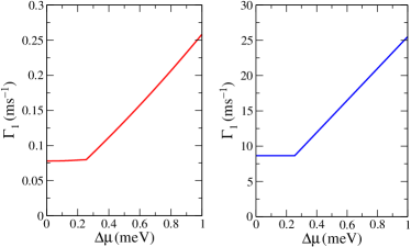
Figure 2: Relaxation rate $\Gamma_{1}=1/T_{1}$ as a function of the bias $\Delta\mu$ applied to the QPC for cases (ii) and (iii), see Sec. IV.A. The magnetic field ${{\bm{B}}}$ is along $x^{\prime}$ with magnitude $B=10$ T.

VI Concluding Remarks

In conclusion, we have shown that charge read-out devices (e.g. a QPC charge detector) induces spin decay in quantum dots due to the spin-orbit interaction (both Rashba and Dresselhaus). Due to the transverse nature of the fluctuating quantum field $\delta{{\bm{B}}}(t)$, we found that pure dephasing is absent and the spin decoherence time $T_{2}$ becomes twice the relaxation time $T_{1}$, i.e. $T_{2}=2T_{1}$. Finally, we showed that the spin decay rate is proportional to the shot noise of the QPC in the regime of large bias ($\Delta\mu\gg E_{Z}$) and scales as $a^{-6}$ (see Fig. 1). Moreover, we have shown that this rate can be minimized by tuning certain geometrical parameters of the setup. Our results should also be useful for designing experimental setups such that the spin decoherence can be made negligibly small while charge detection with the QPC is still efficient.

We thank J. Lehmann, W. A. Coish, T. Heikkilä, H. Gassmann and S. Erlingsson for helpful discussions. This work was supported by the Swiss NSF, the NCCR Nanoscience, EU RTN Spintronics, DARPA, and ONR.

Appendix A Schrieffer-Wolff transformation

To derive the expression for $S$, we note that applying $\frac{1}{L_{d}^{n}}$ on ${\bm{\xi}}$ yields linear combinations of momentum and position operators. Therefore we make an ansatz for $S$, like we did in Eq. (14), with

$$\mbox{\boldmath$\xi$}_{1} = \left((\alpha_{1}p_{y^{\prime}}+\alpha_{2}x^{\prime})/\lambda_{-},\,(\tilde{\alpha}_{1}p_{x^{\prime}}+\tilde{\alpha}_{2}y^{\prime})/\lambda_{+},\,0\right),\;\;\;\;\;\;\;$$ (75)

$$\mbox{\boldmath$\xi$}_{2} = \left((\beta_{1}p_{x^{\prime}}+\beta_{2}y^{\prime})/\lambda_{-},\,(\tilde{\beta}_{1}p_{y^{\prime}}+\tilde{\beta}_{2}x^{\prime})/\lambda_{+},\,0\right).\;\;\;\;\;\;\;$$ (76)

Then by inserting this ansatz into the relation $\left[H_{d}+H_{Z},S\right]=H_{SO}$, we obtain a set of algebraic equations for the coefficients $\alpha_{i}$, $\beta_{i}$, $\tilde{\alpha}_{i}$, and $\tilde{\beta}_{i}$ ($i=1,2$). We find that

$$\tilde{\alpha}_{1}=\alpha_{1},\;\;\;\;\;\;\;\;\tilde{\alpha}_{2}=-\alpha_{2},$$ (77)

$$\tilde{\beta}_{1}=-\beta_{1},\;\;\;\;\;\;\tilde{\beta}_{2}=\beta_{2},$$ (78)

with the coefficients $\alpha_{i}$ and $\beta_{i}$ given in Eqs. (17)-(20).

Appendix B $k$–dependent coupling constants, $k_{F}^{-1},\lambda_{\rm sc}\ll a$

The coupling constants ${\bm{\varepsilon}}_{ee}$, ${\bm{\varepsilon}}_{oo}$ and ${\bm{\varepsilon}}_{ee}$ are generally $k$-dependent. In the regime where $k_{F}^{-1},\lambda_{\rm sc}\ll a$ we obtain the following relations

$${\bm{\varepsilon}}_{ee} = \frac{e}{4\kappa a^{4}k^{3}}\{2k^{3}\lambda_{sc}(4a^{2}+3\lambda_{d}^{2}-2\lambda_{sc}^{2})+6k\lambda_{sc}\cos 2(k\lambda_{sc}+\delta)$$ (79)

$$-(3+4a^{2}k^{2}+3k^{2}\lambda_{d}^{2}-6k^{2}\lambda_{sc}^{2})\sin 2(k\lambda_{sc}+\delta)+(3+4a^{2}k^{2}+3k^{2}\lambda_{d}^{2})\sin(2\delta)\}\mbox{\boldmath${e}$}_{Y},$$

$${\bm{\varepsilon}}_{oo} = \frac{e}{4\kappa a^{4}k^{3}}\{2k^{3}\lambda_{sc}(4a^{2}+3\lambda_{d}^{2}-2\lambda_{sc}^{2})+6k\lambda_{sc}\cos(2k\lambda_{sc})-(3+4a^{2}k^{2}+3k^{2}\lambda_{d}^{2}-6k^{2}\lambda_{sc}^{2})\sin(2k\lambda_{sc})\}\mbox{\boldmath${e}$}_{Y},$$ (80)

$${\bm{\varepsilon}}_{oe} = \frac{e}{8\kappa a^{5}k^{4}}\{(9+4a^{2}k^{2}+3k^{2}\lambda_{d}^{2}-6k^{4}\lambda_{sc}^{4}+6k^{4}\lambda_{d}^{2}\lambda_{sc}^{2}+8a^{2}k^{4}\lambda_{sc}^{2})\cos\delta$$ (81)

$$-(9+4a^{2}k^{2}+3k^{2}\lambda_{d}^{2}-18k^{2}\lambda_{sc}^{2})\cos(2k\lambda_{sc}+\delta)-(9+4a^{2}k^{2}+3k^{2}\lambda_{d}^{2}-6k^{2}\lambda_{sc}^{2})2k\lambda_{sc}\sin(2k\lambda_{sc}+\delta)\}\mbox{\boldmath${e}$}_{X},\;\;\;\;\;\;\;\;\;\;$$

with $\delta$ being the relative scattering phase. The transformation to the Left-Right basis is given by

$${\bm{\varepsilon}}_{LL} = \frac{1}{2}({\bm{\varepsilon}}_{ee}+{\bm{\varepsilon}}_{oo}-2{\bm{\varepsilon}}_{eo}\cos\delta),$$ (82)

$${\bm{\varepsilon}}_{RR} = \frac{1}{2}({\bm{\varepsilon}}_{ee}+{\bm{\varepsilon}}_{oo}+2{\bm{\varepsilon}}_{eo}\cos\delta),$$ (83)

$${\bm{\varepsilon}}_{LR} = {\bm{\varepsilon}}_{RL}^{*}=\frac{1}{2}({\bm{\varepsilon}}_{ee}-{\bm{\varepsilon}}_{oo}+2i{\bm{\varepsilon}}_{eo}\sin\delta).\;\;\;\;\;\;$$ (84)

Here, as before, we have assumed that $\hbar v_{F}\Delta k\leq E_{Z}\ll\hbar v_{F}\lambda_{sc}^{-1}\ll E_{F}$. Note that the coupling constants ${\bm{\varepsilon}}_{LR}$ and ${\bm{\varepsilon}}_{RL}$ in Eq. (84) have both real and imaginary parts. Therefore, the last term in Eq. (60) does not vanish in general. Nevertheless, we find that for an in-plane magnetic field ${\bm{B}}=(B_{x},B_{y},0)$ this term vanishes, because only a single component of $\delta{\bm{B}}(t)$ (namely $\delta B_{z}(t)$, see Eq. (22)) is present for in-plane fields, which leads to $\epsilon_{kij}n_{k}{\cal J}^{-}_{ij}(\omega_{Z})=0$ (see also Eqs. (61) and (74)).

References

- (1) Semiconductor Spintronics and Quantum Computation, D.D. Awschalom, D. Loss, and N. Samarth (eds.), (Springer, Berlin, 2002).
- (2) S.A. Wolf, D. D. Awschalom, R. A. Buhrman, J. M. Daughton, S. von Molnár, M. L. Roukes, A. Y. Chtchelkanova, and D. M. Treger, Science 294, 1488 (2001).
- (3) I. Žutić, J. Fabian, and S. Das Sarma, Rev. Mod. Phys. 76, 323 (2004).
- (4) D. Loss and D.P. DiVincenzo, Phys. Rev. A 57, 120 (1998).
- (5) V. Cerletti, W. A. Coish, O. Gywat, and D. Loss, Nanotechnology 16, R27 (2005).
- (6) E. Buks, R. Schuster, M. Heiblum, D. Mahalu, and V. Umansky, Nature 391, 871 (1998).
- (7) S. Tarucha, D. G. Austing, T. Honda, R. J. van der Hage and L. P. Kouwenhoven, Phys. Rev. Lett. 77, 3613 (1996).
- (8) M. Ciorga, A.S. Sachrajda, P. Hawrylak, C. Gould, P. Zawadzki, S. Jullian, Y. Feng, and Z. Wasilewski, Phys. Rev. B 61, R16315 (2000).
- (9) J.M. Elzerman, R. Hanson, J. S. Greidanus, L. H. Willems van Beveren, S. De Franceschi, L. M. K. Vandersypen, S. Tarucha, and L. P. Kouwenhoven, Phys. Rev. B 67, 161308(R) (2003).
- (10) J.R. Petta, A.C. Johnson, C.M. Marcus, M.P. Hanson, and A.C. Gossard, Phys. Rev. Lett. 93, 186802 (2004).
- (11) R. Hanson, B. Witkamp, L. M. K. Vandersypen, L. H. Willems van Beveren, J. M. Elzerman, and L. P. Kouwenhoven, Phys. Rev. Lett. 91, 196802 (2003).
- (12) J.M. Elzerman, R. Hanson, L. H. Willems van Beveren, B. Witkamp, L. M. K. Vandersypen, and L. P. Kouwenhoven, Nature 430, 431 (2004).
- (13) R. Hanson, L. H. Willems van Beveren, I. T. Vink, J. M. Elzerman, W. J. M. Naber, F. H. L. Koppens, L. P. Kouwenhoven, and L. M. K. Vandersypen, Phys. Rev. Lett. 94, 196802 (2005).
- (14) M. Field, C.G. Smith, M. Pepper, D.A. Ritchie, J.E.F. Frost, G.A.C. Jones, and D.G. Hasko, Phys. Rev. Lett. 70, 1311 (1993).
- (15) Y. Levinson, Europhys. Lett. 39, 299 (1997).
- (16) I.L. Aleiner, N.S. Wingreen, and Y. Meir, Phys. Rev. Lett. 79, 3740 (1997).
- (17) H.-A. Engel, V. Golovach, D. Loss, L.M.K. Vandersypen, J.M. Elzerman, R. Hanson, L.P. Kouwenhoven Phys. Rev. Lett. 93, 106804 (2004)
- (18) V.N. Golovach, A. Khaetskii, and D. Loss, Phys. Rev. Lett. 93, 016601 (2004).
- (19) A.V. Khaetskii and Yu.V. Nazarov, Phys. Rev. B 64, 125316 (2001).
- (20) M. Kroutvar, Y. Ducommun, D. Heiss, M. Bichler, D. Schuh, G. Abstreiter, and J.J. Finley, Nature 432, 81 (2004).
- (21) G. Burkard, D. Loss, and D.P. DiVincenzo, Phys. Rev. B 59 2070 (1999).
- (22) A.V. Khaetskii, D. Loss, and L. Glazman, Phys. Rev. Lett. 88 186802 (2002); Phys. Rev. B 67 195329 (2003).
- (23) I.A. Merkulov, Al.L. Efros, and M. Rosen, Phys. Rev. B 65, 205309 (2002).
- (24) S.I. Erlingsson and Yu.V. Nazarov, Phys. Rev. B 66, 155327 (2002).
- (25) J. Schliemann, A.V. Khaetskii, and D. Loss, Phys. Rev. B 66, 245303 (2002).
- (26) R. de Sousa and S. Das Sarma, Phys. Rev. B 67, 033301 (2003).
- (27) W.A. Coish and D. Loss, Phys. Rev. B 70, 195340 (2004); W.A. Coish and D. Loss, Phys. Rev. B 72, 125337 (2005); D. Klauser, W.A. Coish, and D. Loss, cond-mat/0510177.
- (28) A.S. Bracker, E.A. Stinaff, D. Gammon, M.E. Ware, J.G. Tischler, A. Shabaev, Al.L. Efros, D. Park, D. Gershoni, V.L. Korenev, and I.A. Merkulov, Phys. Rev. Lett. 94, 047402 (2005).
- (29) F.H.L. Koppens, J.A. Folk, J.M. Elzerman, R. Hanson, L.H. Willems van Beveren, I.T. Vink, H.P. Tranitz, W. Wegscheider, L.P. Kouwenhoven, and L.M.K. Vandersypen, Science 309, 1346 (2005).
- (30) J.R. Petta, A.C. Johnson, J.M. Taylor, A. Yacoby, M.D. Lukin, C.M. Marcus, M.P. Hanson, and A.C. Gossard, Nature 435, 925 (2005).
- (31) J.R. Petta, A.C. Johnson, J.M. Taylor, E.A. Laird, A. Yacoby, M.D. Lukin, C.M. Marcus, M.P. Hanson, and A.C. Gossard, Science 309, 2180 (2005).
- (32) H.-A. Engel and D. Loss, Phys. Rev. lett. 86, 4648 (2001).
- (33) O. Gywat, H.-A. Engel, D. Loss, R.J. Epstein, F.M. Mendoza, and D.D. Awschalom, Phys. Rev. B 69, 205303 (2004).
- (34) O. Gywat, H.-A. Engel, and D. Loss, J. Supercond. 18, 175 (2005).
- (35) Y. Bychkov and E. I. Rashba, J. Phys. C 17, 6039 (1984).
- (36) G. Dresselhaus, Phys. Rev. 100, 580 (1955).
- (37) G. Mahan, Many Particle Physics, third edition (Plenum Press, New York, 2000).
- (38) S. Gustavsson, R. Leturcq, B. Simovic, R. Schleser, T. Ihn, P. Studerus, K. Ensslin, D. C. Driscoll, A.C. Gossard, cond-mat/0510269.
- (39) C.P. Slichter, Principles of Magnetic Resonance, (Springer-Verlag, Berlin, 1980).
- (40) D.P. DiVincenzo and D. Loss, Phys. Rev. B 71, 035318 (2005).
- (41) Ya.M. Blanter and M. Büttiker, Phys. Rep. 336, 1 (2000).