Computing Effective Hamiltonians of Doped and Frustrated Antiferromagnets By Contractor Renormalization

Abstract

A review of the Contractor Renormalization (CORE) method, as a systematic derivation of the low energy effective hamiltonian, is given, with emphasis on its differences and advantages over traditional perturbative (weak/strong links) real space RG. For the low energy physics of the 2D Hubbard model, we derive the plaquette bosons (projected SO(5)) model which connects the microscopic model to phases and phenomenology of high-T_c cuprates. For the S = 1/2 Pyrochlore and Kagomé antiferromagnets, the effective hamiltonians predict spin-disordered, lattice symmetry breaking, ground states with a large density of low energy singlets as found by exact diagonalization of small clusters.

I Relief From Strong Frustration

Frequently, interesting models of condensed matter systems involve strong local frustration. For example: the Heisenberg antiferromagnet given by

$$H=J\sum_{\langle ij\rangle}{\bf S}_{i}\cdot{\bf S}_{j},$$ (1)

where ${\langle ij\rangle}$ are nearest neighbor bonds on lattices depicted in Fig.1. The classical (infinite spin size) groundstates of the Pyrochlore and Kagomé lattices, are known to exhibit macroscopic (exponential in system size) degeneracy, which can be lifted by quantum fluctuations.

At low enough temperatures, one expects the third law of thermodynamics to ’kick in’ and that quantum fluctuations will choose a particular ground state. That ground state may, or may not, break spin rotational symmetry. However, sorting it out by semiclassical expansions such as spin wave theory, is a poorly controlled endeavor. In addition, numerical methods generally suffer from finite size limitations, and/or minus signs in quantum Monte Carlo simulations.

Frustration causes fierce competition between nearly degenerate variational states, and equally plausible mean field theories. Hence the phase diagram of such models are often a source of intense controversies. We advocate that such problems are best attacked by the ’divide and conquer’ approach within a systematic real-space renormalization scheme. The physical analogy is the use of nucleons, and then atoms, to treat the low energy correlations of the standard model. It is obvious, that questions in chemistry, such as the relative stability of molecules, are better resolved using effective interactions between atoms rather than by variational approximations on the high energy (’microscopic’) interactions.

Returning to condensed matter physics, we have adopted the approach invented by Morningstar and Weinstein called Contractor Renormalization (CORE)Morn96 to treat the square lattice Hubbard modelAltman02 , and several problems of frustrated quantum antiferromagnetsBerg03 ; Budnik04 . Other groups have also applied CORE to spin ladders PS97 , t-J laddersCap02 , and frustrated antiferromagnets Cap04 .

The essence of CORE is that the microscopic lattice Hamiltonian is mapped onto an effective Hamiltonian which acts on sites of a superlattice, within a lower energy Hilbert space, as we shall review below.

Figure 1: Strongly Frustrated Quantum Antiferromagnets treated by CORE. Red arrows denote classical spin directions. These can collectively rotate freely in the classical ground state manifold, rendering a poorly controlled spin wave expansion.

After an effective hamiltonian is found numerically, and represented in terms of familiar second quantized operators (bosons, fermions, pseudospins etc.) the remaining task is to determine its ground state and excitations. This could be carried out in different ways. If the effective model is still highly frustrated (as we shall find for the pyrochlore case), the CORE method could be reiterated. If the effective model turns out to be ’simple’, that is to say: apparently unfrustrated, it naturally lends itself to variational approaches, and quantum Monte-Carlo methods (as was done for the Projected SO(5) theory of the square lattice Hubbard modelpSO5 ; pSO5-num , and the Quantum Clock model of the Kagomé Budnik04 .)

We shall see that if the effective interactions produced by CORE were calculated to all ranges, upto the size of the full lattice, the resulting effective hamiltonian would reproduce the exact spectrum of the original Hamiltonian. However, this in itself does not yield saving of numerical effort. The success of CORE relies on a rapid decay of the effective interactions with range. This range, which is derived from the numerical convergence tests, describes the physical coherence length of the effective degrees of freedom used to describe thee effective hamiltonian: e.g. bosonic hole pairs, for the square lattice Hubbard model, or pseudospins for the local singlets of the pyrochlore model. Therefore, a proper choice of effective degrees of freedom is helpful for rapid convergence.

II CORE

CORE is a non-perturbative block-spin renormalization, which uses exact diagonalizations to extract the effective interactions.

1. Defining the reduced Hilbert Space. We first choose the elementary blocks which cover the lattice. (See Fig.2 for illustration for a square lattice). In order to preserve as much as possible the lattice symmetries of the original model (a choice of covering always breaks some translational symmetry), an optimal choice would be blocks which have the original rotational symmetries: such as plaquettes in a square lattice, triangles in the Kagomé and triangular lattices, and teterahedra in the pyrochlore lattice.

   We diagonalize ${\cal H}$ on a single block and truncate all states above a chosen cutoff energy. This leaves us with the lowest $M$ states $\{{\,|\,{\alpha}\,\rangle\,}\}_{1}^{M}$. The reduced lattice Hilbert space is spanned by tensor products of retained block states ${\,|\,{\alpha}_{1},\ldots,{\alpha}_{N}\,\rangle\,}$. A case in point is the Hubbard model spectrum on a plaquette, which for the half filled case has 70 states (see Fig.4). We truncate 66 states and keep the ground state and lowest triplet, i.e. $M=4$. Thus, the Hilbert space is considerably reduced at the first step. The retained states are in essence the ’atoms’ of the new effective Hamiltonian. The next task is to find their effective mass and interactions by calculating the intersite interactions.

   

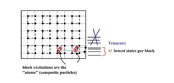
   Figure 2: Covering the square lattice with plaquettes as elementary blocks. The reduced Hilbert space is defined as the tensor products of the lowest $M$ states in each block.

2. The Renormalized Hamiltonian of any cluster. The reduced Hilbert space on a given connected cluster of $N$ blocks is of dimension ${\cal M}=M^{N}$. (See Fig. 3 for an illustration for N=3). We diagonalize ${\cal H}$ on the cluster and obtain the lowest ${\cal M}$ eigenstates and energies: $({\,|\,n\,\rangle\,},{\epsilon}_{n})$, $n=1,\ldots,{\cal M}$. The wavefunctions ${\,|\,n\,\rangle\,}$ are projected on the reduced Hilbert space and their components in the block basis ${\,|\,{\alpha}_{1},\ldots,{\alpha}_{N}\,\rangle\,}$ are obtained. The projected states $\psi_{n}$ are then Gramm-Schmidt orthonormalized, starting from the ground state upward.

   $${\,|\,\tilde{\psi}_{n}\,\rangle\,}={1\over{Z_{n}}}\left({\,|\,\psi_{n}\,\rangle\,}-\sum_{m<n}{\,|\,\tilde{\psi}_{m}\,\rangle\,}{\,\langle\,\tilde{\psi}_{m}\,|\,\psi_{n}\,\rangle\,}\right),$$ (2)

   where $Z_{n}$ is the normalization. The renormalized Hamiltonian is defined as

   $${\cal H}^{ren}\equiv\sum_{n}^{{\cal M}}{\epsilon}_{n}{\,|\,\tilde{\psi}_{n}\,\rangle\,}{\,\langle\,\tilde{\psi}_{n}\,|\,},$$ (3)

   which ensures that it reproduces the lowest ${\cal M}$ eigenenergies exactly.

   

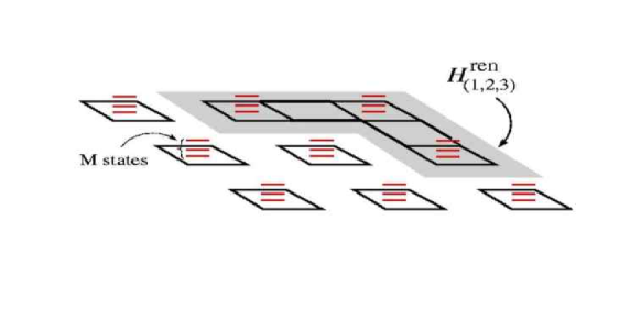
   Figure 3: A Cluster of 3 blocks, defining the effective Hamiltonian ${\cal H}^{ren}$ of range 3.

   Representing ${\cal H}^{ren}$ in the real space block basis ${\,|\,{\alpha}_{1},\ldots,{\alpha}_{N}\,\rangle\,}$, defines the (reducible) inter-block couplings and interactions.

3. Cluster expansion. We define connected $N$ point interactions as:

   $$h_{i_{1},\ldots,i_{N}}=H^{ren}_{\langle{i_{1},\ldots,i_{N}\rangle}}-\sum_{\langle{i_{1},\ldots,i_{N}^{\prime}\rangle}}h_{i_{1},\ldots,i_{N}^{\prime}},$$ (4)

   where the sum is over connected subclusters of $\langle i_{1},\ldots,i_{N}\rangle$. The full lattice effective Hamiltonian can be expanded as the sum

   $${\cal H}_{eff}=\sum_{i}h_{i}+\sum_{\langle ij\rangle}h_{ij}+\sum_{\langle ijk\rangle}h_{ijk}+...$$ (5)

   $h_{i}$ is simply a reduced single block hamiltonian. $h_{ij}$ contains nearest neighbor couplings and corrections to the on-site terms $h_{i}$. $h_{ijk}$ contains three site couplings and so on. $h_{i_{1},\ldots,i_{N}}$ will henceforth be called range-N interaction. We expect on physical grounds that for a proper choice of a truncated basis, range-N interactions will decay rapidly with $N$. This expectation needs to be verified on a case by case basis.

In general, there is no a priori quantitative estimation of the truncation error. Nevertheless, if it decays rapidly with interaction range, we deduce that there is a short coherence length related to our local degrees of freedom, e.g. in our case the hole pair bosons and the triplets (bound states of two spinons).

II.1 Comparison to perturbative real-space RG

Perturbative real-space Renormalization of Quantum Many-Body systems is carried out in either the Lagrangian or Hamiltonian formulation. The Lagrangian renormlization involves integrating out of the path integral high wavevector and frequency modes $\psi_{\rm high}$. For example, in a model with point interactions of strength $g$, the renormalization is carried out by expanding the exponential in powers of $g$: models

$$L^{\rm pert}[\psi_{\rm low}] = -\ln{1\over Z}\int{\cal D}\psi_{\rm high}\exp\left(-\psi^{*}L^{(2)}\psi-g|\psi|^{2}\right)$$ (6)

$$\approx \psi^{*}(x,\tau)\left(L^{(2)}+\Sigma(\tau-\tau^{\prime})\right)\psi(x^{\prime},\tau^{\prime})+g^{\rm ren}|\psi|^{2}+{\cal O}(g^{4})$$

This formulation always truncates higher order terms in $g$ (loops). It also necessarily introduces time-retarded interactions. This procedure usually results in a Lagrangian which similar to the microscopic one but with renormalized coupling constants. This allows an iterative renormalization (the renormalization group). However time retardation, if not neglected, divorces the Lagrangian formulation from the operator Hamiltonian formulation.

The alternative is a perturbative Hamiltonian renormalization scheme. However, the traditional (non CORE) approach does not avoid the limitations of perturbation theory and time retardation. First one the Hamiltonian is separated into block terms ($H_{0}$) and inter-block interactions ($H^{\prime}$).

$$H=H_{0}+H^{\prime}$$ (7)

The second step is to write the effective two-site hamiltonian in terms of a Brillouin-Wigner (BW) perturbation theory in the same reduced Hilbert space as CORE given by by the tensor products of the truncated block states $|\alpha_{i}\rangle$.

$${\cal H}^{\rm BW}=H_{0}+H^{\prime}+H^{\prime}\sum_{n=1}^{\infty}\left({1-P_{0}\over E-H_{0}}H^{\prime}\right)^{n}$$ (8)

where

$$P_{0}=\prod_{i}\sum_{\alpha_{i}=1}^{\cal M}|\alpha_{i}\rangle\langle\alpha_{i}|.$$ (9)

The expansion for ${\cal H}^{\rm BW}$ contains intercluster interactions of all ranges, and the sizes of the terms is controlled by $H^{\prime}/\Delta$ where $\Delta$ is a typical gap energy in the spectrum of $H_{0}$. The appearance of $E$ inside ${\cal H}^{\rm BW}(E)$ is a signature of time retarded interactions. It means that the spectrum is not given by the eigenvalues of ${\cal H}^{\rm BW}(E_{0})$ for any choice of $E_{0}$!

In summary, CORE has two major advantages over traditional perturbative real-space renormalization schemes:

1. CORE is not an expansion in weak/strong bonds between block-spins. Its convergence does not necessarily depend on existence of a large gap to the discarded states of the Hilbert space.

2. CORE is based on an exact mapping from the original Hamiltonian to an effective Hamiltonian, whose truncation error can be estimated numerically. Non-Hamiltonian retardation effects are avoided.

III Square lattice Hubbard Model

An important interacting many-body model, especially in the context of high temperature superconductors, is the square lattice Hubbard model given by

$${\cal H}=-t\sum_{\langle ij\rangle,s}^{sl}\left(c^{\dagger}_{is}c^{{}^{\vphantom{\dagger}}}_{js}+\mbox{H.c}\right)+U\sum_{i}n_{i\uparrow}n_{i\downarrow},$$ (10)

where $c^{\dagger}_{is},n_{is}$ are electron creation and number operators at site $i$ on the square lattice. Following the CORE procedure we choose to cover the square lattice by plaquettes (as in Fig.2). The low spectrum of 2, 3, and 4 electrons (2, 1 and no holes respectively) is depicted in Fig.4.

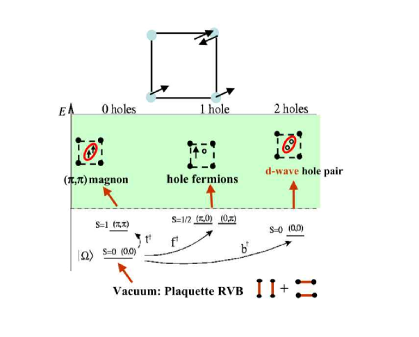
Figure 4: The low spectrum of the four site Hubbard model. Eigenstates are labeled by total spin $S$ and plaquette momentum $Q_{x},Q_{y}=0,\pi$. The undoped ground state is the vacuum, and the excitations are labeled by boson and fermion operators acting on that vacuum.

The ground state of the 4-site Hubbard model at half filling ($n_{e}=4$) is called ${\,|\,{\Omega}\,\rangle\,}$. which corresponds at large $U/t$ to the resonating valence bonds (RVB) ground state of the Heisenberg model plus small contributions from doubly occupied sites. The product state ${\,|\,{\Omega}\,\rangle\,}=\prod_{i}^{plaq}{\,|\,{\Omega}\,\rangle\,}_{i}$, is our vacuum state for the full lattice, upon which Fock states can be constructed using second quantized boson and fermion creation operators.

The magnons are defined by the undoped plaquettes which are in the lowest triplet of $S=1$ states.

The hole pair state at ($n_{e}=2$) is described by

$$b^{\dagger}_{\alpha}{\,|\,{\Omega}\,\rangle\,} = {1\over\sqrt{Z_{b}}}{\cal P}c^{\dagger}_{(0,0)\uparrow}c^{\dagger}_{(0,0)\downarrow}|0\rangle$$ (11)

$$= {1\over\sqrt{Z^{\prime}_{b}}}\left(\sum_{ij}d_{ij}c_{i\uparrow}c_{j\downarrow}+\ldots\right){\,|\,{\Omega}\,\rangle\,},$$

where $d_{ij}$ is +1 (-1) on vertical (horizontal) bonds, and $\ldots$ are higher order $U/t$-dependent operators. Thus, $b^{\dagger}$ creates a pair with internal $d$-wave symmetry with respect to the vacuum. For the relevant range of $U/t$, the state normalization is $1/3<Z_{b}^{\prime}<2/3$. The important energy to note is the pair binding energy defined as

$${\Delta}_{b}\equiv E(0)+E(2)-2E(1)$$ (12)

where $E(N_{h})$ is the ground state of $N_{h}$ holes. In the range $U/t\in(0,5)$, it is bounded by $-0.04t<{\Delta}_{b}<0$. It has been well appreciated that the Hubbard, t-J and even CuO₂ models have pair binding in finite clusters starting with one plaquette.

A d-wave superconducting state can be written as the coherent state

$$\Psi^{d-scF}\equiv\prod_{i}^{plaq}(\cos\theta+\sin\theta e^{i\varphi}b^{\dagger}_{i}){\,|\,{\Omega}\,\rangle\,},$$ (13)

with the superconductor order parameter

$$\langle\Psi|d_{ij}c_{i\uparrow}c_{j\downarrow}|\Psi\rangle=\sqrt{Z_{b}^{\prime}}e^{i\varphi}\sin\theta\cos\theta.$$ (14)

Both the triplets and the hole pairs are ’bosonic states’, which can be represented by boson creation operators acting on the RVB vacuum. They do not carry a negative sign under exchange.

The single hole (3 electrons) ground states are fermions. Since they are slightly higher in energy than the hole pair states, we truncate the spectrum below them (at our peril, of course!), for the sake of deriving a purely bosonic effective hamiltonian, with hopefully rapidly decreasing interactions at long range.

III.1 The Plaquette-Boson, (Projected SO(5)) Model

We present the CORE calculations to range-2 boson interactions, while projecting out the fermion states. This required a modest numerical diagonalization effort of the Hubbard model on up to 8 site clusters. The resulting range-2 Plaquette Boson (PB) model can be separated into bilinear and quartic (interaction) terms:

$${\cal H}^{\rm pb}={\cal H}^{b}[b]+{\cal H}^{t}[t]+{\cal H}^{int}[b,t]$$ (15)

where the bosons obey local hard core constraints

$$b^{\dagger}_{i}b_{i}+\sum_{\alpha}t^{\dagger}_{\alpha i}t_{\alpha i}\leq 1$$ (16)

The bilinear energy terms are

$${\cal H}^{\rm b} = (\epsilon_{b}-2\mu)\sum_{i}b^{\dagger}_{i}b^{{}^{\vphantom{\dagger}}}_{i}-J_{b}\sum_{\langle ij\rangle}\left(b^{\dagger}_{i}b^{{}^{\vphantom{\dagger}}}_{j}+\mbox{H.c.}\right)$$

$${\cal H}^{t} = \epsilon_{t}\sum_{i\alpha}t^{\dagger}_{\alpha i}t^{{}^{\vphantom{\dagger}}}_{\alpha i}-{J_{t}\over 2}\sum_{\alpha\langle ij\rangle}(t^{\dagger}_{\alpha i}t^{{}^{\vphantom{\dagger}}}_{\alpha j}+\mbox{H.c.})$$ (17)

$$~{}~{}-{J_{tt}\over 2}\sum_{\alpha\langle ij\rangle}(t^{\dagger}_{\alpha i}t^{\dagger}_{\alpha j}+\mbox{H.c.}).$$

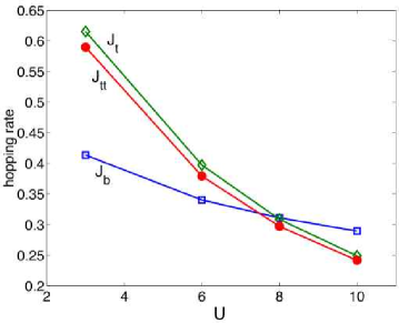
Figure 5: CORE results for the effective boson hopping rates corresponding to Hubbard interaction $U$ (in units of $t$). $J_{b}$ is the $d$-wave hole pair hopping rate, and $J_{t}$ and $J_{tt}$ are magnetic energy scales defined in (17). Note near equality of hopping energies around $U/t=8$, signaling the projected SO(5) point.

In Fig. 5 we compare the magnitudes of the magnon hoppings $J_{t},J_{tt}$ and the hole pair hopping $J_{b}$ for a range of $U/t$. The region of intersection near $U/t=8$, is close to the projected SO(5) symmetry point. We emphasize that although there is no quantum SO(5) symmetry in $H^{\rm pb}$, there is an approximate equality of the bosons hopping energy scales. This equality which was assumed in the pSO(5) theorypSO5 , previously appealed to phenomenological considerations. Here, the equality emerges in a physically interesting regime of the Hubbard model and has important consequences on the phase diagram as was shown in Ref.pSO5-num .

III.2 CORE convergence and Coherence Length

By diagonalizing the 12 site clusters, we have found that range 3 interactions are indeed between 1-10% of the range 2 interactions. Computing range 3 interactions $h_{123}$ and finding out whether they are significantly smaller than range 2 terms is important for two main reasons: (i) This is the only way one could validate a truncation of the cluster expansion to range 2 for further investigations of the low energy properties of the model, and (ii) a rapid decrease in effective interactions signals a short ’coherence lengthscale’ which describes the size of the effective degrees of freedom. For cuprates, the effective size of the hole pair is of experimental importance, since it is bounded by the superconducting coherence length as observed by the vortex core size, and the short superconducting healing length near grain boundaries and defects. Both have been observed to be not much larger than a few lattice constants.

IV Pyrochlores

The pyrochlore lattice is depicted in Fig.1. Depicted in Fig. 6 is the spectrum of the Quantum Heisenberg model (1) on a 4-site tetrahedron and a 16 site supertetrahedron. Both blocks can be used to cover the Pyrochlore lattice. Their block ground states are doubly degenerate singlets, and thus the effective hamiltonians are readily described by pseudospin-half operators.

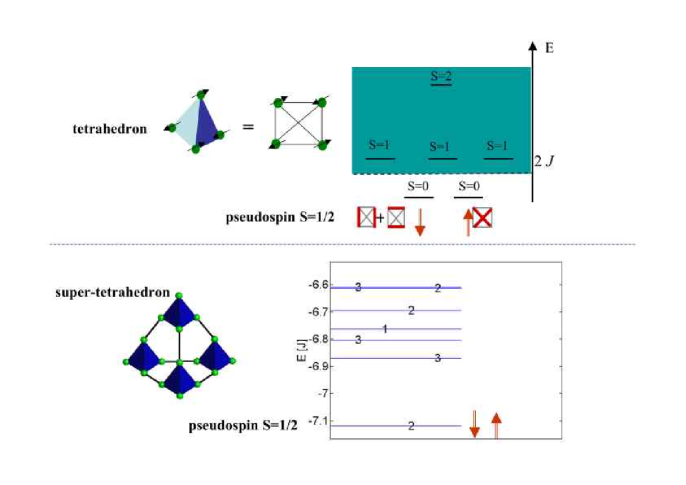
Figure 6: The low spectrum of the Heisenberg model on a tetrahedron, and a supertetrahedron. In both clusters the ground states are degenerate singlets which can be represented by spin half eigenstates.

Using CORE for the tetrahedra covering upto range 3, we have found

$$H^{\rm FCC} =\sum_{\langle ijk\rangle}\Bigg{(}(J_{2}({\bf S}_{i}\cdot{\bf e}^{(i)}_{ijk})({\bf S}_{j}\cdot{\bf e}^{(j)}_{ijk})-$$

$$J_{3}(\frac{1}{2}-{\bf S}_{i}\cdot{\bf e}^{(i)}_{ijk})(\frac{1}{2}-{\bf S}_{j}\cdot{\bf e}^{(j)}_{ijk})(\frac{1}{2}-{\bf S}_{k}\cdot{\bf e}^{(k)}_{ijk})\Bigg{)}.$$

The coupling parameters (in units of $J$) are: $J_{2}=0.1049$, $J_{3}=0.4215$, and ${\bf e}^{(i)}_{123},i=1,2,3$ are three unit vectors in the x-y plane whose angles ${\alpha}^{(i)}_{123}$ depend on the particular plane defined by the triangle of tetrahedral units $123$ as given in table I of ts02 . The effective hamiltonian (IV) resembles the terms obtained by Tsunetsugu by second order perturbation theory (in inter-tetrahedra couplings) ts02 . The classical mean field ground state is three of the four FCC sublattices are ordered in the directions ${\bf e}(0),{\bf e}(2\pi/3),{\bf e}(-2\pi/3)$, while the direction of the fourth is completely degenerate. Therefore, classical mean field approximation for (IV) is insufficient to remove the ground state degeneracy. Tsunetsuguts02 was able to lift the degeneracy by including spinwave fluctuations effects which produce ordering at a new low energy scale.

Here we avoid the a-priori symmetry breaking needed for semiclassical spinwave theory, by treating (IV) fully quantum mechanically. This entails a second CORE transformation which involves choosing the “supertetrahedron”, as a basic cluster of four tetrahedra.

Our new pseudospins ${\bf\tau}_{i}$ are defined by the two degenerate singlet ground states of the supertetrahedron. (This degeneracy is found for the Heisenberg model on the original lattice as well as for the effective model (IV)). These states transform as the E irreducible representation of the tetrahedron ($T_{d}$) symmetry group, similarly to the singlet ground states of a single tetrahedron.

The supertetrahedra form a cubic lattice. The effective hamiltonian (IV) and the lattice geometry imply that non-trivial effective interactions appear only at the range of three supertetrahedra and higher. Range three effective interactions include two and three pseudospin interactions, which are dominated by

$$\mathcal{H}^{\rm Cubic} = J_{1}\sum_{\langle ij\rangle}{({\bf\tau}_{i}\cdot{\bf f}_{ij})({\bf\tau}_{j}\cdot{\bf f}_{ij})}+$$

$$J^{(a)}_{2}\sum_{\langle\langle ij\rangle\rangle}{({\bf\tau}_{i}\cdot{\bf f}_{ij})({\bf\tau}_{j}\cdot{\bf f}_{ij})}+$$

$$J^{(b)}_{2}\sum_{\langle\langle ij\rangle\rangle}{({\bf\tau}_{i}\cdot({\bf f}_{ij}\times\hat{\bf z}))({\bf\tau}_{j}\cdot({\bf f}_{ij}\times\hat{\bf z})}).$$

Here, $\langle~{}\rangle$ and $\langle\langle~{}\rangle\rangle$ indicate summation over nearest- and next nearest-neighbors, respectively. The coupling constants are found to be relatively small: $J_{1}=0.048J$, $J^{(a)}_{2}=-0.006J$ and $J^{(b)}_{2}=0.018J$ . The vectors ${\bf f}_{ij}$ depend on the vector ${\bf r}_{ij}$ connecting the two sites, and their values are presented in Ref.Berg03 .

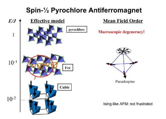
Figure 7: Two CORE steps to relieve frustration in the Pyrochlore model. The first step results in an FCC pseudospin model whose mean field solution has one sublattice of completely free spins. The second CORE step results in a simple cubic model, with renormalized coupling constant of $\sim 0.01J$, which has no residual macroscopic degeneracy. Its pseudospins, (which are represented by singlets on 16-site super-tetrahedra), are antiferromagnetically correlated between neighboring planes.

We performed classical Monte Carlo simulations using the classical (large spin) approximation to (IV). The ground state was found to choose an antiferromagnetic axis, and to be ferromagnetic in the planes as depicted in Fig. 7. It differs from the semiclassical ground statets02 . The latter involves condensation of high energy states of the supertetrahedron in the thermodynamic ground state. Since on a supertetrahedra we find a much larger gap to these states than inter-site coupling, we believe they cannot condense to yield the semiclassical ground state symmetry breaking.

To estimate the truncation error we calculated the contribution of range-4 interactions in both stages of CORE leading to (IV) and (IV). Evidently, these terms are small ($<30\%$), and most importantly, including them does not alter the mean field solution.

V The Kagomé

The Heisenberg model (1) on the Kagomé lattice (depicted in Fig.1) has macroscopic degeneracy in its classical ground state. For the initial stage of CORE, we choose the upward triangles covering, and a truncated basis of the four degenerate spin half ground states, discarding the higher $S=3/2$ states, see Fig.8.,

Figure 8: CORE on the Kagomé. Up-triangles provide four degenerate groundstates, which can represent a spin and a pseudospin of sizes half on each block.

The S-L representation of the four ground states are labeled by $|s,l\rangle$, where $s=\uparrow,\downarrow$ is the magnetization and $l=\Uparrow,\Downarrow$ is the pseudospin in the $z$ direction. Explicitly, in the Ising basis $|s_{1}s_{2}s_{3}\rangle$,

$$|s,\Uparrow\rangle = {(|s\uparrow\downarrow\rangle-|s\downarrow\uparrow\rangle)\over\sqrt{2}}$$

$$|s,\Downarrow\rangle = {|s\uparrow\downarrow\rangle+|s\downarrow\uparrow\rangle)\over\sqrt{6}}-\sqrt{2\over 3}|(-s)ss\rangle$$ (20)

The pseudospin direction in the $xz$ plane correlates with the direction of the singlet bond, e.g. $\Uparrow$ describes a singlet dimer on the bottom ($-\hat{z}$) edge. Thus, the $L^{y}$ eigenstates have definite chiralities.

V.1 The SL Hamiltonian

. The effective interactions between triangles is calculated by CORE. We note that this approach is feasible when two conditions are met: (i) Interaction matrix elements fall off rapidly with range such that the truncation error at finite ranges is small, and (ii) the norms of the projected eigenstates are sufficiently large for numerical accuracy. We have computed all range 2 and range 3 interactions, and neglected range 4 corrections, whose expectation values were found to be an order of magnitude smaller. At range 3, norms of projected eigenstates were greater than 0.75, with most states above 0.9.

The effective Hamiltonian is a Spin-Pseudospin (SL) Model on the triangular lattice:

$${\cal H}_{SL} = {\cal H}_{ss}+{\cal H}_{ll}$$

$${\cal H}_{ss} = \sum_{\langle ij\rangle}{\bf S}_{i}\cdot{\bf S}_{j}~{}\left[J_{ss}+J_{sslele}({\bf L}_{i}\cdot{\bf e}_{ij})\cdot({\bf L}_{j}\cdot{\bf e}_{ji})\right.$$

$$+J_{ssll}({\bf L}^{\perp}_{i}\cdot{\bf L}^{\perp}_{j})+J_{ssle1}({\bf L}_{i}\cdot{\bf e}_{ij})$$

$$\left.+J_{ssle2}({\bf L}_{j}\cdot{\bf e}_{ji})+J_{sslyly}{\bf L}_{i}^{y}{\bf L}_{j}^{y}\right]$$

$${\cal H}_{ll} = J_{lele}({\bf L}_{i}\cdot{\bf\tilde{e}}^{ij})\cdot({\bf L}_{j}\cdot{\bf\tilde{e}}_{ji})+J_{ll}({\bf L}^{\perp}_{i}\cdot{\bf L}^{\perp}_{j})$$ (21)

$$+J_{lyly}{\bf L}_{i}^{y}{\bf L}_{j}^{y}$$

Here ${\bf L}^{\perp}=({\bf L}^{x},{\bf L}^{z})$, and ${\bf e}_{ij},{\bf e}_{ij}^{l}$ are unit vectors in the $xz$ plane. ${\cal H}_{ss}$ describes interactions of the Kugel-Khomskii type, where the pseudospin exchange anisotropy depends on the sites and bond directions. For any other other bond $\langle ij^{\prime}\rangle$, ${\bf e}_{ij^{\prime}}$ is simply found by rotating ${\bf e}_{ij}$ by $0,\pm 120^{\circ}$ according to the O(2) rotation of $\langle ij\rangle\to\langle ij^{\prime}\rangle$.

V.2 Ground state and Low Excitations

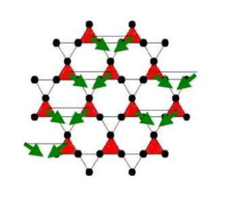
Figure 9: Variational minimum of the SL Hamiltonian. Arrows denote pseudospin directions, and solid lines denote singlet spin correlations between neighboring blocks. The ground state is a columnar dimer state of neighboring up-triangle singlets.

The best variational candidate for the SL model (21) are the dimer coverings of two triangle singlets, whose correlations are defined by Fig. 9. The dimer singlet states have been shown by Mila and MambriniMM to span much of the low singlet spectrum in finite cluster calculations. The variational analysis highlights the special role of the “Dimerization Fields”, $J_{ssle_{1}},J_{ssle_{1}}$ in (21), for the formation of local singlets. These terms cancel under summation in all uniform states defined by $\langle{\bf S}_{i}{\bf S}_{j}\rangle=\mbox{const}$. Their significant magnitude helps to lower the energy considerably by aligning ${\bf L}_{i}$ with the anisotropy vectors ${\bf e}_{ij}$ to form singlets on certain bonds and not on others $\langle{\bf S}_{i}\cdot{\bf S}_{j}\rangle=-{3\over 4}\delta_{\langle ij\rangle_{dim}}$. This is a strong argument in favor of a paramagnetic ground state. Consequently, ${\cal H}_{ll}$ is crucial in selecting the true ground state among the multitude of dimer singlet coverings. We have found that the perfectly ordered columnar dimer (CD) state minimizes ${\cal H}_{ll}$. A local “defect” of a rotated dimer in the CD background costs a “twist” energy of $+0.01$ per site. In (Budnik04 ) a theory of long wavelength fluctuations about the CD state has been investigated. The theory has a 6-fold ’clock mass term’ $u_{6}\cos(6\phi)$, which yields a finite gap. However, quantum fluctuations renormalize down the magnitude of the clock mass to exponentially low values due to the 6 fold symmetry. This may explain the large density of low energy singlet excitations observed numericallysinglets , and predicts a $T^{2}$ temperature dependence of the specific heat due to singlet excitations.

VI Summary

In summary I have reviewed our group’s recent applications of CORE to currently interesting problems of strong quantum frustration, e.g.: the 2D Hubbard model for cuprates, and the geometrically frustrated Heisenberg model. We find that the effective Hamiltonians are not necessarily simpler in form, but in a many cases they reveal the low energy degrees of freedom as the eigenstates of small clusters. The effective interactions, if they decay rapidly in space, may yield less competition and frustration than in the microscopic Hamiltonian, and thus be better amenable to variational solutions.

In the computational sense, one could view CORE as an efficient algorithm to obtain the low energy physics of a large many body system, which maximally extracts its information from exact diagonalizations of small clusters. In combination with other approaches, this provides a promising direction to disentangle the low energy physics of strongly correlated many body problems. The method allows self-estimation of convergence, by sampling interactions of higher ranges than are retained.

VI.1 Acknowledgments

I thank my collaborators E. Altman, E. Berg and R. Budnik, and acknowledge fruitful discussions with S. Capponi, D. Poilblanc and R. Moessner. I acknowledge grants from US-Israel Binational Science Foundation and the Israel Science Foundation.

References

- (1) C. Morningstar and M. Weinstein, Phys. Rev. D 54, 4131 (1996).
- (2) E. Altman and A. Auerbach, Phys. Rev. B 65, 104508 (2002).
- (3) E. Berg, E. Altman and A. Auerbach, Phys. Rev. Lett. 90, 147204 (2003).
- (4) R. Budnik and A. Auerbach, Phys. Rev. Lett. 93, 187205 (2004).
- (5) S. Piekarewicz and J.R. Shepard, Phys. Rev. B56, 5366 (1997).
- (6) S. Capponi and D. Poilblanc, Phys. Rev. B66, 180503 (2002).
- (7) S. Capponi, A. Lauchli and M. Mambrini, Phys. Rev. B 70, 104424 (2004).
- (8) S-C. Zhang, J-P. Hu, E. Arrigoni, W. Hanke and A. Auerbach, Phys. Rev. B60, 13060 (1999).
- (9) A. Dorneich, W. Hanke, E. Arrigoni, M. Troyer, and S. C. Zhang, Phys. Rev. Lett. 88, 057003 (2002).
- (10) H. Tsunetsugu, Phys. Rev. B 65, 024415 (2002).
- (11) F. Mila, Phys. Rev. Lett. 81, 2356 (1998); M. Mambrini and F. Mila, Eur. Phys. J. B 17 651 (2000).
- (12) P. Lecheminant, B. Bernu, C. Lhuillier, L. Pierre and P. Sindzingre, Phys. Rev. B 56, 2521 (1997); C. Waldtmann, H.-U. Everts, B. Bernu, C. Lhullier, P. Sindzingre, P. Lecheminant and L. Pierre, Eur. Phys. J. B 2 501 (1998).