Transport in polymer-gel composites: Response to a bulk concentration gradient

Abstract

This paper examines the response of electrolyte-saturated polymer gels, embedded with charged spherical inclusions, to a weak gradient of electrolyte concentration. These composites present a model system to study microscale electrokinetic transport processes, and a rigorous theoretical prediction of the bulk properties will benefit novel diagnostic applications. An electrokinetic model was presented in an earlier publication, and the response of homogeneous composites to a weak electric field was calculated. In this work, the influence of the inclusions on bulk ion fluxes and the strength of an electric field (or membrane diffusion potential) induced by the bulk electrolyte concentration gradient are computed. Effective ion diffusion coefficients are significantly altered by the inclusions, so—depending on the inclusion surface charge or $\zeta$-potential—asymmetric electrolytes can behave as symmetrical electrolytes, and vice versa. The theory also quantifies the strength of flow driven by concentration-gradient-induced perturbations to the equilibrium diffuse double layers. Similarly to diffusiophoresis, the flow may be either up or down the applied concentration gradient.

I Introduction

Permeable membranes are the basis of molecular separation and sorting technologies, including ion exchange, gel-electrophoresis chromatography, and dialysis (Lakshminarayanaiah:1969, ). Ion permeable membranes are also vital to batteries, fuel cells, electrochemical sensors, and biological cells (Sten-Knudsen:2002, ). In this work, a theoretical model of electrolyte transport in membranes comprised of a continuous polymer gel with charged spherical inclusions is used to investigate the influence of the inclusions on bulk ion fluxes. Because several important characteristics of the microstructure can, in principle, be carefully controlled, these materials present a model system for studying fundamental aspects of electrokinetic transport processes. An ability to tailor the microstructure and accurately predict the bulk properties could also make these materials useful in novel diagnostic applications (e.g., Hagedorn:2005, ).

Electrolyte diffusion in the absence of electromigration is accompanied by a net flux of charge when anion and cation mobilities are not equal. Therefore, an electric field is necessary to compensate for the net diffusive flux of charge across a membrane. In biological cells, ion mobilities are regulated by transmembrane proteins (ion channels), and electrical signaling is achieved by controlling the relative ion mobilities (Sten-Knudsen:2002, ). In diagnostic electrochemical cells, diffusion potentials are deleterious, and their influence is usually attenuated by a salt bridge containing a concentrated symmetrical electrolyte (e.g., KCl). When charged inclusions are immobilized in an electrically neutral polymer gel, the effective ion mobilities are altered, so even symmetrical electrolytes my behave as highly asymmetric electrolytes; this paper provides a first step toward quantifying this influence.

When aqueous NaCl, for example, is brought into contact with negatively charged inclusions (e.g., silica), the counter-ion (Na⁺) is concentrated in the diffuse double layers. A gradient of electrolyte concentration perturbs the equilibrium state, inducing diffusion and electromigration to restore local equilibrium. At the surfaces of inclusions facing up the concentration gradient, the equilibrium gradient of electrostatic potential attracts counter-ions and repels co-ions, leading to inner and outer layers of perturbed charge density. The accompanying electric field acts on the underlying equilibrium charge, driving layers of backward and forward electroosmotic flow. In this work, non-linear perturbations are neglected because the perturbing ‘forces’ are weak compared to those of the underlying equilibrium state. Accordingly, the theory is limited to weak electrolyte concentration gradients.

Perturbations enhance the net flux of counter-ions (Na⁺), because counter-ions are accumulated (depleted) at the surfaces facing up (down) the bulk concentration gradient. The resulting (tangential) concentration gradient increases the net (diffusive) counter-ion flux. Note that the accompanying perturbed charge density produces an electric field that induces an electromigrative flux of counter-ions down the bulk concentration gradient. Therefore, because Na⁺ ions have a lower mobility than Cl^-, both contributions to the net flux counteract the tendency of Na⁺ to otherwise diffuse more slowly than Cl^-. Overall, negatively charged inclusions increase the (effective) symmetry of the electrolyte. Since the degree of electrolyte symmetry bears directly on the membrane diffusion potential, the diffusion potential characterizes the physicochemical state of the inclusion-electrolyte interface.

The theoretical model adopted in this work was developed and applied in an earlier publication to examine ion fluxes and electroosmotic flow driven by an applied electric field (Hill:2005b, ). In homogeneous membranes, diffusive and electromigrative transport are significantly influenced by the charge of the inclusions, but not by the hydrodynamic permeability of the polymer gel. On the other hand, electroosmotic flow is very sensitive to the gel permeability and reorganization of charge by diffusion and electromigration. These characteristics are expected to prevail with the application of a bulk concentration gradient, as examined in this paper.

Note that there is a close connection of this work to earlier studies of diffusiophoresis (Prieve:1984, ; Prieve:1987, ; Anderson:1989, ), which address the motion of colloidal particles induced by solute concentration gradients. Fluid motion induced by solute concentration gradients at stationary charged interfaces is referred to as diffusioosmosis (Dukhin:1974, ), and this, perhaps, best characterizes the phenomena investigated here. Note that Wei and Keh (Wei:2003, ) derived semi-analytical predictions of the flow induced by solute concentration gradients in (ordered) fibrous porous media. Their calculations are restricted to low surface potentials, however, and their theory adopts a so-called cell model to handle fiber-fiber interactions. In the limit of vanishing fiber volume fraction, the fibers are intervened by pure solvent, whereas in this work the inclusions (spheres) are mediated by an uncharged Brinkman medium.

The paper is organized as follows. The electrokinetic model and methodology are outlined in §II. Results demonstrating the response to a weak electrolyte concentration gradient, in the absence of a bulk electric field, are presented in §III.1. These highlight the influence of negatively charged inclusions on the effective diffusivities of the electrolyte (NaCl) ions. Section III.1 also examines the prevailing electroosmotic flow, which is either backward or forward, depending on the surface charge, gel permeability, and ionic strength. Superposition of two linearly independent problems is used in §III.2 to solve the problem with co-linear bulk electrolyte concentration and electrostatic potential gradients. With the constraint of zero bulk current density, the ratio of the electric field strength to the concentration gradient is established. A brief summary follows in §IV.

II Theory

The microstructure of the composites addressed in this work is depicted schematically in figure 1. The continuous phase is a porous medium comprised of an electrically neutral, electrolyte-saturated polymer gel. Polyacrylamide gels are routinely used for the electrophoretic separation of DNA fragments in aqueous media. The porosity is controlled by adjusting the concentrations and ratio of the monomer (acrylamide) and cross-linker. In this work, the hydrodynamic permeability is characterized by the Darcy permeability ${\ell}^{2}$ (square of the Brinkman screening length), which reflects the hydrodynamic size $a_{s}$ and concentration $n_{s}$ of the polymer segments. In turn, these reflect the degree of cross-linking and the affinity of the polymer for the solvent.

\begin{picture}(4502.0,2714.0)(1172.0,1139.0)\end{picture}

Figure 1: Schematic of the microscale under consideration. Charged, impenetrable inclusions (solid circles) with radius $a\sim 10$ nm–$10~{}\mu$m are embedded in a continuous polymer gel (solid filaments) saturated with aqueous electrolyte. Diffuse double layers (dash-dotted circles) with thickness $\kappa^{-1}\sim 1$–100 nm are perturbed by the application of an average electric field $-\langle\mbox{\boldmath$\nabla$\unboldmath}\psi\rangle$, pressure gradient $\langle\mbox{\boldmath$\nabla$\unboldmath}p\rangle$, or electrolyte concentration gradient $\langle\mbox{\boldmath$\nabla$\unboldmath}n_{j}\rangle$. The Brinkman screening length ${\ell}\sim 1$–10 nm that specifies the Darcy permeability ${\ell}^{2}$ of the gel is often small compared to the inclusion radius.

Embedded in the polymer are randomly dispersed spherical inclusions. In model systems, these inclusions are envisioned to be monodisperse silica beads or polymer latices, with radii in the range $a=10$ nm–$10~{}\mu$m. The inclusions bear a surface charge when dispersed in aqueous media, and the surface charge density may vary with the bulk ionic strength and pH of the electrolyte. In this work, the charge is to be inferred from the bulk ionic strength and electrostatic surface potential, $\zeta$. Because the inclusions are impenetrable with zero surface capacitance and conductivity, no-flux and no-slip boundary conditions apply at their surfaces.

Note that the mobile ions whose charge is opposite to the surface-bound immobile charge are referred to as counter-ions, with the other species referred to as co-ions. For simplicity, the counter-charges (dissociated counter-ions) are assumed indistinguishable from the electrolyte counter-ions. Surrounding each inclusion is a diffuse layer of mobile charge, with Debye thickness $\kappa^{-1}$ and excess of counter-ions; as described below, the equilibrium double-layer structure is calculated from the well-known Poisson-Boltzmann equation.

II.1 Microscale model

The microscale transport equations and boundary conditions are based on the standard electrokinetic model (Overbeek:1943, ; Booth:1950, ) with a body force to model the frictional resistance of the polymer (Brinkman:1947, ; Debye:1948, ). This coupling has been widely used to interpret the electrophoretic mobility and other characteristics of ‘soft’ colloidal particles and their dispersions (e.g., Wunderlich:1982, ; Levine:1983, ; Ohshima:1989, ; Saville:2000, ; Hill:2003a, ). The model comprises the (non-linear) Poisson-Boltzmann equation

$$\epsilon_{o}\epsilon_{s}\nabla^{2}\psi=-\sum_{j=1}^{N}n_{j}z_{j}e,$$ (1)

where $\epsilon_{o}$ and $\epsilon_{s}$ are the permittivity of a vacuum and dielectric constant of the electrolyte; $n_{j}$ are the concentrations of the $j$th mobile ions with valences $z_{j}$; and $\psi$ and $e$ are the electrostatic potential and elementary charge. Ion transport is governed by the Nernst-Plank relationship

$$6\pi\eta a_{j}(\mbox{\boldmath$u$\unboldmath}-\mbox{\boldmath$v$\unboldmath}_{j})-z_{j}e\mbox{\boldmath$\nabla$\unboldmath}\psi-kT\mbox{\boldmath$\nabla$\unboldmath}\ln{n_{j}}=0\ \ (j=1,...,N),$$ (2)

where $a_{j}$ are the Stokes radii of the ions, obtained from limiting conductances or diffusivities; $\eta$ is the electrolyte viscosity; $u$ and $\mbox{\boldmath$v$\unboldmath}_{j}$ are the fluid and ion velocities; and $kT$ is the thermal energy. Ion diffusion coefficients, which will be adopted throughout, are

$$D_{j}=kT/(6\pi\eta a_{j}).$$ (3)

As usual, the double-layer thickness (Debye length)

$$\kappa^{-1}=\sqrt{kT\epsilon_{s}\epsilon_{o}/(2Ie^{2})}$$ (4)

emerges from Eqns. (1) and (2) where

$$I=(1/2)\sum_{j=1}^{N}z^{2}_{j}n^{\infty}_{j}$$ (5)

is the bulk (average) ionic strength, with $n_{j}^{\infty}$ the bulk ion concentrations.

Ion conservation demands

$$\partial n_{j}/\partial t=0=-\mbox{\boldmath$\nabla$\unboldmath}\cdot(\mbox{\boldmath$j$\unboldmath}_{j})\ \ (j=1,...,N),$$ (6)

where $t$ is the time, with the ion fluxes $\mbox{\boldmath$j$\unboldmath}_{j}=n_{j}\mbox{\boldmath$v$\unboldmath}_{j}$ obtained from Eqn. (2). Similarly, momentum and mass conservation require

$$\rho_{s}\partial\mbox{\boldmath$u$\unboldmath}/\partial t=\mbox{\boldmath$0$\unboldmath}=\eta\nabla^{2}\mbox{\boldmath$u$\unboldmath}-\mbox{\boldmath$\nabla$\unboldmath}p-(\eta/{\ell}^{2})\mbox{\boldmath$u$\unboldmath}-\sum_{j=1}^{N}n_{j}z_{j}e\mbox{\boldmath$\nabla$\unboldmath}\psi$$ (7)

and

$$\mbox{\boldmath$\nabla$\unboldmath}\cdot\mbox{\boldmath$u$\unboldmath}=0,$$ (8)

where $\rho_{s}$ and $u$ are the electrolyte density and velocity, and $p$ is the pressure. Note that $-(\eta/{\ell}^{2})\mbox{\boldmath$u$\unboldmath}$ is the hydrodynamic drag force exerted by the polymer on the electrolyte. The Darcy permeability (square of the Brinkman screening length) of the gel may be expressed as

$${\ell}^{2}=1/[n_{s}(r)6\pi a_{s}F_{s}]=2a_{s}^{2}/[9\phi_{s}(r)F_{s}(\phi_{s})],$$ (9)

where $n_{s}(r)$ is the concentration of Stokes resistance centers, with $a_{s}$ and $F_{s}$ the Stokes radius and drag coefficient of the polymer segments. The hydrodynamic volume fraction $\phi_{s}=n_{s}(4/3)\pi a_{s}^{3}$ of the segments in swollen polymer gels is often very low, so $F_{s}\approx 1$. In this work, the Brinkman screening length is adjusted according to Eqn. (9) by varying the (uniform) polymer segment density with Stokes radius $a_{s}=1$ Å. The drag coefficient $F_{s}$ is obtained from a correlation for random fixed beds of spheres (Koch:1999, ). For the purposes of this paper, however, only the reported values of ${\ell}$ are relevant (see Hill:2004a, ; Hill:2005a, ).

Either the equilibrium surface potential $\zeta$ or surface charge density $\sigma$ may be specified. Because the surface ($r=a$) is assumed impenetrable with zero capacitance and conductivity, the surface charge is constant, permitting no-flux boundary conditions for each (mobile) ion species. As usual, the no-slip boundary condition applies.

In the far field, neglect of particle interactions requires

$$\psi\rightarrow-\mbox{\boldmath$E$\unboldmath}\cdot\mbox{\boldmath$r$\unboldmath}\mbox{ as }r\rightarrow\infty,$$ (10)

$$n_{j}\rightarrow n_{j}^{\infty}+\mbox{\boldmath$B$\unboldmath}_{j}\cdot\mbox{\boldmath$r$\unboldmath}\mbox{ as }r\rightarrow\infty,$$ (11)

and

$$\mbox{\boldmath$u$\unboldmath}\rightarrow\mbox{\boldmath$U$\unboldmath}\mbox{ as }r\rightarrow\infty,$$ (12)

where $E$, $\mbox{\boldmath$B$\unboldmath}_{j}$ and $U$ are, respectively, a constant electric field, constant species concentration gradients, and constant far-field velocity.

With ‘forcing’

$$\mbox{\boldmath$X$\unboldmath}=X\mbox{\boldmath$e$\unboldmath}_{z},$$ (13)

where $X\in\{E,B_{j},U\}$, linearized perturbations $-\mbox{\boldmath$E$\unboldmath}\cdot\mbox{\boldmath$r$\unboldmath}+\psi^{\prime}$, $\mbox{\boldmath$B$\unboldmath}_{j}\cdot\mbox{\boldmath$r$\unboldmath}+n_{j}^{\prime}$ and $\mbox{\boldmath$U$\unboldmath}+\mbox{\boldmath$u$\unboldmath}^{\prime}$ to the equilibrium state ($\psi^{0}$, $n_{j}^{0}$ and $\mbox{\boldmath$u$\unboldmath}=\mbox{\boldmath$0$\unboldmath}$) are symmetric about the $z$-axis ($\theta=0$) of a spherical polar coordinate system. Primed quantities have the form

$$\psi^{\prime}=\hat{\psi}(r)\mbox{\boldmath$X$\unboldmath}\cdot\mbox{\boldmath$e$\unboldmath}_{r}$$ (14)

$$n_{j}^{\prime}=\hat{n}_{j}(r)\mbox{\boldmath$X$\unboldmath}\cdot\mbox{\boldmath$e$\unboldmath}_{r}$$ (15)

and

$$\mbox{\boldmath$u$\unboldmath}^{\prime} = \mbox{\boldmath$\nabla$\unboldmath}\times\mbox{\boldmath$\nabla$\unboldmath}\times h(r)\mbox{\boldmath$X$\unboldmath}$$ (16)

$$= -2(h_{r}/r)(\mbox{\boldmath$X$\unboldmath}\cdot\mbox{\boldmath$e$\unboldmath}_{r})\mbox{\boldmath$e$\unboldmath}_{r}-(h_{rr}+h_{r}/r)(\mbox{\boldmath$X$\unboldmath}\cdot\mbox{\boldmath$e$\unboldmath}_{\theta})\mbox{\boldmath$e$\unboldmath}_{\theta}.$$

The radially decaying functions $\hat{\psi}(r)$, $\hat{n}_{j}(r)$ and $h(r)$ are calculated numerically in this work. However, as discussed below, and at length elsewhere (Hill:2005b, ), only the scalar coefficients characterizing their far-field decays (see Eqns. (18)–(20) below) are necessary to derive bulk properties of the composite. Therefore, the practical purpose of the numerical procedure is to determine these so-called asymptotic coefficients.

Solutions of Eqns. (1), (6), (7) and (8), to linear order in perturbations to the equilibrium state, with $E$, $B_{j}$ and $U$ set to arbitrary values, can be computed if

$$\sum_{j=1}^{N}z_{j}B_{j}=0$$ (17)

to ensure an electrically neutral far-field. However, when $N$ species are assembled into $M$ electroneutral groups (e.g., electrolytes or neutral tracers), each with far-field gradient $B_{k}$ ($k=1,...,M$), it is expedient to compute solutions with only one non-zero value of $E$, $B_{k}$ or $U$. Then, arbitrary solutions can be constructed by linear superposition (OBrien:1978, ).

An index $k^{\prime}$ is required to identify the (electroneutral) group to which the $j$th species under consideration is assigned. Careful consideration of the electrolyte composition and ion valences is required to ensure consistency. For $z$-$z$ electrolytes it is convenient to set $B_{j}=B_{k}$, whereas for a single 1-2 electrolyte (e.g., CaCl₂) is it satisfactory to set $B_{j}=B_{k^{\prime}}/|z_{j}|$. For the relatively simple situations considered in this work, the (single) electroneutral group is NaCl, so $M=1$ with $k=k^{\prime}=1$, and $j=1$ and 2 for Na⁺ and Cl^-, respectively.

The perturbations satisfy a linear set of coupled ordinary differential equations with far-field boundary conditions (Hill:2005b, )

$$\psi^{\prime}\rightarrow(\mbox{\boldmath$X$\unboldmath}\cdot\mbox{\boldmath$e$\unboldmath}_{r})D^{X}/r^{2}\mbox{ as }r\rightarrow\infty,$$ (18)

$$n^{\prime}_{j}\rightarrow(\mbox{\boldmath$X$\unboldmath}\cdot\mbox{\boldmath$e$\unboldmath}_{r})C^{X}_{j}/r^{2}\mbox{ as }r\rightarrow\infty,$$ (19)

and

$$\mbox{\boldmath$u$\unboldmath}^{\prime}\rightarrow-2(C^{X}/r^{3})(\mbox{\boldmath$X$\unboldmath}\cdot\mbox{\boldmath$e$\unboldmath}_{r})\mbox{\boldmath$e$\unboldmath}_{r}+(C^{X}/r^{3})(\mbox{\boldmath$X$\unboldmath}\cdot\mbox{\boldmath$e$\unboldmath}_{\theta})\mbox{\boldmath$e$\unboldmath}_{\theta}\mbox{ as }r\rightarrow\infty.$$ (20)

The equations for the non-linear equilibrium state and the linearized perturbations are solved using the numerical methodology of Hill, Saville and Russel Hill:2003a , which was developed for the electrophoretic mobility of polymer-coated colloids and the bulk properties of their dilute dispersions.

Note that $C_{j}^{B_{k}}$ is the asymptotic coefficient for the perturbed concentration of the $j$th species induced by the $k$th concentration gradient $B_{k}$, whereas $C^{B_{k}}$ (without a subscript) denotes the asymptotic coefficient for the flow induced by $B_{k}$. For neutral species, the concentration disturbance produced by a single impenetrable sphere yields $C_{j}^{B_{k^{\prime}}}=(1/2)a^{3}$, otherwise $C_{j}^{B_{k}}=0$ ($k\neq k^{\prime}$). Clearly, the asymptotic coefficients for charged species, whose concentration perturbations are influenced by electromigration, are not the same as for neutral species; for ions, however, $C_{j}^{B_{k^{\prime}}}\rightarrow(1/2)a^{3}$ as $|\zeta|\rightarrow 0$.

With co-linear forcing and bulk electroneutrality, linear superposition gives far-field decays

$$\psi^{\prime}\rightarrow(1/r^{2})[ED^{E}+\sum_{k=1}^{M}B_{k}D^{B_{k}}+UD^{U}](\mbox{\boldmath$e$\unboldmath}_{z}\cdot\mbox{\boldmath$e$\unboldmath}_{r})\mbox{ as }r\rightarrow\infty,$$ (21)

$$n_{j}^{\prime}\rightarrow(1/r^{2})[EC_{j}^{E}+\sum_{k=1}^{M}B_{k}C_{j}^{B_{k}}+UC_{j}^{U}](\mbox{\boldmath$e$\unboldmath}_{z}\cdot\mbox{\boldmath$e$\unboldmath}_{r})\mbox{ as }r\rightarrow\infty,$$ (22)

and

$$\mbox{\boldmath$u$\unboldmath}^{\prime}\rightarrow-(2/r^{3})[EC^{E}+\sum_{k=1}^{M}B_{k}C^{B_{k}}+UC^{U}](\mbox{\boldmath$e$\unboldmath}_{z}\cdot\mbox{\boldmath$e$\unboldmath}_{r})\mbox{\boldmath$e$\unboldmath}_{r}$$

$$+(1/r^{3})[EC^{E}+\sum_{k=1}^{M}B_{k}C^{B_{k}}+UC^{U}](\mbox{\boldmath$e$\unboldmath}_{z}\cdot\mbox{\boldmath$e$\unboldmath}_{\theta})\mbox{\boldmath$e$\unboldmath}_{\theta}\mbox{ as }r\rightarrow\infty.$$ (23)

These relationships are the key results from which all macroscale quantities (e.g., bulk ion fluxes and electroosmotic flow) are derived for small inclusion volume fractions (Hill:2005b, ). Situations with only one forcing variable $X\in\{E,B_{k},U\}$ are referred to as the (E), (B) and (U) (microscale) problems. Algebraic or differential relationships between the averaged fields can be applied to ensure, for example, zero average current density (see § III.2).

II.2 Macroscale equations

Expressions relating the asymptotic coefficients $D_{j}^{X}$, $C_{j}^{X}$ and $C^{X}$ to the averaged ion fluxes and momentum conservation equation can be derived using procedures similar to those applied by Saville Saville:1979 and O’Brien OBrien:1981 for the conductivity of colloidal dispersions. As demonstrated in an earlier paper (Hill:2005b, ), ion and fluid momentum fluxes can be averaged over a representative elementary control volume, and the volume integrals enumerated from knowledge of the asymptotic coefficients. Similarly to Maxwell’s well-known analysis of conduction, particle interactions are neglected, so the results are limited to small volume fractions $\phi[1+(\kappa a)^{-1}]^{3}\ll 1$, where $\phi=n(4/3)\pi a^{3}$ is the inclusion volume fraction, with $n$ the inclusion number density.

When all average fluxes are in the $z$-direction, mass and momentum conservation require constant average velocity $\langle\mbox{\boldmath$u$\unboldmath}\rangle$, giving (Hill:2005b, )

$$\langle\mbox{\boldmath$\nabla$\unboldmath}{p}\rangle=-(\eta/{\ell}^{2})\langle\mbox{\boldmath$u$\unboldmath}\rangle-\phi(3/a^{3})(\eta/{\ell}^{2})[\mbox{\boldmath$E$\unboldmath}C^{E}+\sum_{k=1}^{M}\mbox{\boldmath$B$\unboldmath}_{k}C^{B_{k}}+\mbox{\boldmath$U$\unboldmath}C^{U}],$$ (24)

where $\langle\mbox{\boldmath$\nabla$\unboldmath}{p}\rangle$ is the average pressure gradient (set to zero in this work). Similarly, the (steady) average species conservation equations $\mbox{\boldmath$\nabla$\unboldmath}\cdot{\langle\mbox{\boldmath$j$\unboldmath}_{j}\rangle}=0$ require constant average fluxes (Hill:2005b, )

$$\langle\mbox{\boldmath$j$\unboldmath}_{j}\rangle=n_{j}^{\infty}\langle\mbox{\boldmath$u$\unboldmath}\rangle-z_{j}e\frac{D_{j}}{kT}n_{j}^{\infty}\langle\mbox{\boldmath$\nabla$\unboldmath}{\psi}\rangle-D_{j}\langle\mbox{\boldmath$\nabla$\unboldmath}n_{j}\rangle$$

$$+\phi(3/a^{3})z_{j}e\frac{D_{j}}{kT}n_{j}^{\infty}[\mbox{\boldmath$E$\unboldmath}D^{E}+\sum_{k=1}^{M}\mbox{\boldmath$B$\unboldmath}_{k}D^{B_{k}}+\mbox{\boldmath$U$\unboldmath}D^{U}]$$

$$+\phi(3/a^{3})D_{j}[\mbox{\boldmath$E$\unboldmath}C_{j}^{E}+\sum_{k=1}^{M}\mbox{\boldmath$B$\unboldmath}_{k}C_{j}^{B_{k}}+\mbox{\boldmath$U$\unboldmath}C_{j}^{U}].$$ (25)

Note that $\mbox{\boldmath$\nabla$\unboldmath}\cdot{\langle\mbox{\boldmath$\nabla$\unboldmath}\psi\rangle}=0$ in an electrically neutral composite with uniform dielectric permittivity, so the average electric field $\langle\mbox{\boldmath$\nabla$\unboldmath}\psi\rangle$ is also constant.

The averages can be expanded as power series in the inclusion volume fraction e.g., $\langle\mbox{\boldmath$u$\unboldmath}\rangle\rightarrow\mbox{\boldmath$U$\unboldmath}_{0}+\phi\mbox{\boldmath$U$\unboldmath}_{1}+O(\phi^{2})$. Therefore, since the microscale equations (asymptotic coefficients) are accurate to $O(\phi)$, the notation is condensed by writing, for example, $\langle\mbox{\boldmath$u$\unboldmath}\rangle\equiv\mbox{\boldmath$U$\unboldmath}$, where it is understood that $\mbox{\boldmath$U$\unboldmath}=\mbox{\boldmath$U$\unboldmath}_{0}+\phi\mbox{\boldmath$U$\unboldmath}_{1}+O(\phi^{2})$. Clearly, $E$, $\mbox{\boldmath$B$\unboldmath}_{j}$ and $U$ in Eqns. (24) and (II.2) need only include the $O(1)$ contribution to their respective average value, e.g., $\mbox{\boldmath$U$\unboldmath}\rightarrow\mbox{\boldmath$U$\unboldmath}_{0}$. The following notation is adopted for the other averaged quantities: $\mbox{\boldmath$J$\unboldmath}_{j}\equiv\langle\mbox{\boldmath$j$\unboldmath}_{j}\rangle$, $\mbox{\boldmath$P$\unboldmath}\equiv\langle\mbox{\boldmath$\nabla$\unboldmath}p\rangle$, $\mbox{\boldmath$B$\unboldmath}_{j}\equiv\langle\mbox{\boldmath$\nabla$\unboldmath}{n}_{j}\rangle$, $\mbox{\boldmath$E$\unboldmath}\equiv-\langle\mbox{\boldmath$\nabla$\unboldmath}\psi\rangle$.

With one electrolyte ($M=1$) and, recall, bulk electroneutrality, there are $N+4$ independent variables ($\mbox{\boldmath$E$\unboldmath},\mbox{\boldmath$U$\unboldmath},\mbox{\boldmath$P$\unboldmath},\mbox{\boldmath$B$\unboldmath}_{k}~{}(k=1),\mbox{\boldmath$J$\unboldmath}_{j}$ ($j=1,...,N$)) with $N+1$ independent equations (Eqns. (24) and (II.2)). Clearly, three independent variables must be specified for a unique solution.

For clarity, the results presented below involve a 1-1 electrolyte (NaCl). It is important to note that, because the equations are linear, solutions for any combination of non-zero forcing variables may be constructed. For example, §III.2 establishes the electric field strength required to maintain a constant electrolyte flux—driven by a bulk concentration gradient across a membrane—with zero bulk current density. Solutions of the (E) problem are available elsewhere (Hill:2005b, ), whereas all solutions of the (B) problem presented below are new.

III Results

III.1 Concentration gradient alone

When an average concentration gradient is applied in the absence of an average pressure gradient and electric field, the ion fluxes (Eqn. (II.2)) are

$$\mbox{\boldmath$J$\unboldmath}_{j}=-D_{j}\mbox{\boldmath$B$\unboldmath}_{j}+\phi(3/a^{3})z_{j}e\frac{D_{j}}{kT}n_{j}^{\infty}\sum_{k=1}^{M}\mbox{\boldmath$B$\unboldmath}_{k}D^{B_{k}}$$

$$+\phi(3/a^{3})D_{j}\sum_{k=1}^{M}\mbox{\boldmath$B$\unboldmath}_{k}C_{j}^{B_{k}}+\phi(3/a^{3})n_{j}^{\infty}\sum_{k=1}^{M}\mbox{\boldmath$B$\unboldmath}_{k}C^{B_{k}}+O(\phi^{2}).$$ (26)

The first term on the right-hand side is the diffusive flux in the absence of inclusions, and the second, third and fourth terms, respectively, are corrections due to microscale electromigration, diffusion and convection due to the inclusions.

For example, with the composite bridging two reservoirs, one containing KCl with concentrations $n_{j,1}^{\infty}$ at position $z=0$, and the other containing NaCl with concentrations $n_{j,2}^{\infty}$ at $z=L$, it is necessary to designate $M=2$ bulk electrolyte concentration gradients for the $N=3$ species: $B_{1}=-n_{j,1}^{\infty}/L$ for KCl, and $B_{2}=n_{j,2}^{\infty}/L$ for NaCl. Therefore, the bulk concentration gradients for K⁺, Na⁺, and Cl^- are, respectively, $B_{1}$, $B_{2}$ and $B_{1}+B_{2}$.

For the simple case involving the concentration gradient of a single $z$-$z$ electrolyte ($B_{j}=B_{k^{\prime}}$, $N=2$ and $M=1$), Eqn. (III.1) may be written

$$\mbox{\boldmath$J$\unboldmath}_{j}=-D_{j}\mbox{\boldmath$B$\unboldmath}_{j}(1+\phi\Delta_{j}^{B_{k^{\prime}}}),$$ (27)

where

$$\Delta_{j}^{B_{k^{\prime}}} = \Delta_{j,e}^{B_{k^{\prime}}}+\Delta_{j,d}^{B_{k^{\prime}}}+\Delta_{j,c}^{B_{k^{\prime}}}$$ (28)

$$= -(3/a^{3})\frac{z_{j}en_{j}^{\infty}}{kT}D^{B_{k^{\prime}}}-(3/a^{3})C_{j}^{B_{k^{\prime}}}-(3/a^{3})\frac{n_{j}^{\infty}}{D_{j}}C^{B_{k^{\prime}}}.$$

This motivates the introduction of an effective diffusivity

$$D_{j}^{*}=-J_{j}/B_{j}=D_{j}(1+\phi\Delta_{j}^{D}),$$ (29)

where $\Delta_{j}^{D}=\Delta_{j}^{B_{k^{\prime}}}$ is termed the (dimensionless) effective diffusivity increment.

Note that electromigration from concentration-gradient-induced electrical polarization increases (decreases) the bulk counter-ion (co-ion) flux, leading to a (bulk) current density

$$I = \sum_{j=1}^{N}z_{j}e\mbox{\boldmath$J$\unboldmath}_{j}$$ (30)

$$= -\mbox{\boldmath$B$\unboldmath}_{k^{\prime}}\sum_{j=1}^{N}z_{j}eD_{j}(1+\phi\Delta_{j}^{B_{k}^{\prime}}).$$ (31)

An average concentration gradient also induces an $O(\phi)$ average velocity that reflects the permeability ${\ell}^{2}$ of the polymer gel. It is therefore expedient to examine the ratio of the average fluid velocity to the product of the particle volume fraction and the strength of the concentration gradient

$$U/(B_{k^{\prime}}\phi)=-3C^{B_{k^{\prime}}}/a^{3}.$$ (32)

This quantity, termed the incremental pore mobility, is similar to the incremental pore mobility that characterizes electric-field-induced flow (Hill:2005b, ). It is also bears similarity to the diffusiophoretic mobility of free colloidal particles (Prieve:1987, ).

Note that Eqns. (31) and (32) apply with zero average electric field. This implies that an electric field is impressed to counteract the field that would otherwise develop spontaneously to achieve zero bulk electrical current. The pore mobility with zero electrical current, for example, may be obtained by eliminating $E$ from Eqns. (24) and (II.2), with $\mbox{\boldmath$P$\unboldmath}=\mbox{\boldmath$I$\unboldmath}=\mbox{\boldmath$0$\unboldmath}$, as demonstrated in §III.2. For the simple case involving a single $z$-$z$ electrolyte ($B_{j}=B_{k^{\prime}}$, $N=2$ and $M=1$), the pore mobility is

$$U/(B_{k^{\prime}}\phi)=-(3/a^{3})[C^{B_{k^{\prime}}}+C^{E}\sum_{j=1}^{N=2}z_{j}eD_{j}/K^{\infty}]+O(\phi),$$ (33)

where

$$K^{\infty}=\sum_{j=1}^{N}(z_{j}e)^{2}\frac{D_{j}}{kT}n_{j}^{\infty}$$ (34)

is the electrolyte conductivity.

Asymptotic coefficients are provided in table 1 for a representative polymer gel with Brinkman screening length ${\ell}\approx 0.951$ nm and inclusion radius $a=100$ nm; the $\zeta$-potentials and (three) ionic strengths span experimentally accessible ranges. Here, the sign of the electrostatic and concentration dipole moments ($D^{B_{k^{\prime}}}$ and $C_{j}^{B_{k^{\prime}}}$, respectively) and of the far-field flow (as indicated by $C^{B_{k^{\prime}}}$) are not straightforward to interpret without examining the detailed structure of the perturbed double layer. Representative (dimensionless) functions $\hat{n}_{j}$ and $\hat{\psi}(r)$ are shown in figure 2 (see Eqns. (18) and (19)). Recall, these characterize the radial variation of the perturbed ion densities and electrostatic potential. Figure 3 shows the corresponding radial fluid velocity, as represented by $-2h_{r}/r$ (see Eqn. (16)).

From table 1, backward concentration-gradient-induced flow ($U<0$ or $C^{B_{k^{\prime}}}>0$) prevails at low to moderate values of $\kappa a$, with forward flow ($U>0$) evident at higher values of $\kappa a$ when $|\zeta|$ is low. Recall, in the absence of surface charge ($\zeta=0$), the concentration dipole moments $C_{j}^{B_{k^{\prime}}}=(1/2)a^{3}$ reflect the (concentration) polarization necessary for electrolyte to diffuse past impenetrable inclusions. With surface charge, however, counter-ions (co-ions) at the forward facing surfaces migrate radially inward (outward) under the influence of the equilibrium electrostatic potential. The resulting inner and outer layers of perturbed charge density are evident in figure 2; these clearly have positive and negative dipole moments, respectively. Symmetry and electroneutrality considerations indicate that the sign of the net electrostatic dipole moment (i.e., the far-field decay of the electrostatic potential) reflects the moment of the outer layer of perturbed charge. Accordingly, the electrostatic dipole moments $D^{B_{k^{\prime}}}$ in table 1 are negative for all values of $\kappa a$ and $|\zeta|$.

It is tempting to attribute the direction of the far-field flow to the sign of the electrostatic dipole moment, whose accompanying electric field is expected to drive forward flow when acting on the equilibrium charge density. However, as indicated in table 1, the far-field flow is most often backward at low to moderate values of $\kappa a$. Furthermore, the direction of the far-field flow is independent of the sign of the net dipole moment.

In situations where the far-field flow is backward, the inner perturbed electric field acts on the equilibrium charge density, and viscous stresses from the prevailing electroosmotic flow propagate to drive a backward outer flow. In this case, all streamlines are open, as indicated by the (negative) radial velocity profile in the left panel of figure 3. However, as seen in the right panel, situations with a forward far-field flow also have a thin layer of (relatively slow) backward flow at the inclusion surface. In this case, closed streamlines prevail within the (thin) equilibrium double layer. Evidently, electrical forces due to the outer perturbed electric field acting on the equilibrium charge density dominate viscous stresses arising from the innermost layer of backward flow.

While the qualitative features of these flows bear similarities to those underlying the diffusiophoretic motion of charged colloidal spheres (Prieve:1987, ), the differences are, perhaps, sufficient to discourage direct comparisons. For example, as seen below, the direction of the far-field flow in the composites addressed here also depends on the Brinkman permeability of the intervening polymer. Furthermore, the diffusiophoretic mobility is also influenced by an electric field (to maintain zero current density) whose sign depends on electrolyte asymmetry.

Table 1: Asymptotic coefficients (see Eqn. (III.1)) for the bulk diffusion of NaCl in a Brinkman medium with charged spherical inclusions: $a=100$ nm; ${\ell}\approx 0.951$ nm; $T=25$^∘C, $D_{1}\approx 1.33\times 10^{-9}$m²s^-1 (Na⁺); $D_{2}\approx 2.03\times 10^{-9}$m²s^-1 (Cl^-); $u^{*}=\epsilon_{s}\epsilon_{o}(kT/e)^{2}/(\eta a)\approx 5.15\times 10^{-3}$ m s^-1.

$\zeta e/(kT)$	$D^{B_{k^{\prime}}}2Ie/(kTa^{3})$	$C_{j}^{B_{k^{\prime}}}/a^{3}$	$C^{B_{k^{\prime}}}2I/(u^{*}a^{4})$	$U/(B_{k^{\prime}}\phi)$	$3D^{B_{k^{\prime}}}/a^{3}$
		($j=1,2$)		$=-3C^{B_{k^{\prime}}}/a^{3}$
				((nm s-1)/(mol l-1 cm-1))	(V/(mol l-1))
$\kappa a=1$	$I=9.25\times 10^{-6}$ mol l-1
$-1$	$-4.16\times 10^{0}$	$+3.82\times 10^{-1}$	$1.51\times 10^{-5}$	$-1.26\times 10^{2}$	$-1.73\times 10^{4}$
$-2$	$-8.16\times 10^{0}$	$+5.71\times 10^{-2}$	$5.21\times 10^{-5}$	$-4.35\times 10^{2}$	$-3.40\times 10^{4}$
$-4$	$-1.49\times 10^{1}$	$-8.66\times 10^{-1}$	$1.14\times 10^{-4}$	$-9.53\times 10^{2}$	$-6.20\times 10^{4}$
$-6$	$-1.91\times 10^{1}$	$-1.60\times 10^{0}$	$1.14\times 10^{-4}$	$-9.52\times 10^{2}$	$-7.95\times 10^{4}$
$-8$	$-2.11\times 10^{1}$	$-1.96\times 10^{0}$	$9.77\times 10^{-5}$	$-8.16\times 10^{2}$	$-8.79\times 10^{4}$
$\kappa a=10$	$I=9.25\times 10^{-4}$ mol l-1
$-1$	$-2.92\times 10^{-1}$	$+4.74\times 10^{-1}$	$2.54\times 10^{-5}$	$-2.12\times 10^{0}$	$-1.22\times 10^{1}$
$-2$	$-6.04\times 10^{-1}$	$+3.98\times 10^{-1}$	$9.99\times 10^{-5}$	$-8..4\times 10^{0}$	$-2.52\times 10^{1}$
$-4$	$-1.29\times 10^{0}$	$+1.42\times 10^{-1}$	$3.06\times 10^{-4}$	$-2.56\times 10^{1}$	$-5.37\times 10^{1}$
$-6$	$-1.88\times 10^{0}$	$-1.20\times 10^{-1}$	$4.12\times 10^{-4}$	$-3.44\times 10^{1}$	$-7.84\times 10^{1}$
$-8$	$-2.23\times 10^{0}$	$-2.81\times 10^{-1}$	$4.26\times 10^{-4}$	$-3.56\times 10^{1}$	$-9.29\times 10^{1}$
$\kappa a=100$	$I=9.25\times 10^{-2}$ mol l-1
$-1$	$-3.08\times 10^{-2}$	$4.96\times 10^{-1}$	$-3.01\times 10^{-4}$	$+2.52\times 10^{-1}$	$-1.28\times 10^{-2}$
$-2$	$-6.85\times 10^{-2}$	$4.85\times 10^{-1}$	$-7.71\times 10^{-4}$	$+6.44\times 10^{-1}$	$-2.85\times 10^{-2}$
$-4$	$-1.97\times 10^{-1}$	$4.28\times 10^{-1}$	$-6.87\times 10^{-4}$	$+5.74\times 10^{-1}$	$-8.19\times 10^{-2}$
$-6$	$-4.49\times 10^{-1}$	$3.04\times 10^{-1}$	$-3.05\times 10^{-5}$	$+2.55\times 10^{-2}$	$-1.87\times 10^{-1}$
$-8$	$-8.24\times 10^{-1}$	$1.18\times 10^{-1}$	$+3.15\times 10^{-4}$	$-2.63\times 10^{-1}$	$-3.43\times 10^{-1}$

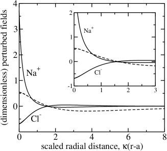
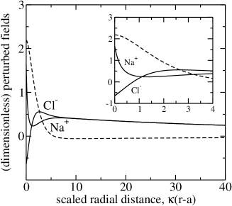
Figure 2: The structure of the perturbed double layer—under the influence of a bulk electrolyte concentration gradient—as revealed by the (scaled) radial electrostatic potential, $\hat{\psi}(r)2Ie/(kTa)$ (dashed lines), and ion concentration, $\hat{n}_{1}(r)/a$ (Na⁺) and $\hat{n}_{2}(r)/a$ (Cl⁺) (solid lines), perturbations (see Eqns. (14)–(16)) as a function of the (scaled) radial position $\kappa(r-a)$: aqueous NaCl at $T=25$^∘C; $a=100$ nm; ${\ell}\approx 3.11$ nm; $(\kappa a,\zeta e/(kT))=(1,-2)$ (left panel); $(\kappa a,\zeta e/(kT))=(100,-2)$ (right panel).

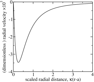
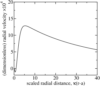
Figure 3: The structure of the perturbed double layer—under the influence of a bulk electrolyte concentration gradient—as revealed by the (dimensionless) radial velocity $-2(h_{r}/r)2I/(u^{*}a)$ ($u^{*}=\epsilon_{s}\epsilon_{o}(kT/e)^{2}/(\eta a)\approx 5.15\times 10^{-3}$ m s^-1) (see Eqn. (16)) as a function of the (scaled) radial position $\kappa(r-a)$. Parameters are the same as in figure 2.

For a composite with a relatively large Brinkman screening length ${\ell}\approx 9.95$ nm, the concentration-gradient-induced pore velocities shown in figure 4 are low. As expected, the incremental pore mobility increases with the surface charge (or $\zeta$-potential) and Darcy permeability. The mobility is shown in figure 5 as a function of the Brinkman screening length for various $\zeta$-potentials, with an ionic strength $I\approx 0.0925$ mol l^-1 yielding $\kappa a=100$. The direction of the concentration-gradient-induced flow is consistent with the discussion of table 1. Increasing the gel permeability strengthens the (forward flowing) electroosmotic flow in the outer region of the perturbed double layers and, hence, increases the bulk convective flow.

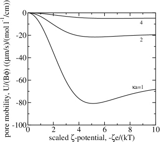
Figure 4: The incremental pore mobility $U/(B_{k^{\prime}}\phi)=-3C^{B_{k^{\prime}}}/a^{3}$ as a function of the (scaled) $\zeta$-potential $\zeta e/(kT)$ for (scaled) reciprocal double-layer thicknesses $\kappa a=1$, 2 and 4: aqueous NaCl at $T=25$^∘C; $a=100$ nm; ${\ell}\approx 9.95$ nm. An average concentration gradient is applied in the absence of average pressure and electrostatic potential gradients.

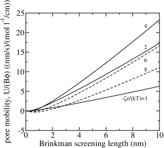
Figure 5: The incremental pore mobility $U/(B_{k^{\prime}}\phi)=-3C^{B_{k^{\prime}}}/a^{3}$ as a function of the Brinkman screening length ${\ell}$ for various (scaled) $\zeta$-potentials $-\zeta e/(kT)=1$, $2$, $4$ (solid lines) $6$ and $8$ (dashed lines): aqueous NaCl at $T=25$^∘C; $a=100$ nm; $\kappa a=100$; $I\approx 0.0925$ mol l^-1. An average concentration gradient is applied in the absence of average pressure and electrostatic potential gradients.

Contributions to the incremental fluxes are provided in table 2 for the composite whose asymptotic coefficients are listed in table 1. The first term on the right-hand side of Eqn. (28) (also columns 2 and 3 of table 2) is due to electromigration arising from concentration-gradient-induced electrical polarization. Polarization of (negatively) charged inclusions evidently enhances the effective diffusivity of the counter-ion (Na⁺) and attenuates that of the co-ion (Cl^-). The second term in Eqn. (28) (column 4 of the table) is due to diffusion, and arises from perturbations to the ion concentration gradients. As expected, this attenuates the diffusive flux when the $\zeta$-potential is moderate, and approaches the Maxwell value $\Delta_{j,d}^{B_{k^{\prime}}}=-3/2$ as $|\zeta|\rightarrow 0$. The last term in Eqn. (28) (also column 5) is due to electroosmotic flow (convection). This diminishes the fluxes of both ions, but its contribution is relatively small. Summing all three contributions (last two columns) shows that the average diffusive flux of the co-ion (Cl^-) is attenuated by the inclusions, most significantly at low ionic strength when electrostatic screening of the surface charge is weak. Similarly, the flux of the counter-ion (Na⁺) is enhanced because of electromigration. Again, when electrical forces are weak, the inclusions simply hinder diffusion and $\Delta_{j}^{B_{k^{\prime}}}\rightarrow-3/2$ as $|\zeta|\rightarrow 0$.

Table 2: Scaled asymptotic coefficients and microscale incremental contributions (see text) to average diffusion of NaCl in a Brinkman medium with charged spherical inclusions: $a=100$ nm; ${\ell}\approx 0.951$ nm; $T=25$^∘C; $D_{1}\approx 1.33\times 10^{-9}$m²s^-1 (Na⁺); $D_{2}\approx 2.03\times 10^{-9}$m²s^-1 (Cl^-).

$\zeta e/(kT)$	$\Delta_{1,e}^{B_{k^{\prime}}}$ (Na+) ($=-\Delta_{2,e}^{B_{k^{\prime}}}$)	$\Delta_{j,d}^{B_{k^{\prime}}}$ ($j=1,2$)	$\Delta_{1,c}^{B_{k^{\prime}}}$ (Na+)	$\Delta_{2,c}^{B_{k^{\prime}}}$ (Cl-)	$\Delta_{1}^{B_{k^{\prime}}}$ (Na+)	$\Delta_{2}^{B_{k^{\prime}}}$ (Cl-)
$\kappa a=1$	$I=9.25\times 10^{-6}$ mol l-1
$-1$	$6.25\times 10^{0}$	$-1.15\times 10^{0}$	$-8.76\times 10^{-6}$	$-5.74\times 10^{-6}$	$5.10\times 10^{0}$	$-7.39\times 10^{0}$
$-2$	$1.22\times 10^{1}$	$-1.71\times 10^{-1}$	$-3.02\times 10^{-5}$	$-1.98\times 10^{-5}$	$1.21\times 10^{1}$	$-1.24\times 10^{1}$
$-4$	$2.23\times 10^{1}$	$+2.60\times 10^{0}$	$-6.61\times 10^{-5}$	$-4.34\times 10^{-5}$	$2.49\times 10^{1}$	$-1.97\times 10^{1}$
$-6$	$2.86\times 10^{1}$	$+4.79\times 10^{0}$	$-6.61\times 10^{-5}$	$-4.33\times 10^{-5}$	$3.34\times 10^{1}$	$-2.39\times 10^{1}$
$-8$	$3.17\times 10^{1}$	$+5.89\times 10^{0}$	$-5.66\times 10^{-5}$	$-3.71\times 10^{-5}$	$3.75\times 10^{1}$	$-2.58\times 10^{1}$
$\kappa a=10$	$I=9.25\times 10^{-4}$ mol l-1
$-1$	$4.38\times 10^{-1}$	$-1.42\times 10^{0}$	$-1.47\times 10^{-5}$	$-9.65\times 10^{-6}$	$-9.84\times 10^{-1}$	$-1.86\times 10^{0}$
$-2$	$9.07\times 10^{-1}$	$-1.19\times 10^{0}$	$-5.79\times 10^{-5}$	$-3.80\times 10^{-5}$	$-2.88\times 10^{-1}$	$-2.10\times 10^{0}$
$-4$	$1.94\times 10^{0}$	$-4.25\times 10^{-1}$	$-1.77\times 10^{-4}$	$-1.16\times 10^{-4}$	$+1.51\times 10^{0}$	$-2.36\times 10^{0}$
$-6$	$2.82\times 10^{0}$	$+3.61\times 10^{-1}$	$-2.39\times 10^{-4}$	$-1.57\times 10^{-4}$	$+3.19\times 10^{0}$	$-2.46\times 10^{0}$
$-8$	$3.35\times 10^{0}$	$+8.42\times 10^{-1}$	$-2.47\times 10^{-4}$	$-1.62\times 10^{-4}$	$+4.19\times 10^{0}$	$-2.50\times 10^{0}$
$\kappa a=100$	$I=9.25\times 10^{-2}$ mol l-1
$-1$	$4.63\times 10^{-2}$	$-1.49\times 10^{0}$	$+1.75\times 10^{-4}$	$+1.14\times 10^{-4}$	$-1.44\times 10^{0}$	$-1.54\times 10^{0}$
$-2$	$1.03\times 10^{-1}$	$-1.45\times 10^{0}$	$+4.47\times 10^{-4}$	$+2.93\times 10^{-4}$	$-1.35\times 10^{0}$	$-1.56\times 10^{0}$
$-4$	$2.95\times 10^{-1}$	$-1.28\times 10^{0}$	$+3.98\times 10^{-4}$	$+2.61\times 10^{-4}$	$-9.88\times 10^{-1}$	$-1.58\times 10^{0}$
$-6$	$6.74\times 10^{-1}$	$-9.13\times 10^{-1}$	$+1.77\times 10^{-5}$	$+1.16\times 10^{-5}$	$-2.39\times 10^{-1}$	$-1.59\times 10^{0}$
$-8$	$1.24\times 10^{0}$	$-3.53\times 10^{-1}$	$-1.82\times 10^{-4}$	$-1.20\times 10^{-4}$	$+8.83\times 10^{-1}$	$-1.59\times 10^{0}$

Effective diffusivity increments are shown in figure 6 as a function of the $\zeta$-potential for various values of $\kappa a$. Clearly, increasing the surface charge increases the effective diffusivity of the counter-ion (left panel) and decreases the diffusivity of the co-ion (right panel). Note that the calculations are insensitive to the gel permeability, so these results are applicable to a variety of composites with negatively charged inclusions and NaCl electrolyte. In general, all bulk properties that reflect concentration and electrical polarization are independent of the Darcy permeability.

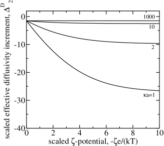
Figure 6: The (scaled) effective diffusivity increments $\Delta_{j}^{D}=(D_{j}^{*}/D_{j}-1)/\phi$ for Na⁺ (left panel) and Cl^- (right panel) as a function of the (scaled) $\zeta$-potential $\zeta e/(kT)$ with various (scaled) reciprocal double-layer thicknesses $\kappa a=1$, 2, 10, 100 and 1000 (aqueous NaCl at $T=25$^∘C with $a=100$ nm). Note that results are insensitive to the permeability ${\ell}^{2}$ of the polymer gel.

III.2 Bulk diffusion and electromigration

Having examined the application of an electrolyte concentration gradient in the absence of an electric field, let us now consider the electric field strength and concentration gradient that together yield zero current density. This ensures that transport of ions from one reservoir to another (with different electrolyte concentration) maintains electrical neutrality across a membrane. As expected from the previous section, an electric field is necessary to compensate for the lower (higher) diffusive flux of the less (more) mobile ion.

The analysis below is limited to situations where the bulk electrolyte concentration gradient is weak, permitting macroscale variations in the bulk equilibrium electrolyte concentration to be neglected. Complications that arise from macroscale variations in ion density, which are necessary to satisfy (bulk) continuity and electroneutrality constraints, will be addressed in future work; these are discussed briefly in §IV.

For the simple case involving the concentration gradient of a single $z$-$z$ electrolyte ($B_{j}=B_{k^{\prime}}$, $N=2$ and $M=1$), setting the current density (Eqn. (30)) to zero gives

$$\mbox{\boldmath$E$\unboldmath}K^{\infty}=\mbox{\boldmath$B$\unboldmath}_{k^{\prime}}\sum_{j=1}^{N=2}z_{j}eD_{j}(1+\phi\Delta^{E})+O(\phi^{2}),$$ (35)

where

$$\Delta^{E}\approx-(3/a^{3})[D^{B_{k^{\prime}}}\frac{K^{\infty}}{\sum_{j^{\prime}=1}^{N=2}z_{j^{\prime}}eD_{j^{\prime}}}+C_{j}^{B_{k^{\prime}}}+D^{E}+C_{j}^{E}\frac{\sum_{j^{\prime}=1}^{N=2}z_{j^{\prime}}eD_{j^{\prime}}}{K^{\infty}}]+O(\phi)$$ (36)

is termed the (dimensionless) electric-field increment. Note that $C_{j}^{E}$ and $C_{j}^{B_{k^{\prime}}}$ are independent of $j$, so $\Delta^{E}$ is independent of the sum in Eqn. (35).

Similarly to the concentration-gradient-induced current density (Eqn. 30), the $O(1)$ average electric field is zero for $z$-$z$ electrolytes whose ions have equal mobilities. It is important to note that the $O(\phi)$ contribution is not zero, however, even for perfectly symmetrical electrolytes. This follows from the influence of charged inclusions on the effective ion diffusivities, and emerges from Eqn. (36) through the term involving the gradient-induced electrostatic dipole strength $D^{B_{k^{\prime}}}$. Therefore, for a $z$-$z$ electrolyte whose ions have equal diffusivities $D_{j}$, Eqn. (35) simplifies to

$$\mbox{\boldmath$E$\unboldmath}=-\phi(3/a^{3})D^{B_{k^{\prime}}}\mbox{\boldmath$B$\unboldmath}_{k^{\prime}}+O(\phi^{2}),$$ (37)

showing that the average electric field reflects a sum of concentration-gradient-induced electrostatic dipole moments. In an homogeneous membrane, the membrane diffusion potential $\Delta\psi=\psi(z=L)-\psi(0)=-EL=\phi(3/a^{3})D^{B_{k^{\prime}}}B_{k^{\prime}}L$ is simply proportional to the concentration differential $B_{k^{\prime}}L$.

The electric-field increment is shown in figure 7 as a function of the $\zeta$-potential for various bulk ionic strengths yielding $\kappa a$ in the range 1–$10^{3}$. Again, because the increment reflects electrical and concentration polarization, the calculations are insensitive to flow and, hence, Darcy permeability. Therefore, the results are applicable to a variety of composites with negatively charged inclusions and NaCl electrolyte. Note that the increment is large at low ionic strength (small $\kappa a$) when the $\zeta$-potential is high, so the particle contribution may be comparable to or greater than that of the electrolyte alone. Further, when $\Delta^{E}<0$, there exists an inclusion volume fraction

$$\phi^{*}=-1/\Delta^{E}$$ (38)

that yields zero electric field strength with any (weak) bulk electrolyte concentration gradient. Clearly, $\phi^{*}$ must be less than one to be consistent with assumptions underlying the theory. In turn, this limits the accuracy of such a prediction to situations where $-\Delta^{E}\sim\phi^{-1}$ ($\phi\ll 1$), which is achieved at low ionic strength (e.g., $\kappa a=1$ in figure 7).

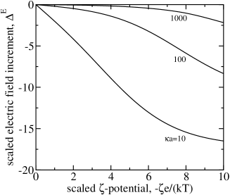
Figure 7: The (scaled) electric-field increment $\Delta^{E}$ (see Eqns. (35)–(36)) as a function of the (scaled) $\zeta$-potential $-\zeta e/(kT)$ for various (scaled) reciprocal double-layer thicknesses $\kappa a=1$, 2, 10, 100 and 1000: aqueous NaCl at $T=25$^∘C; $a=100$ nm. Note that the results are insensitive to the permeability ${\ell}^{2}$ of the polymer gel.

IV Summary

This paper demonstrates that a weak electrolyte concentration gradient applied across a permeable membrane hosting immobile charged inclusions induces bulk electroosmotic (or “diffusioosmotic”) flow. The direction of this flow may be up or down the concentration gradient, depending on the surface charge, bulk ionic strength, and permeability of the polymer gel. The inclusions also influence the ion fluxes or, equivalently, the effective ion diffusion coefficients. In short, the net counter-ion flux is enhanced by electromigration within the diffuse double layers.

Steady or quasi-steady transport across a membrane often takes place with zero current density, so, in practice, an external electric field—or an electric field from a macroscale redistribution of space charge—is necessary to maintain electrical neutrality. This work established the proportionality between this electric field and the imposed concentration gradient. It is tempting to attribute the strength of the electric field to electrolyte asymmetry alone, concluding, for example, that a perfectly symmetrical electrolyte will not produce a membrane diffusion potential. However, it was demonstrated that charged inclusions break the (effective) symmetry, so even a perfectly symmetrical electrolyte will yield a membrane diffusion potential. For NaCl (a moderately asymmetric $z$-$z$ electrolyte) in the presence of negatively charged inclusions, the electric-field increment is negative, so the diffusion potential of the composite is lower than in the absence of inclusions.

It should be emphasized that the present theory is limited to homogeneous membranes. Therefore, with a macroscopic length scale $L$ (e.g., membrane thickness), the differential concentrations $\Delta n_{j}^{\infty}=B_{j}L$ should be small relative to the bulk concentrations $n_{j}^{\infty}$. Even in the absence of inclusions, the bulk electrolyte fluxes are not straightforward to calculate without adopting one of the two following approximations. One consequence of electrical neutrality is that the electric field (e.g., with unidirectional transport) must be uniform. Similarly, ion conservation at steady state demands constant ion fluxes. However, solving the ion transport equations under these conditions leads to ion concentration fields that do not yield an electrically neutral bulk. This is the scenario that underlies the Goldman-Hodgkin-Katz (GHK) equation, which is well known in membrane biology (Sten-Knudsen:2002, ). An alternative approach constrains the ion concentration fields to ensure electrical neutrality. Then, however, the (bulk) ion fluxes are not uniform and, hence, the ion concentrations cannot be steady. This scenario underlies the Henderson equation, which is well known in electrochemistry and electrochemical engineering (Sten-Knudsen:2002, ). It is interesting to note that both theories yield the same membrane diffusion potential $\Delta\psi=\psi(z=L)-\psi(0)=-EL$ when the equations are linearized for small electrostatic potentials $\psi<kT/e$. Given the difficulties in solving coupled electromigration and diffusion (electro-diffusion) in the absence of inclusions, the problem with charged inclusions seems intractable at present. This work will hopefully stimulate further work in this area.

- (1) J. L. Anderson. Colloidal transport by interfacial forces. Ann. Rev. Fluid Mech., 21:61–99, 1989.
- (2) F. Booth. The cataphoresis of spherical, solid non-conducting particles in a symmetrical electrolyte. Proc. Roy. Soc. Lond., 203:533–551, 1950.
- (3) H. C. Brinkman. A calculation of the viscous force exerted by a flowing fluid on a dense swarm of particles. Appl. Sci. Res. A, 1:27–34, 1947.
- (4) P. Debye and A. M. Bueche. Intrinsic viscosity, diffusion, and sedimentation rate of polymers in solution. J. Chem. Phys., 16(6):573–578, 1948.
- (5) S. S. Dukhin and B. V. Derjaguin. Electrokinetic Phenomena, volume 7 of Surface & Colloid Science. Wiley, New York, 1974.
- (6) R. Hagedorn, T. Schnelle, T. Müller, I. Scholz, K. Lange, and M. Reh. Electrophoresis in gel channels. Electrophoresis, 26:2495–2502, 2005.
- (7) R. J. Hill. Hydrodynamics and electrokinetics of spherical liposomes with coatings of terminally anchored poly(ethylene glycol): Numerically exact electrokinetics with self-consistent mean-field polymer. Phys. Rev. E, 70:051046, 2004.
- (8) R. J. Hill. Transport in polymer-gel composites: Theoretical methodology and response to an electric field. J. Fluid Mech. (In press), 2005.
- (9) R. J. Hill and D. A. Saville. ‘Exact’ solutions of the full electrokinetic model for soft spherical colloids: Electrophoretic mobility. Colloids and Surfaces A: Physicochem. Eng. Aspects, 267:31–49, 2005.
- (10) R. J. Hill, D. A. Saville, and W. B. Russel. Electrophoresis of spherical polymer-coated colloidal particles. J. Colloid Interface Sci., 258:56–74, 2003.
- (11) D. L. Koch and A. S. Sangani. Particle pressure and marginal stability limits for a homogeneous monodisperse gas fluidized bed: Kinetic theory and numerical simulations. J. Fluid Mech., 400:229–263, 1999.
- (12) N. Lakshminarayanaiah. Transport Phenomena in Membranes. Academic Press, 1969.
- (13) S. Levine, K. Levine, K. A. Sharp, and D. E. Brooks. Theory of the electrokinetic behavior of human erythrocytes. Biophys. J., 42:127–135, 1983.
- (14) R. W. O’Brien. The electrical conductivity of a dilute suspension of charged particles. J. Colloid Interface Sci., 81(1):234–248, 1981.
- (15) R. W. O’Brien and L. R. White. Electrophoretic mobility of a spherical colloidal particle. J. Chem. Soc., Faraday Trans. II, 74:1607–1626, 1978.
- (16) H. Ohshima. Approximate analytical expressions for the electrophoretic mobility of colloidal particles with surface-charge layers. J. Colloid Interface Sci., 130:281–282, 1989.
- (17) J. Th. G. Overbeek. Theorie der elektrophorese. Kolloid-Beih., 54:287–364, 1943.
- (18) D. C. Prieve, J. L. Anderson, J. P. Ebel, and M. E. Lowell. Motion of a particle generated by chemical gradients. Part 2. electrolytes. J. Fluid Mech., 148:247–269, 1984.
- (19) D. C. Prieve and R. Roman. Diffusiophoresis of a rigid sphere through a viscous electrolyte solution. J. Chem. Soc. Faraday Trans. 2, 83(8):1287–1306, 1987.
- (20) D. A. Saville. Electrical conductivity of suspensions of charged particles in ionic solutions. J. Colloid Interface. Sci., 71(3):477–490, 1979.
- (21) D. A. Saville. Electrokinetic properties of fuzzy colloidal particles. J. Colloid Interface Sci., 222:137–145, 2000.
- (22) O. Sten-Knudsen. Biological Membranes: Theory of transport potentials and electric impulses. Cambridge University Press, 2002.
- (23) Y. K. Wei and H. J. Keh. Theory of electrokinetic phenomena in fibrous porous media caused by gradients of electrolyte concentration. Colloids and Surfaces A: Physiochem. Eng. Aspects, 222:301–310, 2003.
- (24) R. W. Wunderlich. The effects of surface structure on the electrophoretic mobilities of large particles. J. Colloid Interface Sci., 88(2):385–397, 1982.