Spin, bond and global fluctuation-dissipation relations in the non-equilibrium spherical ferromagnet

Abstract

We study the out-of-equilibrium dynamics of the spherical ferromagnet after a quench to its critical temperature. We calculate correlation and response functions for spin observables which probe lengthscales much larger than the lattice spacing but smaller than the system size, and find that the asymptotic fluctuation-dissipation ratio (FDR) $X^{\infty}$ is the same as for local observables. This is consistent with our earlier results for the Ising model in dimension $d=1$ and $d=2$. We also check that bond observables, both local and long-range, give the same asymptotic FDR. In the second part of the paper the analysis is extended to global observables, which probe correlations among all $N$ spins. Here non-Gaussian fluctuations arising from the spherical constraint need to be accounted for, and we develop a systematic expansion in $1/\sqrt{N}$ to do this. Applying this to the global bond observable, i.e. the energy, we find that non-Gaussian corrections change its FDR to a nontrivial value which we calculate exactly for all dimensions $d>2$. Finally, we consider quenches from magnetized initial states. Here even the FDR for the global spin observable, i.e. the magnetization, is nontrivial. It differs from the one for unmagnetized states even in $d>4$, signalling the appearance of a distinct dynamical universality class of magnetized critical coarsening. For lower $d$ the FDR is irrational even to first order in $4-d$ and $d-2$, the latter in contrast to recent results for the $n$-vector model.

1 Introduction

A key insight of statistical mechanics is that equilibrium states can be accurately described in terms of only a small number of thermodynamic variables, such as temperature and pressure. For non-equilibrium systems such as glasses no similar simplification exists a priori; the whole past history of a sample is in principle required to specify its state at a given time. This complexity makes theoretical analysis awkward, and one is led instead to look for a description of non-equilibrium states in terms of a few effective thermodynamic parameters. Much work in recent years has focussed on one such parameter, the effective temperature. This can be defined on the basis of fluctuation-dissipation (FD) relations between correlation and response functions and has proved to be very fruitful in mean field systems [1, 2].

The use of FD relations to quantify the out-of-equilibrium dynamics in glassy systems is motivated by the occurrence of aging [3]: the time scale of response to an external perturbation increases with the age (time since preparation) $t_{\rm w}$ of the system. As a consequence, time translational invariance and the equilibrium fluctuation-dissipation theorem [4] (FDT) relating correlation and response functions break down. To quantify this, one considers the correlation function of two generic observable $A$ and $B$ of a system, defined as

$$C(t,t_{\rm w})=\left\langle A(t)B(t_{\rm w})\right\rangle-\left\langle A(t)\right\rangle\left\langle B(t_{\rm w})\right\rangle$$ (1.1)

The associated (impulse) response function can be defined as

$$R(t,t_{\rm w})=\left.\frac{\delta\left\langle A(t)\right\rangle}{\delta h_{B}(t_{\rm w})}\right|_{h_{B}=0}$$

and gives the linear response of $A$ at time $t$ to a small impulse in the field $h_{B}$ conjugate to $B$ at the earlier time $t_{\rm w}$. (The latter is normally thought of as a “waiting time” since preparation of the system at time 0.) Equivalently one can work with the susceptibility

$$\chi(t,t_{\rm w})=\int_{t_{\rm w}}^{t}\!dt^{\prime}\,R(t,t^{\prime})$$ (1.2)

which encodes the response of $A(t)$ to a small step $h_{B}(t)=h_{B}\Theta(t-t_{\rm w})$ in the field starting at $t_{\rm w}$. In equilibrium, FDT implies that $-\partial_{t_{\rm w}}\chi(t,t_{\rm w})=R(t,t_{\rm w})={T}^{-1}\partial_{t_{\rm w}}C(t,t_{\rm w})$. Out of equilibrium, the violation of FDT can be measured by an FD ratio (FDR), $X$, defined through [5, 6]

$$-\partial_{t_{\rm w}}\chi(t,t_{\rm w})=R(t,t_{\rm w})=\frac{X(t,t_{\rm w})}{T}\partial_{t_{\rm w}}C(t,t_{\rm w})$$ (1.3)

This implies that $X$ can be read off from the slope $-X/T$ of a parametric FD plot showing $\chi$ vs $C$, at fixed $t$ and with $t_{\rm w}$ as the curve parameter. This remains the case if both axes are normalized by the equal-time variance of $A$, $C(t,t)$, a procedure which is helpful in fixing the scale of the plot in situations where $C(t,t)$ varies significantly with time [7, 8]. In equilibrium, the FD plot is a straight line with slope $-1/T$.

In mean-field spin glasses [1, 5, 6] one finds that FD plots of autocorrelation and response of local spins and similar observables approach a limiting shape for large $t$. This is typically composed of two straight line segments. In the first of these one finds $X=1$, corresponding to quasi-equilibrium dynamics for time differences $t-t_{\rm w}$ that do not grow with the age of the system. The second line segment has $X<1$ and reflects the dynamics on aging timescales, i.e. time differences growing (in the simplest case linearly) with $t_{\rm w}$. One can use this to define a non-equilibrium effective temperature $T_{\rm eff}=T/X$, which has been shown to have many of the properties of a thermodynamic temperature [1, 5, 6].

How well this physically very attractive mean-field scenario transfers to more realistic non-equilibrium systems with short-range interactions has been a matter of intense research recently [2]. A useful class of systems for studying this question in detail is provided by ferromagnets quenched from high temperature to the critical temperature (see e.g. Refs. [9, 10] and the recent review [11]) or below. The system then coarsens – by the growth of domains with the equilibrium magnetization, for $T<T_{c}$ – and exhibits aging; in an infinite system equilibrium is never reached. The aging is clearly related to the growth of a lengthscale [12] (domain size for $T<T_{\rm c}$, or correlation length for $T=T_{\rm c}$), and this makes ferromagnets attractive “laboratory” systems for understanding general properties of non-equilibrium dynamics. They are of course not completely generic; compared to e.g. glasses they lack features such as thermal activation over energetic or entropic barriers.

We focus in this paper mostly on ferromagnets quenched to $T_{\rm c}$, i.e. on critical coarsening dynamics. Some care is needed in this case with the interpretation of limiting FD plots: while in the mean-field situation $X$ becomes at long times a function of $C$ only, as implied by the existence of a nontrivial limit plot, in critical coarsening $X$ approaches a function of $t/t_{\rm w}$ [9]. In the interesting regime where $t/t_{\rm w}$ is finite but $>1$, time differences $t-t_{\rm w}={{\mathcal{O}}}(t_{\rm w})$ are then large, and e.g. spin autocorrelation functions have decayed to a small part of their initial value. In the limit $t,t_{\rm w}\to\infty$ the FD plot then assumes a pseudo-equilibrium shape, with all nontrivial detail compressed into a vanishing region around $C=0$.

The fact that the FDR is a smooth function of $t/t_{\rm w}$ makes the interpretation of $T/X$ as an effective temperature less obvious than in mean-field spin glasses, where $T/X$ is constant within each time sector ($t-t_{\rm w}={{\mathcal{O}}}(1)$ vs $t-t_{\rm w}$ growing with $t_{\rm w}$). To eliminate the time-dependence one can consider the limit of times that are both large and well-separated. This defines an asymptotic FDR

$$X^{\infty}=\lim_{t_{\rm w}\to\infty}\lim_{t\to\infty}X(t,t_{\rm w})$$ (1.4)

An important property of this quantity is that it should be universal [9, 11] in the sense that its value is the same for different systems falling into the same universality class of critical non-equilibrium dynamics. This makes a study of $X^{\infty}$ interesting in its own right, even without an interpretation in terms of effective temperatures.

If one nevertheless wants to pursue such an interpretation, the resulting value of the effective temperature $T/X^{\infty}$ should be the same for all (or at least a large class of) observables $A$. The observable-dependence of $X^{\infty}$ therefore becomes a key question [7, 8, 10, 13]. Conventionally, much work on non-equilibrium ferromagnets has focussed on the local spin autocorrelation function and associated response. An obvious alternative is the long-wavelength analogue, i.e. the correlation function of the fluctuating magnetization. Exact calculations for the Ising chain [10, 14] as well as numerical simulations [10, 15] in dimension $d=2$ show that the resulting global $X^{\infty}$ is always identical to the local version. This local–global correspondence, which can also be obtained by field-theoretic arguments [11, 16, 17], arises physically because the long wavelength Fourier components of the spins are slowest to relax and dominate the long-time behaviour of both local and global quantities.

The local–global correspondence does of course not address the full range of observable-dependence of the asymptotic FDR; one might ask about other observables which are linear combinations not of spins but for example products of interacting spins. In the critical Ising model in $d=2$, numerical simulations [10, 15] suggest that even these give the same $X^{\infty}$, so that an interpretation of $T/X^{\infty}$ in terms of an effective temperature appears plausible. One of the motivations for the current study was to verify whether this observable-independence of $X^{\infty}$ across different types of observables holds in an exactly solvable model, the spherical ferromagnet [18, 19]. In addition, we will study what effect different initial conditions have on $X^{\infty}$. This is motivated by our recent study of Ising models in the classical regime of large $d$, where critical fluctuations are irrelevant [20]. It turned out that magnetized initial do states produce a different value of $X^{\infty}$, so that critical coarsening in the presence of a nonzero magnetization is in a new dynamical universality class even though the magnetization does decay to zero at long times.

We begin in Sec. 2 with a brief review of the standard setup for the dynamics of the spherical model, as used in e.g. [9]. Fluctuations in an effective Lagrange multiplier enforcing the spherical constraint are neglected, leading to a theory where all spins are Gaussian random variables. In Sec. 3 this is applied to various observables of finite range, by which we mean correlations and responses probing lengthscales that can be large but remain small compared to the overall system size. For spin observables we show that the expected equality of $X^{\infty}$ between local and long-range quantities holds (Sec. 3.1). We check observable-independence of $X^{\infty}$ further by considering bond and spin product observables, in Sec. 3.2 and 3.3 respectively.

The major part of the paper is then devoted to a study of FDRs for global observables, with a focus on the energy, i.e. the global bond observable. Because of the weak infinite-range interaction generated by the spherical constraint, such observables behave differently from their long-range analogues in the spherical model. Calculations of correlation and response functions are technically substantially more difficult because Lagrange multiplier fluctuations can no longer be neglected. To account for them we construct in Sec. 4 a systematic expansion of the dynamically evolving spins in $N^{-1/2}$. This allows us to calculate the leading non-Gaussian corrections that we need for global correlations, as shown for the case of the energy in Sec. 5. After a brief digression to equilibrium dynamics, we evaluate the resulting expressions in Sec. 6 for $d$ above the critical dimension $d_{\rm c}=4$, and in Sec. 7 for $d<4$. Importantly, we will find that in the latter case the asymptotic FDR is different from those for finite-range observable. This means that an effective temperature interpretation of $X^{\infty}$ is possible at best in a very restricted sense. However, we will find that our results are in agreement with recent renormalization group (RG) calculations near $d=4$ [13] in the $O(n\to\infty)$-model. This suggests that the non-Gaussian effects captured in global observables are important for linking the spherical model to more realistic systems with only short-range interactions. Finally, we turn in Sec. 8 to critical coarsening starting from magnetized initial conditions. Here already the global spin observable is affected by non-Gaussian corrections. Once these are accounted for, we find $X^{\infty}=4/5$ for $d>4$ as in the Ising case [20]. For $d<4$ we provide the first exact values of the asymptotic FDR in the presence of a nonzero magnetization; these turn out to be highly nontrivial even to first order in $4-d$ and $d-2$. Our results are summarized and discussed in Sec. 9. Technical details are relegated to two appendices.

2 Langevin dynamics and Gaussian theory

We consider the standard spherical model Hamiltonian

$$H=\frac{1}{2}\sum_{(ij)}(S_{i}-S_{j})^{2}$$ (2.1)

The sum runs over all nearest neighbour (n.n.) pairs on a $d$-dimensional (hyper-)cubic lattice; the lattice constant is taken as the unit length. At each of the $N$ lattice sites $\mathbf{r}_{i}$ there is a real-valued spin $S_{i}$. The spherical constraint $\sum_{i}S_{i}^{2}=N$ is imposed, which can be motivated by analogy with Ising spins $S_{i}=\pm 1$ [18].

The Langevin dynamics for this model can be written as

$$\partial_{t}S_{i}=-\frac{\partial H}{\partial S_{i}}+\xi_{i}-\frac{1}{N}\sum_{k}S_{k}\left(-\frac{\partial H}{\partial S_{k}}+\xi_{k}\right)S_{i}$$ (2.2)

with $\xi_{i}$ Gaussian white noise with zero mean and covariance $\left\langle\xi_{i}(t)\xi_{j}(t^{\prime})\right\rangle=2T\delta_{ij}\delta(t-t^{\prime})$. The last term in (2.2), i.e. the sum over $k$, enforces the spherical constraint at all times by removing the component of the velocity vector $(\partial_{t}S_{1},\ldots,\partial_{t}S_{N})$ along $(S_{1},\ldots,S_{N})$. We use here the Stratonovic convention for products like $S_{k}\xi_{k}$. This allows the ordinary rules of calculus to be used when evaluating derivatives such as $\partial_{t}S_{i}^{2}$. Physically it corresponds to the intuitively reasonable scenario where the noise $\xi_{i}$ is regarded as a smooth random process but with a correlation time much shorter than any other dynamical timescale.

The prefactor of $S_{i}$ in the last term of (2.2), being an average of $N$ contributions, will have fluctuations of ${{\mathcal{O}}}(N^{-1/2})$. Conventionally one ignores these and approximates the equation of motion as

$$\partial_{t}S_{i}=-\frac{\partial H}{\partial S_{i}}+\xi_{i}-z(t)S_{i}$$ (2.3)

where $z(t)$ can be viewed as an effective time-dependent Lagrange multiplier implementing the spherical constraint. This approximation works for local quantities, but as we will see can give incorrect results when one considers e.g. fluctuations of the magnetization or the energy, which involve correlations across the entire system. One can see directly that (2.3) is an approximation from the fact that it corresponds to Langevin dynamics with the effective Hamiltonian $H+\frac{1}{2}z(t)\sum_{i}S_{i}^{2}$. Since the latter is time-dependent, this dynamics does not satisfy detailed balance. It is simple to check, on the other hand, that the original equation of motion (2.2) does satisfy detailed balance and leads to the correct equilibrium distribution $P_{\rm eq}(\{S_{i}\})\propto\exp(-\beta H)\delta(\sum S_{i}^{2}-N)$ where $\beta=1/T$ is the inverse temperature as usual.

The key advantage of the approximation (2.3) is, of course, that the spins are Gaussian random variables at all times as long as the initial condition is of this form. Explicitly, if we define a matrix $\Omega$ with $\Omega_{ij}=-1$ for n.n. sites $i,j$ and $\Omega_{ii}=2d$, the Gaussian equation of motion is

$$\partial_{t}S_{i}=-\sum_{j}\Omega_{ij}S_{j}-z(t)S_{i}+\xi_{i}$$ (2.4)

We review briefly how this is solved (see e.g. [9] and references therein), since these results form the basis for all later developments. In terms of the Fourier components $S_{\mathbf{q}}=\sum_{i}S_{i}\exp(-i\mathbf{q}\cdot\mathbf{r}_{i})$ of the spins, equation (2.4) reads

$$\partial_{t}S_{\mathbf{q}}=-(\omega_{\mathbf{q}}+z(t))S_{\mathbf{q}}+\xi_{\mathbf{q}}$$ (2.5)

where $\omega_{\mathbf{q}}=2\sum_{a=1}^{d}(1-\cos q_{a})$; we mostly write just $\omega$. The Fourier mode response function can be read off as

$$R_{\mathbf{q}}(t,t_{\rm w})=\exp\left(-\omega(t-t_{\rm w})-\int_{t_{\rm w}}^{t}dt^{\prime}\,z(t^{\prime})\right)\equiv\sqrt{\frac{g(t_{\rm w})}{g(t)}}e^{-\omega(t-t_{\rm w})}$$ (2.6)

where

$$g(t)=\exp\left(2\int_{0}^{t}dt^{\prime}\,z(t^{\prime})\right)$$ (2.7)

In terms of this, the time-dependence of the $S_{\mathbf{q}}$ becomes

$$S_{\mathbf{q}}(t)=R_{\mathbf{q}}(t,0)S_{\mathbf{q}}(0)+\int_{0}^{t}dt^{\prime}\,R_{\mathbf{q}}(t,t^{\prime})\xi_{\mathbf{q}}(t^{\prime})$$ (2.8)

The equal-time correlator $C_{\mathbf{q}}(t,t)=(1/N)\left\langle S_{\mathbf{q}}(t)S_{\mathbf{q}}^{*}(t)\right\rangle$ follows as

$$C_{\mathbf{q}}(t,t) = C_{\mathbf{q}}(0,0)R_{\mathbf{q}}^{2}(t,0)+2T\int_{0}^{t}dt^{\prime}\,R_{\mathbf{q}}^{2}(t,t^{\prime})$$ (2.9)

$$= \frac{C_{\mathbf{q}}(0,0)}{g(t)}e^{-2\omega t}+2T\int_{0}^{t}dt^{\prime}\,\frac{g(t^{\prime})}{g(t)}e^{-2\omega(t-t^{\prime})}$$ (2.10)

and we note for later the identity

$$\partial_{t}C_{\mathbf{q}}(t,t)=2T-\left(2\omega+\frac{g^{\prime}(t)}{g(t)}\right)C_{\mathbf{q}}(t,t)$$ (2.11)

The two-time correlator $C_{\mathbf{q}}(t,t_{\rm w})=(1/N)\left\langle S_{\mathbf{q}}(t)S_{\mathbf{q}}^{*}(t_{\rm w})\right\rangle$ can be deduced from the analogue of (2.8) for initial time $t_{\rm w}$

$$S_{\mathbf{q}}(t)=R_{\mathbf{q}}(t,t_{\rm w})S_{\mathbf{q}}(t_{\rm w})+\int_{t_{\rm w}}^{t}dt^{\prime}\,R_{\mathbf{q}}(t,t^{\prime})\xi_{\mathbf{q}}(t^{\prime})$$ (2.12)

as

$$C_{\mathbf{q}}(t,t_{\rm w})=R_{\mathbf{q}}(t,t_{\rm w})C_{\mathbf{q}}(t_{\rm w},t_{\rm w})$$ (2.13)

The position-dependent correlation and response functions $C_{ij}(t,t_{\rm w})$ and $R_{ij}(t,t_{\rm w})$ are then just the inverse Fourier transforms of $C_{\mathbf{q}}(t,t_{\rm w})$ and $R_{\mathbf{q}}(t,t_{\rm w})$, respectively, with $\mathbf{q}$ conjugate to $\mathbf{r}_{j}-\mathbf{r}_{i}$.

2.1 The function $g(t)$

The calculations outlined above show that the Gaussian dynamics is fully specified once the function $g(t)$ is known. The latter can be found from the spherical constraint, which imposes $\int(dq)\,C_{\mathbf{q}}(t,t)=1$. Here and below we abbreviate $(dq)\equiv d\mathbf{q}/(2\pi)^{d}$, where the integrals runs over the first Brillouin zone of the hypercubic lattice, i.e. $\mathbf{q}\in[-\pi,\pi]^{d}$. Using (2.10) this constraint gives an integral equation for $g(t)$:

$$g(t)=\int(dq)\,C_{\mathbf{q}}(0,0)e^{-2\omega t}+2T\int_{0}^{t}dt^{\prime}\,f(t-t^{\prime})g(t^{\prime})$$ (2.14)

where

$$f(t)=\int(dq)\,e^{-2\omega t}=[e^{-4t}I_{0}(4t)]^{d}\approx(8\pi t)^{-d/2}$$ (2.15)

Here $I_{0}$ denotes a modified Bessel function and the final expression gives the asymptotic behaviour for large $t$. In terms of Laplace transforms $\hat{g}(s)=\int_{0}^{\infty}dt\,\exp(-st)g(t)$, eq. (2.14) then has the solution

$$\hat{g}(s)=\frac{1}{1-2T\hat{f}(s)}\int(dq)\,\frac{C_{\mathbf{q}}(0,0)}{s+2\omega}$$ (2.16)

With the exception of Sec. 8, we focus in this paper on random initial conditions, $C_{\mathbf{q}}(0,0)=1$, corresponding to a quench at time $t=0$ from equilibrium at infinite temperature. In this case the $\mathbf{q}$-integral in the last equation is just $\hat{f}(s)$, so that

$$\hat{g}(s)=\frac{\hat{f}(s)}{1-2T\hat{f}(s)}$$ (2.17)

The asymptotics of the corresponding $g(t)$ are well known; see e.g. [9, 21]. For $T$ above the critical temperature $T_{\rm c}$, which is given by

$$T_{\rm c}^{-1}=2\hat{f}(0)=\int(dq)\,\frac{1}{\omega}$$ (2.18)

there is a pole in $\hat{g}(s)$ at $s=2z_{\rm eq}$. Here $z_{\rm eq}$ is found from the condition $2T\hat{f}(2z_{\rm eq})=1$ or

$$\int(dq)\,\frac{T}{z_{\rm eq}+\omega}=1$$ (2.19)

The presence of this pole tells us that $g(t)\sim\exp(2z_{\rm eq}t)$ for long times, implying that the Lagrange multiplier $z(t)$ approaches $z_{\rm eq}$ for $t\to\infty$. Correspondingly, the condition (2.19) is just the spherical constraint at equilibrium, bearing in mind that $C^{\rm eq}_{\mathbf{q}}(t,t)=T/(z_{\rm eq}+\omega)$ from (2.5). Because $\omega\approx q^{2}$ for small $q=|\mathbf{q}|$, the phase space factor in the $\mathbf{q}$-integrals is $(dq)\sim d\omega\,\omega^{d/2-1}$ for small $q$ or $\omega$. This shows that $T_{\rm c}$ as given by (2.18) vanishes as $d\to 2$ from above; consequently we will always restrict ourselves to dimensions $d$ above this lower critical dimension.

At criticality ($T=T_{\rm c}$), $z_{\rm eq}$ vanishes, and $g(t)$ therefore no longer grows exponentially; instead one finds [9, 21]

$$g(t)\sim t^{-\kappa},\quad\kappa=\left\{\begin{array}[]{lll}(4-d)/2&\mbox{for}&2<d<4\\ 0&\mbox{for}&d>4\end{array}\right.$$ (2.20)

It is this case, of a quench to the critical temperature, that we will concentrate on throughout most of this paper. This is because here the FDR has the most interesting behaviour.

We note briefly that, in principle, $\int(dq)\,$ should be written as $(1/N)\sum_{\mathbf{q}}$, with the sum running over all $\mathbf{q}$ whose components are integers in the range $-L/2\ldots-1,0,1,\ldots L/2-1$ (assuming $L$ is even) multiplied by an overall factor $2\pi/L$; there are $N$ such $\mathbf{q}$. When considering continuous functions of $\mathbf{q}$ this sum can be replaced by the integral $\int(dq)\,$, and this will almost always be the case in our analysis. Exceptions are situations with a nonzero magnetization, where the wavevector $\mathbf{q}=\mathbf{0}$ is special and has to be treated separately. This is relevant in equilibrium below $T_{\rm c}$, which we discuss briefly in Sec. 5.3, and for non-equilibrium dynamics starting from magnetized initial states (Sec. 8).

2.2 Long-time scaling of $C_{\mathbf{q}}$

It will be useful later to have a simplified long-time expression for $C_{\mathbf{q}}(t_{\rm w},t_{\rm w})$ for the case of a critical quench. At zero wavevector one has

$$C_{\mathbf{0}}(t_{\rm w},t_{\rm w})=\frac{1}{g(t_{\rm w})}\left(1+2T\int_{0}^{t_{\rm w}}dt^{\prime}\,g(t^{\prime})\right)\approx\frac{2Tt_{\rm w}}{1-\kappa}$$ (2.21)

where the last approximation is based on (2.20) and is valid for large $t_{\rm w}$. For nonzero $\mathbf{q}$, on the other hand,

$$C_{\mathbf{q}}(t_{\rm w},t_{\rm w})=\frac{1}{g(t_{\rm w})}\left(e^{-2\omega t_{\rm w}}+2T\int_{0}^{t_{\rm w}}dt^{\prime}\,g(t^{\prime})e^{-2\omega(t_{\rm w}-t^{\prime})}\right)\approx\frac{T}{\omega}$$ (2.22)

which is as expected since all nonzero Fourier modes eventually equilibrate. The crossover between the two limits takes place when $\omega t_{\rm w}\sim 1$, or $q\sim t_{\rm w}^{-1/2}$; physically this represents the growth of the time-dependent correlation length as $\sim t_{\rm w}^{1/2}$. We therefore introduce the scaling variable $w=\omega t_{\rm w}$:

$$\frac{C_{\mathbf{q}}(t_{\rm w},t_{\rm w})}{C_{\mathbf{0}}(t_{\rm w},t_{\rm w})}=\frac{e^{-2w}+2T\omega^{-1}\int_{0}^{w}dy\,g(y/\omega)e^{-2(w-y)}}{1+2T\omega^{-1}\int_{0}^{w}dy\,g(y/\omega)}$$ (2.23)

Now keep $w$ constant and let $t_{\rm w}\to\infty$, i.e. $\omega\to 0$. Then $g(y/\omega)\sim(y/\omega)^{-\kappa}$ and the second terms dominate in denumerator and nominator to give

$$\frac{C_{\mathbf{q}}(t_{\rm w},t_{\rm w})}{C_{\mathbf{0}}(t_{\rm w},t_{\rm w})}=(1-\kappa)\int_{0}^{1}dy\,y^{-\kappa}e^{-2w(1-y)}$$ (2.24)

Combining (2.24) with (2.21) then gives the desired long-time scaling form

$$C_{\mathbf{q}}(t_{\rm w},t_{\rm w})=\frac{T}{\omega}{\mathcal{F}}_{C}(\omega t_{\rm w}),\quad{\mathcal{F}}_{C}(w)=2w\int_{0}^{1}dy\,y^{-\kappa}e^{-2w(1-y)}$$ (2.25)

For $d>4$ ($\kappa=0$) this simplifies to ${\mathcal{F}}_{C}(w)=1-e^{-2w}$. As the derivation shows, eqs. (2.24) and (2.25) are valid whenever $t_{\rm w}\gg 1$, even for $\omega={{\mathcal{O}}}(1)$. The latter case corresponds to $w\to\infty$ and gives ${\mathcal{F}}_{C}(w)=1$, which is indeed consistent with (2.22).

For quantities such as $C_{\mathbf{q}}(t_{\rm w},t_{\rm w})$ that depend only on a single time variable, what is meant by the long-time limit is unambiguous. For two-time quantities like $C_{\mathbf{q}}(t,t_{\rm w})$ we use the following terminology: the long-time limit refers to the regime $t\gg 1$ and $t_{\rm w}\gg 1$ but without any restriction on $t-t_{\rm w}$, which in particular is allowed to be short, i.e. of ${{\mathcal{O}}}(1)$. The aging regime indicates more specifically the limit $t_{\rm w}\to\infty$ at fixed ratio $x=t/t_{\rm w}>1$, which implies that also $t-t_{\rm w}$ is large, of ${{\mathcal{O}}}(t_{\rm w})$. Occasionally we specialize further to the regime of well-separated times, which corresponds to $t\gg t_{\rm w}\gg 1$, i.e. the asymptotic behaviour of the aging limit for $x\gg 1$.

To illustrate the difference, consider which wavevectors dominate the integral $\int(dq)\,C_{\mathbf{q}}(t,t_{\rm w})$. In the long-time limit at equal times $t=t_{\rm w}$, the scaling $C_{\mathbf{q}}(t_{\rm w},t_{\rm w})\sim 1/\omega$ for $\omega\gg 1/t_{\rm w}$ combined with $(dq)\sim d\omega\,\omega^{d/2-1}$ for small $\omega$ shows that the integral is divergent at the upper end of the frequency regime $\omega={{\mathcal{O}}}(t_{\rm w}^{-1})$ for all $d>2$; in other words, it is always dominated by values of $\omega$ (and therefore $q$) of ${{\mathcal{O}}}(1)$. This remains true for two-time correlations, as long as $t-t_{\rm w}={{\mathcal{O}}}(1)$. In the aging limit, however, we have $t-t_{\rm w}={{\mathcal{O}}}(t_{\rm w})\gg 1$ and the exponential factor from $R_{\mathbf{q}}$ in (2.13) then ensures that only values of $\omega<(t-t_{\rm w})^{-1}={{\mathcal{O}}}(t_{\rm w}^{-1})$ have to be considered in the integral.

3 Fluctuation-dissipation relations for finite-range observables

In this section we consider FD relations for observables that probe correlations over a lengthscale that can be much larger than the lattice spacing, but remains much smaller than the system size. The latter can then be taken to infinity independently, so that the ${{\mathcal{O}}}(N^{-1/2})$-fluctuations of the Lagrange multiplier $z$ become irrelevant. We begin by considering briefly spin observables, and then discuss bond observables in some more detail.

3.1 Spin observables

Since all observables that are linear in the spins can be written as superpositions of the Fourier modes $S_{\mathbf{q}}$, the basic ingredient for understanding the FD behaviour is the FDR for the latter. Using (2.11), this follows after a couple of lines as ($C^{\prime}\equiv\partial_{t_{\rm w}}C$)

$$X_{\mathbf{q}}(t,t_{\rm w})=\frac{TR_{\mathbf{q}}(t,t_{\rm w})}{C^{\prime}_{\mathbf{q}}(t,t_{\rm w})}=T\left[2T-\left(\omega+\frac{g^{\prime}(t_{\rm w})}{2g(t_{\rm w})}\right)C_{\mathbf{q}}(t_{\rm w},t_{\rm w})\right]^{-1}$$ (3.1)

This is independent of the later time $t$, a feature that is commonly observed in simple non-equilibrium models [2].

The fluctuating magnetization is simply $S_{\mathbf{0}}/N$, so setting $\mathbf{q}=\mathbf{0}$ in (3.1) gives directly the FDR for the magnetization

$$X_{\mathbf{0}}(t,t_{\rm w})=T\left[2T-\frac{g^{\prime}(t_{\rm w})}{2g^{2}(t_{\rm w})}\left(1+2T\int_{0}^{t_{\rm w}}dt^{\prime}\,g(t^{\prime})\right)\right]^{-1}$$ (3.2)

As $t_{\rm w}$ increases this converges on an ${{\mathcal{O}}}(1)$ timescale to the limit-FDR

$$X^{\infty}=\frac{T}{2T+(\kappa/2)[2T/(1-\kappa)]}=\frac{1-\kappa}{2-\kappa}=\left\{\begin{array}[]{lll}1/2&(d>4)\\ 1-2/d&(d<4)\end{array}\right.$$ (3.3)

which is identical to the value obtained from the local magnetization [9] as one would expect on general grounds. Without working out the susceptibility explicitly, it is clear from the $t$-independence of $X_{\mathbf{0}}(t,t_{\rm w})$ and its fast convergence to $X^{\infty}$ that the limiting FD plot is a straight line. Both of these observations are exactly as in the Ising model in $d=1$ [10]. Simulations have shown that also in the $d=2$ Ising case the local–global correspondence holds for spin observables; the limiting FD plot is numerically indistinguishable from a straight line, though renormalization group arguments suggest that it should deviate slightly [15, 17, 11].

We should clarify that the Gaussian theory above applies directly not to the FDR for $S_{\mathbf{0}}$ but to the one for $S_{\mathbf{q}}$ with $q\ll t_{\rm w}^{-1/2}$ but $q\gg L^{-1}$, where $L=N^{1/d}$ is the linear system size. The corresponding physical observable is a “block” magnetization, i.e. the average of the spins within a block of size $\ell\sim 1/q$ much larger than the time-dependent correlation length $\sim t_{\rm w}^{1/2}$ but still small compared to the overall system size. For $\mathbf{q}=\mathbf{0}$, i.e. $\ell=L$, one would in principle need to account for the non-Gaussian fluctuations. However, it turns out that these are negligible as long as the system is not magnetized on average (see Sec. 8), so that the above results remain correct even for the global magnetization itself.

More generally, the FDR for any finite-range spin observable can be expressed as a superposition of those for the Fourier modes; this can be seen by arguments parallelling those in the $d=1$ Ising case [10]. As there, one can then show that the asymptotic FDR that is approached for well-separated times $t\gg t_{\rm w}\gg 1$ is dominated by the contribution from $\mathbf{q}=\mathbf{0}$, and hence identical to $X^{\infty}$ calculated above [11]. At equal times, on the other hand, equilibrated modes with $q={{\mathcal{O}}}(1)$ dominate and give $X=1$. The crossover between these two regimes takes place when $t-t_{\rm w}={{\mathcal{O}}}(t_{\rm w})$ and follows (by superposition) from the corresponding crossover at $q={{\mathcal{O}}}(t_{\rm w}^{-1})$ in the Fourier mode FDRs. From (2.25) and (3.1) the latter can be expressed as

$$X_{\mathbf{q}}(t,t_{\rm w})={\mathcal{F}}_{X}(\omega t_{\rm w}),\quad{\mathcal{F}}_{X}^{-1}(w)=2-(2w-\kappa)\int_{0}^{1}dy\,y^{-\kappa}e^{-2w(1-y)}$$ (3.4)

in the long-time limit, providing the expected interpolation between $X=X^{\infty}=1/[2+\kappa/(1-\kappa)]$ for $w\to 0$ and $X=1$ for $w\to\infty$.

3.2 Bond observables

Next we consider bond energy observables, $\frac{1}{2}(S_{i}-S_{j})^{2}$, where $i$ and $j$ are n.n. sites. Since all variables are Gaussian, the connected correlations follow by Wick’s theorem. For the correlation of bond energies one gets

$$C_{ij,kl}(t,t_{\rm w}) = 2\frac{1}{4}\left\langle[S_{i}(t)-S_{j}(t)][S_{k}(t_{\rm w})-S_{l}(t_{\rm w})]\right\rangle^{2}=\frac{1}{2}\left[C_{ik}-C_{il}-C_{jk}+C_{jl}\right]^{2}$$ (3.5)

where time arguments have been left implicit. For the local case $(i,j)=(k,l)$, this simplifies to

$$C_{ij,ij}=2[1-C_{ij}]^{2}$$ (3.6)

which tends to a nonzero constant for $t=t_{\rm w}\to\infty$ since $C_{ij}$ then approaches its equilibrium value, which is $<1$.

Next we turn to the response function. In general, if one perturbs the Hamiltonian $H$ by $-hB\delta(t-t_{\rm w})$, then the equation of motion for $S_{i}$ acquires an extra term $h(\partial B/\partial S_{i})\delta(t-t_{\rm w})$. So the perturbation in $S_{i}$ is

$$\delta S_{i}(t)=h\sum_{j}R_{ij}(t,t_{\rm w})\frac{\partial B}{\partial S_{j}}(t_{\rm w})$$ (3.7)

Thus the perturbation of an observable $A$ is

$$\delta A(t)=h\sum_{ij}\frac{\partial A}{\partial S_{i}}(t)R_{ij}(t,t_{\rm w})\frac{\partial B}{\partial S_{j}}(t_{\rm w})$$ (3.8)

giving the response function [13]

$$R_{AB}(t,t_{\rm w})=\sum_{ij}R_{ij}(t,t_{\rm w})\left\langle\frac{\partial A}{\partial S_{i}}(t)\frac{\partial B}{\partial S_{j}}(t_{\rm w})\right\rangle$$ (3.9)

For $A=\frac{1}{2}(S_{i}-S_{j})^{2}$, $B=\frac{1}{2}(S_{k}-S_{l})^{2}$ this yields

$$R_{ij,kl}(t,t_{\rm w})=[R_{ik}-R_{il}-R_{jk}+R_{jl}][C_{ik}-C_{il}-C_{jk}+C_{jl}]$$ (3.10)

We now analyse the scaling of correlation, response and the resulting FDR. In terms of $C_{\mathbf{q}}(t,t_{\rm w})$, the bond correlation (3.5) is

$$C_{ij,kl}(t,t_{\rm w})=\frac{1}{2}\left[\int(dq)\,C_{\mathbf{q}}\left(e^{i\mathbf{q}\cdot(\mathbf{r}_{i}-\mathbf{r}_{k})}-e^{i\mathbf{q}\cdot(\mathbf{r}_{i}-\mathbf{r}_{l})}-e^{i\mathbf{q}\cdot(\mathbf{r}_{j}-\mathbf{r}_{k})}+e^{i\mathbf{q}\cdot(\mathbf{r}_{j}-\mathbf{r}_{l})}\right)\right]^{2}$$ (3.11)

We can take out a factor $\exp(i\mathbf{q}\cdot\Delta\mathbf{r})$ from all the exponentials, where $\Delta\mathbf{r}=\frac{1}{2}(\mathbf{r}_{i}+\mathbf{r}_{j})+\frac{1}{2}(\mathbf{r}_{k}-\mathbf{r}_{l})$ is the distance vector between the bond midpoints. In the remaining exponentials, $\mathbf{q}$ is multiplied by vectors with lengths of order unity.

Now assume $t-t_{\rm w}\gg 1$. As explained above, integrals of two-time quantities over $\mathbf{q}$ are then dominated by the small-$q$ regime, $q^{2}\approx\omega<(t-t_{\rm w})^{-1}$. We can therefore Taylor expand in $\mathbf{q}$ and get, using the equivalence of the $d$ lattice directions,

$$C_{ij,kl}=\frac{1}{2}\left[d^{-1}(\mathbf{r}_{i}-\mathbf{r}_{j})\cdot(\mathbf{r}_{k}-\mathbf{r}_{l})\int(dq)\,C_{\mathbf{q}}q^{2}e^{i\mathbf{q}\cdot\Delta\mathbf{r}}\right]^{2}$$ (3.12)

Similarly one finds for the response

$$R_{ij,kl}=\left[d^{-1}(\mathbf{r}_{i}-\mathbf{r}_{j})\cdot(\mathbf{r}_{k}-\mathbf{r}_{l})\right]^{2}\int(dq)\,R_{\mathbf{q}}q^{2}e^{i\mathbf{q}\cdot\Delta\mathbf{r}}\int(dq)\,C_{\mathbf{q}}q^{2}e^{i\mathbf{q}\cdot\Delta\mathbf{r}}$$ (3.13)

For the local bond-bond correlation and response one sets $\Delta\mathbf{r}=\mathbf{0}$ and has $(\mathbf{r}_{i}-\mathbf{r}_{j})\cdot(\mathbf{r}_{i}-\mathbf{r}_{j})=1$, which gives for the FDR

$$X_{\rm bond}^{\rm loc}(t,t_{\rm w})=\frac{\int(dq)\,TR_{\mathbf{q}}q^{2}}{\int(dq)\,C^{\prime}_{\mathbf{q}}q^{2}}=\frac{\int(dq)\,R_{\mathbf{q}}q^{2}}{\int(dq)\,X^{-1}_{\mathbf{q}}R_{\mathbf{q}}q^{2}}$$ (3.14)

So $1/X_{\rm bond}^{\rm loc}(t,t_{\rm w})$ can be thought of as an average of $X_{\mathbf{q}}^{-1}(t,t_{\rm w})$ over $\mathbf{q}$, with the weight $R_{\mathbf{q}}(t,t_{\rm w})q^{-2}$. The factor $R_{\mathbf{q}}$ ensures that significant contributions come only from wavevectors $\mathbf{q}$ up to length $q\sim(t-t_{\rm w})^{-1/2}$, i.e. up to $\omega(t-t_{\rm w})\approx 1$. Thus, when $t-t_{\rm w}\ll t_{\rm w}$, the result is dominated by the regime $\omega t_{\rm w}\gg 1$, where $X_{\mathbf{q}}=1$. For $t-t_{\rm w}\gg t_{\rm w}$, meanwhile, one only gets contributions from $\omega t_{\rm w}\ll 1$, where $X_{\mathbf{q}}=X^{\infty}$. So the FDR (3.14) for local bond observables is a scaling function interpolating between $1$ and $X^{\infty}$, with the same $X^{\infty}$ as for the magnetization. Explicitly one has, using (2.6) and changing integration variable from $\mathbf{q}$ to $w=\omega t_{\rm w}$,

$$X_{\rm bond}^{\rm loc}(t,t_{\rm w})=\frac{\int_{0}^{\infty}dw\,w^{d/2}e^{-(x-1)w}}{\int_{0}^{\infty}dw\,w^{d/2}e^{-(x-1)w}{\mathcal{F}}_{X}^{-1}(w)}$$ (3.15)

with $x=t/t_{\rm w}$ and ${\mathcal{F}}_{X}$ the scaling form (3.4) of $X_{\mathbf{q}}$. To find the shape of the FD plot, recall that the equal-time value of the local-bond correlation (3.6) is a constant in the long-time limit. For $t-t_{\rm w}\gg 1$, on the other hand, eq. (3.12) shows that $C_{\rm bond}^{\rm loc}$ scales as

$$C_{\rm bond}^{\rm loc}(t,t_{\rm w}) \sim \frac{g(t_{\rm w})}{g(t)}\left[\int d\omega\,\omega^{d/2-1}\frac{T}{\omega}{\mathcal{F}}_{C}(\omega t_{\rm w})e^{-\omega(t-t_{\rm w})}\omega\right]^{2}$$ (3.16)

$$\sim \frac{g(t_{\rm w})}{g(t)}t_{\rm w}^{-d}\left[\int dw\,w^{d/2-1}{\mathcal{F}}_{C}(w)e^{-w(t-t_{\rm w})/t_{\rm w}}\right]^{2}$$ (3.17)

Since ${\mathcal{F}}_{C}(w)\to 1$ for $w\to\infty$, the $w$-integral would be divergent without the exponential cutoff and scales as $[(t-t_{\rm w})/t_{\rm w}]^{-d/2}$ for $t-t_{\rm w}\ll t_{\rm w}$, so that $C_{\rm bond}^{\rm loc}(t,t_{\rm w})\sim(t-t_{\rm w})^{-d}$ in this regime. The regime $t-t_{\rm w}>t_{\rm w}$ where $X_{\rm bond}^{\rm loc}(t,t_{\rm w})\neq 1$ is therefore compressed into the region where $C_{\rm bond}^{\rm loc}$ is of order $t_{\rm w}^{-d}$, so that the long-time limit of the FD plot is a straight line with equilibrium slope. Qualitatively one thus has the same behaviour as for local bond observables in the Ising model [10].

Next consider long-range bond observables, where we sum $(ij)$ and $(kl)$ over all bonds. The same proviso as above for the magnetization applies here, i.e. by applying the Gaussian theory we are effectively considering the bond energies averaged over a block that is large but has to remain nonetheless small compared to the system size. One can show that the resulting equal-time correlation again approaches a constant value for $t_{\rm w}\to\infty$. (This follows because for large $\Delta\mathbf{r}$, one can use the small $q$-expansion (3.12) even for equal times. From $C_{\mathbf{q}}(t_{\rm w},t_{\rm w})\approx T/q^{2}$ one gets $C(\Delta\mathbf{r};t_{\rm w},t_{\rm w})\sim|\Delta\mathbf{r}|^{2-d}$ for large $\Delta\mathbf{r}$ and so $\int(dq)\,C_{\mathbf{q}}q^{2}e^{i\mathbf{q}\cdot\Delta\mathbf{r}}\sim\nabla^{2}|\Delta\mathbf{r}|^{2-d}\sim|\Delta\mathbf{r}|^{-d}$. The square $|\Delta\mathbf{r}|^{-2d}$ then yields a convergent sum over $\Delta\mathbf{r}$.) So we focus directly on the regime $t-t_{\rm w}\gg 1$, where the expansion (3.12) is again valid. Keeping the bond $(ij)$ fixed, the scalar product $(\mathbf{r}_{i}-\mathbf{r}_{j})\cdot(\mathbf{r}_{k}-\mathbf{r}_{l})$ means that only bonds $(kl)$ parallel to $(ij)$ contribute, so that the sum over $(kl)$ becomes a sum over $\Delta\mathbf{r}$, running over all lattice vectors. (For non-parallel bonds, $\Delta\mathbf{r}$ could also assume other values not corresponding to lattice vectors.) The sum over $(ij)$ then just gives an overall factor of $Nd$. Normalizing by $N$, the block bond correlation function is

$$C_{\rm bond}^{\rm block}(t,t_{\rm w})=\frac{1}{2d}\frac{1}{N}\sum_{\Delta\mathbf{r}}\left[\int(dq)\,C_{\mathbf{q}}q^{2}e^{i\mathbf{q}\cdot\Delta\mathbf{r}}\right]^{2}=\frac{1}{2d}\int(dq)\,C^{2}_{\mathbf{q}}q^{4}$$ (3.18)

and similar arguments give for the (normalized) response

$$R_{\rm bond}^{\rm block}(t,t_{\rm w})=\frac{1}{d}\int(dq)\,R_{\mathbf{q}}C_{\mathbf{q}}q^{4}$$ (3.19)

so that the FDR becomes

$$X_{\rm bond}^{\rm block}(t,t_{\rm w})=\frac{\int(dq)\,TR_{\mathbf{q}}C_{\mathbf{q}}q^{4}}{\int(dq)\,C^{\prime}_{\mathbf{q}}C_{\mathbf{q}}q^{4}}=\frac{\int(dq)\,R_{\mathbf{q}}C_{\mathbf{q}}q^{4}}{\int(dq)\,X^{-1}_{\mathbf{q}}R_{\mathbf{q}}C_{\mathbf{q}}q^{4}}$$ (3.20)

Again, this is the inverse of a weighted average of $X^{-1}_{\mathbf{q}}$, now with weight $R_{\mathbf{q}}C_{\mathbf{q}}q^{4}$. The same arguments as for (3.14) then show that $X^{\rm block}(t,t_{\rm w})$ scales with $x=t/t_{\rm w}$ and interpolates between $X=1$ for $x=1$ and $X=X^{\infty}$ for $x\to\infty$. The value of the correlator (3.18) decays from ${{\mathcal{O}}}(1)$ at $t=t_{\rm w}$ to ${{\mathcal{O}}}(t_{\rm w}^{-d/2})$ at the point $x-1\approx 1$ where aging effects appear. While this is larger than for the local bond observables, it still decreases to zero for $t_{\rm w}\to\infty$, so that the limiting FD plot is again of pseudo-equilibrium form. This is different to the case of the Ising model, where the global bond observables give nontrivial limiting FD plots [10].

In more detail, the scaling of the block bond correlator (3.18) in the aging regime $t-t_{\rm w}\gg 1$ is

$$C_{\rm bond}^{\rm block}(t,t_{\rm w}) \sim \frac{g(t_{\rm w})}{g(t)}\int\!d\omega\,\omega^{d/2-1}\frac{T_{\rm c}^{2}}{\omega^{2}}{\mathcal{F}}_{C}^{2}(\omega t_{\rm w})e^{-2\omega(t-t_{\rm w})}\omega^{2}$$ (3.21)

$$\sim \left(\frac{t}{t_{\rm w}}\right)^{\kappa}t_{\rm w}^{-d/2}\int\!dw\,w^{d/2-1}{\mathcal{F}}_{C}^{2}(w)e^{-2(x-1)w}$$ (3.22)

The integral scales as $(x-1)^{-d/2}$ for $x\approx 1$, so $C_{\rm bond}^{\rm block}(t,t_{\rm w})\sim(t-t_{\rm w})^{-d/2}$ there. For $x\gg 1$, on the other hand, the integral becomes $\sim x^{-(d+4)/2}$, so $C_{\rm bond}^{\rm block}(t,t_{\rm w})\sim t_{\rm w}^{-\kappa+2}t^{\kappa-(d+4)/2}$. Explicitly, in this $t\gg t_{\rm w}$ regime, $C_{\rm bond}^{\rm block}\sim t_{\rm w}^{2}t^{-(d+4)/2}$ for $d>4$, and $C_{\rm bond}^{\rm block}\sim t_{\rm w}^{d/2}t^{-d}$ for $d<4$. The response function scales in the same way as $\partial_{t_{\rm w}}C_{\rm bond}^{\rm block}$, because $X$ is everywhere of order unity.

3.3 Product observables

Instead of the bond observables $\frac{1}{2}(S_{i}-S_{j})^{2}$ we could consider the spin products $A=S_{i}S_{j}$, $B=S_{k}S_{l}$. The correlations are then

$$C_{ij,kl}(t,t_{\rm w}) = \left\langle S_{i}(t)S_{j}(t)S_{k}(t_{\rm w})S_{l}(t_{\rm w})\right\rangle-\left\langle S_{i}(t)S_{j}(t)\right\rangle\left\langle S_{k}(t_{\rm w})S_{l}(t_{\rm w})\right\rangle$$ (3.23)

$$= C_{ik}(t,t_{\rm w})C_{jl}(t,t_{\rm w})+C_{il}(t,t_{\rm w})C_{jk}(t,t_{\rm w})$$ (3.24)

The local equal-time correlation function $C_{ij,ij}(t_{\rm w},t_{\rm w})$ thus approaches $2$ for $t_{\rm w}\to\infty$. The corresponding response function is

$$R_{ij,kl}(t,t_{\rm w})=R_{ik}C_{jl}+R_{il}C_{jk}+R_{jk}C_{il}+R_{jl}C_{ik}$$ (3.25)

In the local case, one can replace all functions by local ones in the aging regime – there are no cancellations leading to extra factors of $q^{2}$ as was the case for bond observables, compare e.g. (3.11) and (3.12) – so that the FDR

$$X_{\rm prod}^{\rm loc}(t,t_{\rm w})=\frac{4T_{\rm c}R_{ii}C_{ii}}{4C^{\prime}_{ii}C_{ii}}=\frac{T_{\rm c}R_{ii}}{C^{\prime}_{ii}}$$ (3.26)

becomes identical to the one for the spin autocorrelation and response. In particular, one again gets the same $X^{\infty}$.

For the global (block) case, we can write

$$C_{\rm prod}^{\rm block}(t,t_{\rm w}) = \sum_{(ij),(kl)}C_{ij,kl}(t,t_{\rm w})$$ (3.27)

$$= \frac{1}{4}\sum_{ijkl}n_{ij}n_{kl}\left[C_{ik}(t,t_{\rm w})C_{jl}(t,t_{\rm w})+C_{il}(t,t_{\rm w})C_{jk}(t,t_{\rm w})\right]$$ (3.28)

$$= \frac{1}{2}\sum_{ijkl}n_{ij}n_{kl}C_{ik}(t,t_{\rm w})C_{jl}(t,t_{\rm w})=\frac{1}{2}\int(dq)\,n^{2}_{\mathbf{q}}C_{\mathbf{q}}^{2}(t,t_{\rm w})$$ (3.29)

where $n_{ij}=1$ if $i$ and $j$ are nearest neighbours and 0 otherwise, and $n_{\mathbf{q}}$ is its Fourier transform. For the response one has similarly

$$R_{\rm prod}^{\rm block}(t,t_{\rm w})=\int(dq)\,n^{2}_{\mathbf{q}}R_{\mathbf{q}}(t,t_{\rm w})C_{\mathbf{q}}(t,t_{\rm w})$$ (3.30)

In the aging regime, where $t-t_{\rm w}\gg 1$, the integrals are dominated by small $q$, where $n_{\mathbf{q}}$ can be approximated by the constant $n_{\mathbf{0}}=2d$. This cancels from the FDR, which becomes

$$X_{\rm prod}^{\rm block}(t,t_{\rm w})=\frac{\int(dq)\,T_{\rm c}R_{\mathbf{q}}C_{\mathbf{q}}}{\int(dq)\,C^{\prime}_{\mathbf{q}}C_{\mathbf{q}}}$$ (3.31)

This is the inverse of the average of $X_{\mathbf{q}}^{-1}$ with weight $R_{\mathbf{q}}C_{\mathbf{q}}$. Again, this is a scaling function of $t/t_{\rm w}$ interpolating between $1$ and the same $X^{\infty}$ as for spin observables.

The scaling of the block product correlation function (3.29) itself is a little more complicated than for the bond observables and depends on dimensionality. Focussing again on $t-t_{\rm w}\gg 1$ one has $C_{\rm prod}^{\rm block}(t,t_{\rm w})\approx 2d^{2}\int(dq)\,C_{\mathbf{q}}^{2}(t,t_{\rm w})$. The integral defines the function $CC(t,t_{\rm w})$ discussed in Sec. 6 for $d>4$ and Sec. 7 for $d<4$. In the former case, one has from (6.8–6.10) that $CC(t,t_{\rm w})=CC_{\rm eq}(t-t_{\rm w}){\mathcal{F}}_{CC}(t/t_{\rm w})$ where $CC_{\rm eq}(t-t_{\rm w})\sim(t-t_{\rm w})^{(4-d)/2}$ asymptotically; this equilibrium contribution governs the behaviour of $C_{\rm prod}^{\rm block}(t,t_{\rm w})$ for $t-t_{\rm w}\ll t_{\rm w}$. Where aging effects appear ($t-t_{\rm w}\sim t_{\rm w}$), $C_{\rm prod}^{\rm block}\sim t_{\rm w}^{(4-d)/2}$ and so one gets a limiting pseudo-equilibrium FD plot. In the regime of well-separated times $x\gg 1$, the scaling function ${\mathcal{F}}_{CC}(x)$ decays as $x^{-2}$ so that $C_{\rm prod}^{\rm block}(t,t_{\rm w})\sim t_{\rm w}^{2}t^{-d/2}$. These scalings, though not the overall magnitude of $C_{\rm prod}^{\rm block}$, are the same as for the energy correlation function $C_{E}$ in (6.14) below: both functions are proportional to $CC(t,t_{\rm w})$ in the aging regime.

In the opposite case $d<4$, the equal-time value $CC(t,t)$ (and therefore $C_{\rm prod}^{\rm block}(t,t)$) diverges as $t^{(4-d)/2}$, see (7.4). The normalized correlator $CC(t,t_{\rm w})/CC(t,t)$ is a scaling function ${\mathcal{G}}(x)$ of $x=t/t_{\rm w}$, implying that the normalized FD plot will approach a nontrivial limit form, with asymptotic slope $X^{\infty}$ as shown above. Quantitatively, because ${\mathcal{G}}(x)\sim x^{-d/2}$ for $x\gg 1$, one has $C_{\rm prod}^{\rm block}(t,t_{\rm w})\sim t^{(4-d)/2}(t_{\rm w}/t)^{d/2}\sim t_{\rm w}^{d/2}t^{2-d}$ for $t\gg t_{\rm w}$.

4 Correlation and response for global observables

We now ask what happens if we go from block observables to truly global ones, which reflect properties averaged over the entire system; the total energy is an important example. We anticipate that here non-Gaussian fluctuations are important. Indeed, the results above show that this must be case. Otherwise we could directly extend the Gaussian theory results from block to global observables, with no change to correlation and response functions. The global bond observable is just the energy. Using the spherical constraint, this can be written as

$$E=\sum_{(ij)}\frac{1}{2}(S_{i}-S_{j})^{2}=N-\sum_{(ij)}S_{i}S_{j}$$ (4.1)

and so is identical to the global spin product observable, up to a trivial additive constant and sign. So the global bond and product observables must have identical correlation and response functions; but we saw above that this requirement is not satisfied by the Gaussian theory. Thus, non-Gaussian fluctuations are essential to get correct results for global observables.

Physically, the origin of the distinction between block observables and global ones is the effective infinite-range interaction induced by the spherical constraint. In a model with short-range interactions, block observables will show identical behaviour to global ones whenever the block size $\ell$ is larger than any correlation length in the system, whether or not $\ell\ll L$: the behaviour of any large subsystem is equivalent to that of the system as a whole. In the spherical model, the infinite-range interaction breaks this connection, and global correlation and response functions cannot be deduced from those for block observables.

4.1 Non-Gaussian fluctuations

To make progress, we need to return to the original equation of motion (2.2). This can be written as

$$\partial_{t}S_{i}=-\sum_{j}\Omega_{ij}S_{j}+\xi_{i}-(z(t)+N^{-1/2}\Delta z)S_{i}$$ (4.2)

where the notation emphasizes that the fluctuating contribution to the Lagrange multiplier is of ${{\mathcal{O}}}(N^{-1/2})$. The latter induces non-Gaussian fluctuations in the $S_{i}$ of the same order. This shows quantitatively why the Gaussian theory works for block observables: as long as one considers correlations of a number of spins that is $\ll N$, fluctuations of ${{\mathcal{O}}}(N^{-1/2})$ can be neglected. For global observables, on the other hand, we require the correlations of all $N$ spins and the Gaussian approximation then becomes invalid.

To account systematically for non-Gaussian effects we represent the spins as $S_{i}=s_{i}+N^{-1/2}r_{i}$, where $s_{i}$ gives the limiting result for $N\to\infty$, which has purely Gaussian statistics, and $N^{-1/2}r_{i}$ is a leading-order fluctuation correction which will be non-Gaussian. Inserting this decomposition into (4.2) and collecting terms of ${{\mathcal{O}}}(1)$ and ${{\mathcal{O}}}(N^{-1/2})$ gives $\partial_{t}s_{i}=-\Omega_{ij}s_{j}-z(t)s_{i}+\xi_{i}$ as expected; to lighten the notation we use the summation convention for repeated indices from now on. For the non-Gaussian corrections one gets the equation of motion

$$\partial_{t}r_{i}=-\Omega_{ij}r_{j}-z(t)r_{i}-\Delta z\,s_{i}$$ (4.3)

with solution

$$r_{i}(t)=R_{ij}(t,0)r_{j}(0)-\int_{0}^{t}dt^{\prime}\,R_{ij}(t,t^{\prime})s_{j}(t^{\prime})\Delta z(t^{\prime})$$ (4.4)

The properties of $\Delta z(t^{\prime})$ can now be determined from the requirement that, due to the spherical constraint, $N^{-1}\sum_{i}S^{2}_{i}(t)=1$ at all times. Inserting $S_{i}=s_{i}+N^{-1/2}r_{i}$ and expanding to the leading order in $N^{-1/2}$ gives the condition

$$\frac{1}{N}\sum_{i}s_{i}(t)r_{i}(t)=-\frac{1}{2}N^{-1/2}\sum_{i}(s_{i}^{2}(t)-1)\equiv-\frac{1}{2}\Delta(t)$$ (4.5)

where the last equality defines $\Delta(t)$, a fluctuating quantity of ${{\mathcal{O}}}(1)$ that describes the (normalized) fluctuations of the squared length of the Gaussian spin vector $s_{i}$. At $t=0$, the condition (4.5) is solved to leading order by setting $r_{i}(0)=-\frac{1}{2}\Delta(0)s_{i}(0)$, since $(1/N)\sum_{i}s_{i}^{2}(0)=1+{{\mathcal{O}}}(N^{-1/2})$. With this assignment, and setting $a(t)=2\Delta z(t)+\Delta(0)\delta(t)$, eq. (4.4) reads

$$r_{i}(t)=-\frac{1}{2}\int dt^{\prime}\,R_{ij}(t,t^{\prime})s_{j}(t^{\prime})a(t^{\prime})$$ (4.6)

We have left the integral limits unspecified here: the factor $R_{ij}$ automatically enforces $t^{\prime}<t$, and we use the convention $a(t^{\prime})=0$ for $t^{\prime}<0$. The spherical constraint condition (4.5) then becomes

$$\int dt^{\prime}\,\frac{1}{N}s_{i}(t)R_{ij}(t,t^{\prime})s_{j}(t^{\prime})a(t^{\prime})=\Delta(t)$$ (4.7)

Now, up to fluctuations of ${{\mathcal{O}}}(N^{-1/2})$ which are negligible to leading order (even if they are correlated with $a(t^{\prime})$), we can replace $(1/N)s_{i}(t)R_{ij}(t,t^{\prime})s_{j}(t^{\prime})$ by its average

$$K(t,t^{\prime})\equiv\frac{1}{N}\left\langle s_{i}(t)R_{ij}(t,t^{\prime})s_{j}(t^{\prime})\right\rangle=\frac{1}{N}R_{ij}(t,t^{\prime})C_{ij}(t,t^{\prime})=\int(dq)\,R_{\mathbf{q}}(t,t^{\prime})C_{\mathbf{q}}(t,t^{\prime})$$ (4.8)

If we then define the inverse operator, $L$, of $K$ via

$$\int dt^{\prime}\,K(t,t^{\prime})L(t^{\prime},t_{\rm w})=\delta(t-t_{\rm w})$$ (4.9)

for $t_{\rm w}\geq 0$, then the solution to (4.7) is

$$a(t)=\int dt^{\prime}\,L(t,t^{\prime})\Delta(t^{\prime})$$ (4.10)

where for consistency we adopt the convention $\Delta(t^{\prime})=0$ for $t^{\prime}<0$. With (4.6) we then get an explicit expression for the non-Gaussian ${{\mathcal{O}}}(N^{-1/2})$-corrections to the spins,

$$r_{i}(t)=-\frac{1}{2}\int dt^{\prime}dt^{\prime\prime}\,R_{ij}(t,t^{\prime})s_{j}(t^{\prime})L(t^{\prime},t^{\prime\prime})\Delta(t^{\prime\prime})$$ (4.11)

in terms of the properties of the uncorrected Gaussian spins $s_{i}$.

4.2 The functions $K$ and $L$

Before proceeding, we analyse the properties of $K$ and $L$. From (4.8), $K(t,t^{\prime})$ vanishes for $t<t^{\prime}$ while its limit value for $t\to t^{\prime+}$ is $(1/N)\delta_{ij}C_{ij}(t,t)=(1/N)C_{ii}(t,t)=1$. Inserting (2.6),  (2.11) and (2.13) into (4.8), one also finds that the equal-time slope has the simple value $\partial_{t^{\prime}}K\left.(t,t^{\prime})\right|_{t=t^{\prime+}}=2T$. From these properties and the definition (4.9) it follows that

$$L(t,t^{\prime})=\delta^{\prime}(t-t^{\prime})+L^{(1)}(t,t^{\prime}),\qquad L^{(1)}(t,t^{\prime})=2T\delta(t-t^{\prime})-L^{(2)}(t,t^{\prime})$$ (4.12)

where $L^{(2)}(t,t^{\prime})$ vanishes for $t<t^{\prime}$ and jumps to a finite value at $t=t^{\prime+}$; otherwise it is smooth and, as we will later see, positive. The structure of (4.12) can be easily verified e.g. for the limit of equilibrium at high temperature $T$, where $z_{\rm eq}=T$ and all $\omega$ can be neglected compared to $z_{\rm eq}$. One then has $K(t,t^{\prime})=\exp(-2T(t-t^{\prime}))$ and the inverse (4.9) can be calculated by Laplace transform. Since the Laplace transform of $K(t,t^{\prime})$ is $\hat{K}(s)=1/(s+2T)$ this gives $\hat{L}(s)=s+2T$, which corresponds to (4.12) with $L^{(2)}\equiv 0$.

We next determine the long-time forms of $K$ and $L^{(2)}$ for quenches to criticality. In both cases it is useful to factor out the equilibrium contribution. For $K$ this is, from (4.8) and using (2.6) and (2.13),

$$K_{\rm eq}(t-t_{\rm w})=\int(dq)\,e^{-2\omega(t-t_{\rm w})}\frac{T_{\rm c}}{\omega}$$ (4.13)

Apart from the factor of 2 in the time argument, this is just the (critical) equilibrium spin-spin autocorrelation function. One can also write $K(t)=2T_{\rm c}\int_{t}^{\infty}dt^{\prime}\,f(t^{\prime})$ from (2.15) and this shows that $K_{\rm eq}(t)\sim t^{(2-d)/2}$ for large time differences. The ratio $K(t,t_{\rm w})/K_{\rm eq}(t-t_{\rm w})$ will show deviations from 1 when aging effects appear, i.e. when $t-t_{\rm w}\sim t_{\rm w}$. The form of these deviations can be worked out by using the scaling form (2.25) of $C_{\mathbf{q}}(t_{\rm w},t_{\rm w})$ and recalling that only the small $q$-regime contributes, where $(dq)\sim d\omega\,\omega^{d/2-1}$. Changing integration variable to $w=\omega t_{\rm w}$ gives

$$K(t,t_{\rm w}) = K_{\rm eq}(t-t_{\rm w}){\mathcal{F}}_{K}(t/t_{\rm w})$$ (4.14)

$${\mathcal{F}}_{K}(x) = x^{\kappa}\frac{\int dw\,w^{(d-4)/2}e^{-2(x-1)w}{\mathcal{F}}_{C}(w)}{\int dw\,w^{(d-4)/2}e^{-2(x-1)w}}$$ (4.15)

where the first factor in (4.15) arises from the two factors of $[g(t_{\rm w})/g(t)]^{1/2}$ contributed by $R_{\mathbf{q}}(t,t_{\rm w})$ and $C_{\mathbf{q}}(t,t_{\rm w})$, respectively. By construction, ${\mathcal{F}}_{K}(x)$ should approach $1$ for $x\to 1$; indeed, in this limit the $w$-integrals are dominated by large values of $w\sim 1/(x-1)$, for which ${\mathcal{F}}_{C}=1$. The decay for large $x$ follows from ${\mathcal{F}}_{C}(w)\sim w$ for small $w$ as ${\mathcal{F}}_{K}(x)\sim x^{\kappa-1}$. Explicitly, one finds by using (2.25) and carrying out the $w$-integrals that

$${\mathcal{F}}_{K}(x)=\frac{d-2}{2}(x-1)^{(d-2)/2}x^{\kappa}\int_{0}^{1}dy\,y^{-\kappa}(x-y)^{-d/2}$$ (4.16)

For $d>4$, where $\kappa=0$, this gives

$${\mathcal{F}}_{K}(x)=1-\left(\frac{x-1}{x}\right)^{(d-2)/2}\qquad(d>4)$$ (4.17)

while for $d<4$ the required indefinite integral is $[(d-2)/2]\int dy\,y^{(d-4)/2}(x-y)^{-d/2}=-x^{-1}(x/y-1)^{(2-d)/2}$ and one gets simply

$${\mathcal{F}}_{K}(x)=x^{(2-d)/2}\qquad(d<4)$$ (4.18)

Next we determine $L^{(2)}$. Combining (4.9) and (4.12), the defining equation is

$$\int dt^{\prime}\,K(t,t^{\prime})L^{(2)}(t^{\prime},t_{\rm w})=2TK(t,t_{\rm w})-\partial_{t_{\rm w}}K(t,t_{\rm w})$$ (4.19)

Again it makes sense to extract the equilibrium part of $L^{(2)}$. This is defined by

$$\int dt^{\prime}\,K_{\rm eq}(t-t^{\prime})L^{(2)}_{\rm eq}(t^{\prime}-t_{\rm w})=2TK_{\rm eq}(\Delta t)+K_{\rm eq}^{\prime}(\Delta t)$$ (4.20)

where $\Delta t=t-t_{\rm w}$. Solving by Laplace transform gives

$$\hat{L}^{(2)}_{\rm eq}(s)=\frac{2T\hat{K}_{\rm eq}(s)+(s\hat{K}_{\rm eq}(s)-1)}{\hat{K}_{\rm eq}(s)}=s+2T-\frac{1}{\hat{K}_{\rm eq}(s)}$$ (4.21)

where from (4.13), at criticality,

$$\hat{K}_{\rm eq}(s)=T_{\rm c}\int(dq)\,\frac{1}{\omega(s+2\omega)}$$ (4.22)

The leading small-$s$ behaviour of this is $\hat{K}_{\rm eq}(0)-\hat{K}_{\rm eq}(s)\sim s^{(d-4)/2}$ for $d>4$ (plus, for $d>6$, additional analytic terms of integer order in $s$ which are irrelevant for us). For $d<4$, on the other hand, $\hat{K}_{\rm eq}(s)\sim s^{(d-4)/2}$ is divergent for $s\to 0$. Inserting these scalings into (4.21) and inverting the Laplace transform gives for the asymptotic behaviour of $L^{(2)}_{\rm eq}$

$$L^{(2)}_{\rm eq}(t)\sim\left\{\begin{array}[]{ll}t^{(2-d)/2}&\mbox{($d>4$)}\\ t^{(d-6)/2}&\mbox{($d<4$)}\end{array}\right.$$ (4.23)

It will be important below that, for $d>4$, $K_{\rm eq}(t)$ and $L^{(2)}_{\rm eq}(t)$ both decay asymptotically as $t^{(2-d)/2}$. The ratio between them can be worked out from (4.21), by expanding for small $s$ as $1/\hat{K}_{\rm eq}(s)\approx 1/[\hat{K}_{\rm eq}(0)-cs^{(d-4)/2}]=1/\hat{K}_{\rm eq}(0)+cs^{(d-4)/2}/\hat{K}^{2}_{\rm eq}(0)$ where $c$ is some constant; comparing with $\hat{K}_{\rm eq}(s)\approx\hat{K}_{\rm eq}(0)-cs^{(d-4)/2}$ gives

$$L^{(2)}_{\rm eq}(t)=K_{\rm eq}(t)/\hat{K}_{\rm eq}^{2}(0)$$ (4.24)

for large time differences $t$.

The integral of $L^{(2)}_{\rm eq}(t)$ over all times follows from (4.21) as

$$\hat{L}^{(2)}_{\rm eq}(0)=\int_{0}^{\infty}dt\,L^{(2)}_{\rm eq}(t)=\left\{\begin{array}[]{ll}2T_{\rm c}-\hat{K}_{\rm eq}^{-1}(0)=2T_{\rm c}[1-1/\int(dq)\,(T_{\rm c}/\omega)^{2}]&\mbox{($d>4$)}\\ 2T_{\rm c}&\mbox{($d<4$)}\end{array}\right.$$ (4.25)

Using the fact that $\int(dq)\,(T_{\rm c}/\omega)=1$, one has $\int(dq)\,(T_{\rm c}/\omega)^{2}>1$ so that $\hat{L}^{(2)}_{\rm eq}(0)$ is positive independently of $d$. This is consistent with the intuition that, with the sign as chosen in (4.12), the function $L^{(2)}$ is positive.

With the equilibrium part of $L^{(2)}$ determined we make a long-time scaling ansatz for $L^{(2)}$,

$$L^{(2)}(t,t_{\rm w})=L^{(2)}_{\rm eq}(t-t_{\rm w}){\mathcal{F}}_{L}(t/t_{\rm w})$$ (4.26)

so that (4.19) becomes

$$\int dt^{\prime}\,K_{\rm eq}(t-t^{\prime})L^{(2)}_{\rm eq}(t^{\prime}-t_{\rm w}){\mathcal{F}}_{K}(t/t^{\prime}){\mathcal{F}}_{L}(t^{\prime}/t_{\rm w})=$$ (4.27)

$$= 2T_{\rm c}K_{\rm eq}(\Delta t){\mathcal{F}}_{K}(x)+K_{\rm eq}^{\prime}(\Delta t){\mathcal{F}}_{K}(x)+\frac{t}{t_{\rm w}^{2}}K_{\rm eq}(\Delta t){\mathcal{F}}_{K}^{\prime}(x)$$

where $\Delta t=t-t_{\rm w}$ and $x=t/t_{\rm w}$ as before. We now take the aging limit of large $t_{\rm w}$ with $\Delta t={{\mathcal{O}}}(t_{\rm w})$ to determine ${\mathcal{F}}_{L}$. The second and third terms on the r.h.s. are then smaller by factors of order $1/t_{\rm w}$ than the first, and can be neglected to leading order. The second term on the r.h.s. of (4.20) is likewise subdominant, and this can be used to rewrite the dominant first term on the r.h.s. of (4.27), giving

$${\mathcal{F}}_{K}\left(x\right) = \frac{\int dt^{\prime}\,K_{\rm eq}(t-t^{\prime})L^{(2)}_{\rm eq}(t^{\prime}-t_{\rm w}){\mathcal{F}}_{K}(t/t^{\prime}){\mathcal{F}}_{L}(t^{\prime}/t_{\rm w})}{\int dt^{\prime}\,K_{\rm eq}(t-t^{\prime})L^{(2)}_{\rm eq}(t^{\prime}-t_{\rm w})}$$ (4.28)

We consider first $d>4$. Then both the functions $K_{\rm eq}(\Delta t)$ and $L^{(2)}_{\rm eq}(\Delta t)$ have finite integrals $\hat{K}_{\rm eq}(0)$ and $\hat{L}^{(2)}_{\rm eq}(0)$, respectively, over $\Delta t=0\ldots\infty$. In the aging limit, the factors $K_{\rm eq}(t-t^{\prime})$ and $L^{(2)}_{\rm eq}(t^{\prime}-t_{\rm w})$ therefore act to concentrate the mass of the integrals appearing in (4.28) around $t^{\prime}=t_{\rm w}$ and $t^{\prime}=t$. This can be seen more formally by changing to $y=t^{\prime}/t_{\rm w}$ as the integration variable and taking $t_{\rm w}$ large. Then the factors $K_{\rm eq}(t_{\rm w}(x-y))$ and $L^{(2)}_{\rm eq}(t_{\rm w}(y-1))$ produce singularities $\sim(x-y)^{(2-d)/2}$ for $y\to x$ and $\sim(y-1)^{(2-d)/2}$ for $y\to 1$, respectively, and because these are non-integrable they dominate the integral for $t_{\rm w}\to\infty$. All other factors in the integrals are slowly varying near the relevant endpoints and can be replaced by their value there. In the aging limit we can therefore write (4.28) as

$${\mathcal{F}}_{K}(x)=\frac{\hat{K}_{\rm eq}(0)L^{(2)}_{\rm eq}(\Delta t){\mathcal{F}}_{K}(1){\mathcal{F}}_{L}(x)+K_{\rm eq}(\Delta t)\hat{L}^{(2)}_{\rm eq}(0){\mathcal{F}}_{K}(x){\mathcal{F}}_{L}(1)}{\hat{K}_{\rm eq}(0)L^{(2)}_{\rm eq}(\Delta t)+K_{\rm eq}(\Delta t)\hat{L}^{(2)}_{\rm eq}(0)}$$ (4.29)

Eq. (4.24) tells us that the $\Delta t$-dependent factors cancel, giving together with (4.25) and ${\mathcal{F}}_{K}(1)={\mathcal{F}}_{L}(1)=1$

$${\mathcal{F}}_{K}(x)=\frac{\hat{K}_{\rm eq}^{-1}(0){\mathcal{F}}_{L}(x)+\hat{L}^{(2)}_{\rm eq}(0){\mathcal{F}}_{K}(x)}{\hat{K}_{\rm eq}^{-1}(0)+\hat{L}^{(2)}_{\rm eq}(0)}=\frac{{\mathcal{F}}_{L}(x)+[2T_{\rm c}\hat{K}_{\rm eq}(0)-1]{\mathcal{F}}_{K}(x)}{2T_{\rm c}\hat{K}_{\rm eq}(0)}$$ (4.30)

In $d>4$, where $\hat{K}_{\rm eq}(0)$ is finite, we therefore have the simple result that the scaling functions for $K$ and $L^{(2)}$ are identical,

$${\mathcal{F}}_{L}(x)={\mathcal{F}}_{K}(x)$$ (4.31)

But in the limit $d\to 4$ from above, $\hat{K}_{\rm eq}(0)$ diverges and (4.30) gives no information about ${\mathcal{F}}_{L}$. For $d<4$ a different approach is therefore needed to determine ${\mathcal{F}}_{L}$. One subtracts from (4.27) the first and second terms on its r.h.s., using (4.20) to rewrite them as an integral and changing integration variable from $t^{\prime}$ to $y=t^{\prime}/t_{\rm w}$. This gives

$$t_{\rm w}\int_{1}^{x}dy\,K_{\rm eq}(t_{\rm w}(x-y))L^{(2)}_{\rm eq}(t_{\rm w}(y-1))\left[{\mathcal{F}}_{K}\left({x}/{y}\right){\mathcal{F}}_{L}\left(y\right)-{\mathcal{F}}_{K}(x)\right]=$$ (4.32)

$$= \frac{t}{t_{\rm w}^{2}}K_{\rm eq}(\Delta t){\mathcal{F}}_{K}^{\prime}(x)$$

For $y\to x$, $K_{\rm eq}(t_{\rm w}(x-y))$ contributes a singularity $\sim(x-y)^{(2-d)/2}$ which is integrable in $d<4$. For $y\to 1$, the terms in square brackets vanish as $\sim y-1$ since ${\mathcal{F}}_{L}(y)$ is smooth at $y=1$ as we will see below, in the sense that ${\mathcal{F}}_{L}^{\prime}(1)$ is finite. These terms combine with the $\sim(y-1)^{(d-6)/2}$ from $L^{(2)}_{\rm eq}$ to give an integrable $\sim(y-1)^{(d-4)/2}$. The contributions from the short time behaviour of $K_{\rm eq}$ and $L^{(2)}_{\rm eq}$ are therefore unimportant in the aging limit and we can replace these functions by their power-law asymptotes. Up to overall $d$-dependent numerical factors the condition (4.32) then becomes

$$t_{\rm w}^{-1}\int_{1}^{x}dy\,(x-y)^{(2-d)/2}(y-1)^{(d-6)/2}\left[{\mathcal{F}}_{K}\left({x}/{y}\right){\mathcal{F}}_{L}\left(y\right)-{\mathcal{F}}_{K}(x)\right]=$$ (4.33)

$$= \frac{t}{t_{\rm w}^{2}}\Delta t^{(2-d)/2}{\mathcal{F}}_{K}^{\prime}(x)$$

In the aging limit $\Delta t$ scales as $t_{\rm w}$, and so the l.h.s. of this equation ($\sim t_{\rm w}^{-1}$) becomes large compared to the r.h.s. ($\sim t_{\rm w}^{-d/2})$ unless the $y$-integral vanishes. The required condition for ${\mathcal{F}}_{L}$ is therefore

$$\int_{1}^{x}dy\,(x-y)^{(2-d)/2}(y-1)^{(d-6)/2}\left[{\mathcal{F}}_{K}\left({x}/{y}\right){\mathcal{F}}_{L}\left(y\right)-{\mathcal{F}}_{K}(x)\right]=0$$ (4.34)

This is in principle an integral equation for ${\mathcal{F}}_{L}$. Fortunately, however, the solution is the naive extension of (4.31) to $d<4$: with ${\mathcal{F}}_{K}(x)=x^{(2-d)/2}$ from (4.18) one sees that for ${\mathcal{F}}_{L}(x)={\mathcal{F}}_{K}(x)=x^{(2-d)/2}$ the square bracket in (4.34) vanishes identically. The identity (4.31) therefore holds both for $d<4$ and for $d>4$.

In summary, we have determined long-time scaling forms for $K$ and $L$ for quenches to criticality. For $K$, the result is (4.14) with (4.13) and (4.17,4.18); for $L$, we have (4.26) with (4.21,4.23) and (4.31). Combined with (4.11), this fully determines the leading non-Gaussian corrections to the spherical model dynamics (at long times, and after a quench to criticality from a random initial state).

5 General expressions for energy correlation and response

In this section we derive general expressions for the two-time correlation and response functions of the energy, taking into account non-Gaussian fluctuations. The results will be valid for arbitrary quenches since we will leave $K$ and $L$ unspecified.

5.1 Energy correlation function

We can write the energy (2.1) as $H=\frac{1}{2}S_{i}\Omega_{ij}S_{j}$. Inserting $S_{i}=s_{i}+N^{-1/2}r_{i}$, the energy correlation function (normalized by $N$) is to leading order

$$C_{E}(t,t_{\rm w})=\frac{1}{4N}\left\langle\left.\left(s_{i}\Omega_{ij}s_{j}+2N^{-1/2}s_{i}\Omega_{ij}r_{j}\right)\right|_{t}\left.\left(s_{k}\Omega_{kl}s_{l}+2N^{-1/2}s_{k}\Omega_{kl}r_{l}\right)\right|_{t_{\rm w}}\right\rangle^{\prime}$$ (5.1)

Using (4.11), all quantities involved can be expressed in terms of the Gaussian variables $s_{i}$ so that the average can be performed using Wick’s theorem, i.e. by taking products of all possible pairings. We use the prime on the average to indicate the connected correlation function. This just means that in the Wick expansion all terms not containing any pairings of a variable at $t$ with one at $t_{\rm w}$ have to be discarded, since these terms give the disconnected contribution $\left\langle\left.(\ldots)\right|_{t}\right\rangle\left\langle\left.(\ldots)\right|_{t_{\rm w}}\right\rangle$. Multiplying out (5.1) one obtains four contributions. The first one is

$$4C_{E}^{(1)}=\frac{1}{N}\Omega_{ij}\Omega_{kl}\left\langle s_{i}(t)s_{j}(t)s_{k}(t_{\rm w})s_{l}(t_{\rm w})\right\rangle^{\prime}=\frac{2}{N}\Omega_{ij}\Omega_{kl}C_{jk}(t,t_{\rm w})C_{il}(t,t_{\rm w})$$ (5.2)

To eliminate one of the factors of $\Omega$, note from (2.6) that $(\partial_{t}+z(t))R_{\mathbf{q}}(t,t_{\rm w})=-\omega R_{\mathbf{q}}(t,t_{\rm w})$ for $t>t_{\rm w}$. In real space, this reads

$$\left(\partial_{t}+z(t)\right)R_{ik}(t,t_{\rm w})=-\Omega_{ij}R_{jk}(t,t_{\rm w})=-R_{ij}(t,t_{\rm w})\Omega_{jk}$$ (5.3)

and from (2.13) an exactly analogous relation holds for $C_{ij}(t,t_{\rm w})$. Thus

$$4C_{E}^{(1)} = -\frac{2}{N}[(\partial_{t}+z(t))C_{ik}(t,t_{\rm w})]\Omega_{kl}C_{il}(t,t_{\rm w})$$ (5.4)

$$= -\frac{1}{N}(\partial_{t}+2z(t))C_{ik}(t,t_{\rm w})\Omega_{kl}C_{il}(t,t_{\rm w})\equiv-(\partial_{t}+2z(t))C\Omega C(t,t_{\rm w})$$ (5.5)

The last equality defines $C\Omega C$, which is just the normalized trace of the product of the matrices $C_{ik}(t,t_{\rm w})$, $\Omega_{kl}$ and $C_{il}=C_{li}$; in Fourier space, $C\Omega C(t,t_{\rm w})=\int(dq)\,\omega C_{\mathbf{q}}^{2}(t,t_{\rm w})$.

Figure 1: Illustration of Wick pairings for $C_{E}^{(2)}$. (a) The six Gaussian spins that need to be paired in (5.8) are indicated by circles with site labels. Spins arising from the expansion of $H(t)$ and $H(t_{\rm w})$ are to the left and right of the vertical dashed line, respectively; any pairing contributing to the connected correlator must have links across this line. Dotted lines connect spins that are already coupled in space: $s_{i}$ and $s_{m}$ via the factor $\Omega_{ij}R_{jm}$, and $s_{k}$ and $s_{l}$ via $\Omega_{kl}$. The vertical lines between $s_{n}$ and $s_{n}$ indicate that pairings which couple these spins are not allowed. (b) The solid lines show the only Wick pairing that contributes to leading order in $1/N$: it gives two independent groups of spins. (c) only gives one group and so is subleading. (d) has two groups but is excluded from the connected correlator because there are no pairs across the dashed line.

The second contribution to $C_{E}$ is

$$4C_{E}^{(2)} = \frac{2}{N^{3/2}}\Omega_{ij}\Omega_{kl}\left\langle s_{i}(t)r_{j}(t)s_{k}(t_{\rm w})s_{l}(t_{\rm w})\right\rangle^{\prime}$$ (5.7)

$$= -\frac{1}{N}\int dt^{\prime}dt^{\prime\prime}\,\Omega_{ij}\Omega_{kl}R_{jm}(t,t^{\prime})L(t^{\prime},t^{\prime\prime})$$

$$\times\left\langle s_{i}(t)s_{m}(t^{\prime})N^{-1/2}\Delta(t^{\prime\prime})s_{k}(t_{\rm w})s_{l}(t_{\rm w})\right\rangle^{\prime}$$

where we have inserted (4.11). Writing $N^{-1/2}\Delta(t^{\prime\prime})$ explicitly this becomes

$$4C_{E}^{(2)} = -\frac{1}{N^{2}}\int dt^{\prime}dt^{\prime\prime}\,\Omega_{ij}\Omega_{kl}R_{jm}(t,t^{\prime})L(t^{\prime},t^{\prime\prime})$$ (5.8)

$$\times\left\langle s_{i}(t)s_{m}(t^{\prime})\left[s_{n}^{2}(t^{\prime\prime})-\left\langle s_{n}^{2}(t^{\prime\prime})\right\rangle\right]s_{k}(t_{\rm w})s_{l}(t_{\rm w})\right\rangle^{\prime}$$

We now need to perform the Wick expansion of the average. The subtraction $s_{n}^{2}-\left\langle s_{n}^{2}\right\rangle$ means that all terms which would pair $s_{n}$ with $s_{n}$ are excluded; $s_{k}$ and $s_{l}$ also cannot be paired because we are considering the connected correlation. We can reduce the number of pairings further by considering that we need to get an overall result of ${{\mathcal{O}}}(1)$. The index $j$ does not need to be considered further: after summing over $j$, $\Omega_{ij}R_{jm}$ is some translationally invariant function of the distance vector between spins $s_{i}$ and $s_{m}$. If the remaining indices $i,k,l,m,n$ where unrestricted, then together with the $1/N^{2}$ prefactor we would maximally get an ${{\mathcal{O}}}(N^{3})$ result. Each of the factors $\Omega_{ij}R_{jm}$ and $\Omega_{kl}$ couples two indices and so reduces the order of the result by $1/N$. Having already got two such couplings outside the average, we can only “afford” one extra coupling from the Wick pairings to get a contribution of ${{\mathcal{O}}}(1)$. After some reflection one sees that this only leaves the pairing $[im][kn][ln]$: $[im]$ introduces no further coupling beyond $\Omega_{ij}R_{jm}$, and $[kn][ln]$ gives only one further coupling beyond $\Omega_{kl}$. Alternatively, we can think of this pairing as having the indices $i,m$ and $k,l,n,n$ in two independent groups; each group gives a factor of $N$ and this just cancels the $1/N^{2}$ prefactor. All other allowed Wick pairings give smaller terms, as illustrated graphically in Fig. 1a,b. For example, $[ik][mn][ln]$ together with $\Omega_{ij}R_{jm}$ and $\Omega_{kl}$ couples all indices into a single group and thus gives a term of only ${{\mathcal{O}}}(1/N)$ (Fig. 1c). The pairing $[in][mn][kl]$ would give two independent groups and thus an ${{\mathcal{O}}}(1)$ term, but is excluded because $k$ and $l$ cannot be paired in the connected correlator (Fig. 1d). Bearing in mind that our dominant pairing has a symmetry factor of 2 because the $s_{n}$’s in $[kn][ln]$ can be swapped we have thus finally

$$4C_{E}^{(2)} = -2\int dt^{\prime}dt^{\prime\prime}\,\frac{1}{N}\Omega_{ij}R_{jm}(t,t^{\prime})C_{im}(t,t^{\prime})L(t^{\prime},t^{\prime\prime})$$ (5.9)

$$\times\frac{1}{N}\Omega_{kl}C_{nk}(t^{\prime\prime},t_{\rm w})C_{nl}(t^{\prime\prime},t_{\rm w})$$

$$= \int dt^{\prime}dt^{\prime\prime}\,[(\partial_{t}+2z(t))K(t,t^{\prime})-\delta(t-t^{\prime})]L(t^{\prime},t^{\prime\prime})C\Omega C(t^{\prime\prime},t_{\rm w})$$ (5.10)

In going to the last line we have exploited (5.3) to eliminate $\Omega_{ij}$. Since $t^{\prime}$ is an integration variable, we have also been careful here to subtract off with the $\delta(t-t^{\prime})$ the spurious contribution which the $\partial_{t}$ applied to the step discontinuity in $K(t,t^{\prime})$ would otherwise give. The $t^{\prime}$-integration can now be carried out using (4.9) and we get

$$4C_{E}^{(2)} = (\partial_{t}+2z(t))C\Omega C(t,t_{\rm w})-\int dt^{\prime}L(t,t^{\prime})C\Omega C(t^{\prime},t_{\rm w})$$ (5.11)

$$= 2z(t)C\Omega C(t,t_{\rm w})-\int dt^{\prime}L^{(1)}(t,t^{\prime})C\Omega C(t^{\prime},t_{\rm w})$$ (5.12)

Note that we could use the same trick here as in (5.3,5.5) to write $C\Omega C(t^{\prime},t_{\rm w})=-(\frac{1}{2}\partial_{t^{\prime}}+z(t^{\prime}))CC(t^{\prime},t_{\rm w})$, with $CC(t,t_{\rm w})$ defined in the obvious manner as $CC=N^{-1}C_{ik}C_{ki}=\int(dq)\,\omega C_{\mathbf{q}}^{2}$. However, this reduction from $C\Omega C$ to $CC$ applies only for $t^{\prime}>t_{\rm w}$, while for $t^{\prime}<t_{\rm w}$ one would need to take a time derivative w.r.t. $t_{\rm w}$ instead of $t^{\prime}$. This case distinction would make evaluation of (5.12) awkward, so we retain $C\Omega C$ here and below.

The third contribution to $C_{E}$ is obtained by simply swapping the roles of $t$ and $t_{\rm w}$ in (5.12) and remembering that $C\Omega C$ is symmetric in its time arguments,

$$4C_{E}^{(3)} = \frac{2}{N^{3/2}}\Omega_{ij}\Omega_{kl}\left\langle s_{i}(t)s_{j}(t)s_{k}(t_{\rm w})r_{l}(t_{\rm w})\right\rangle^{\prime}$$ (5.13)

$$= 2z(t_{\rm w})C\Omega C(t,t_{\rm w})-\int dt^{\prime}L^{(1)}(t_{\rm w},t^{\prime})C\Omega C(t,t^{\prime})$$ (5.14)

Figure 2: Wick pairings for $C_{E}^{(4)}$. (a) represents the constraints for the possible pairings in (5.16). (b) is the only pairing that contributes to leading order, forming three independent groups of spins.

The fourth and last contribution to $C_{E}$ is, using again (4.11) and writing out $\Delta(t^{\prime\prime})$ and $\Delta(t_{\rm w}^{\prime\prime})$

$$4C_{E}^{(4)} = \frac{4}{N^{2}}\Omega_{ij}\Omega_{kl}\left\langle s_{i}(t)r_{j}(t)s_{k}(t_{\rm w})r_{l}(t_{\rm w})\right\rangle^{\prime}$$ (5.16)

$$= \frac{1}{N^{3}}\int dt^{\prime}dt^{\prime\prime}dt_{\rm w}^{\prime}dt_{\rm w}^{\prime\prime}\,\Omega_{ij}\Omega_{kl}R_{jm}(t,t^{\prime})L(t^{\prime},t^{\prime\prime})R_{ln}(t_{\rm w},t_{\rm w}^{\prime})L(t_{\rm w}^{\prime},t_{\rm w}^{\prime\prime})$$

$$\times\left\langle s_{i}(t)s_{m}(t^{\prime})s_{o}^{2}(t^{\prime\prime})s_{k}(t_{\rm w})s_{n}(t_{\rm w}^{\prime})s_{p}^{2}(t_{\rm w}^{\prime\prime})\right\rangle^{\prime}$$

where it is understood that, because of subtractions which we have not written explicitly, pairings of $s_{o}$ with itself and of $s_{p}$ with itself are to be excluded. The only pairing that gives an overall ${{\mathcal{O}}}(1)$ contribution turns out to be $[im][kn][op][op]$ and gives the required 3 independent index groups ($i,m$; $k,n$; $o,o,p,p$) to cancel the $1/N^{3}$ prefactor; see Fig. 2. With the symmetry factor 2 for the possible swap of the $[op][op]$ pairings one gets

$$4C_{E}^{(4)} = 2\int dt^{\prime}dt^{\prime\prime}dt_{\rm w}^{\prime}dt_{\rm w}^{\prime\prime}\,\frac{1}{N}\Omega_{ij}R_{jm}(t,t^{\prime})C_{im}(t,t^{\prime})$$ (5.18)

$$\times\frac{1}{N}\Omega_{kl}R_{ln}(t_{\rm w},t_{\rm w}^{\prime})C_{kn}(t_{\rm w},t_{\rm w}^{\prime})L(t^{\prime},t^{\prime\prime})L(t_{\rm w}^{\prime},t_{\rm w}^{\prime\prime})\frac{1}{N}C_{op}^{2}(t^{\prime\prime},t_{\rm w}^{\prime\prime})$$

$$= \frac{1}{2}\int dt^{\prime}dt^{\prime\prime}dt_{\rm w}^{\prime}dt_{\rm w}^{\prime\prime}\,[(\partial_{t}+2z(t))K(t,t^{\prime})-\delta(t-t^{\prime})]L(t^{\prime},t^{\prime\prime})$$

$$\times[(\partial_{t_{\rm w}}+2z(t_{\rm w}))K(t_{\rm w},t_{\rm w}^{\prime})-\delta(t_{\rm w}-t_{\rm w}^{\prime})]L(t_{\rm w}^{\prime},t_{\rm w}^{\prime\prime})CC(t^{\prime\prime},t_{\rm w}^{\prime\prime})$$

Using (4.9) one can carry out two of the time integrations to get

$$4C_{E}^{(4)} = \frac{1}{2}\int dt^{\prime}dt_{\rm w}^{\prime}\,[2z(t)\delta(t-t^{\prime})-L^{(1)}(t,t^{\prime})]$$ (5.19)

$$\times[2z(t_{\rm w})\delta(t_{\rm w}-t_{\rm w}^{\prime})-L^{(1)}(t_{\rm w},t_{\rm w}^{\prime})]CC(t^{\prime},t_{\rm w}^{\prime})$$

5.2 Energy response function

To find the energy response, consider perturbing the Hamiltonian by a term $-h\delta(t-t_{\rm w})H=-(h/2)\delta(t-t_{\rm w})S_{i}\Omega_{ij}S_{j}$, where $h$ is the field conjugate to the energy. The equation of motion in the presence of the perturbation is therefore

$$\partial_{t}S_{i}=-\Omega_{ij}S_{j}-(z(t)+h\Delta z(t))S_{i}+h\delta(t-t_{\rm w})\Omega_{ij}S_{j}$$ (5.20)

where $h\Delta z$ is now the change in the Lagrange multiplier induced by the perturbation. The fluctuating component of $z$ of ${{\mathcal{O}}}(N^{-1/2})$ is in principle still present, but negligible compared to $h\Delta z$ for field strengths that are ${{\mathcal{O}}}(N^{0})$. Inserting a corresponding expansion of the spins, $S_{i}=s_{i}+hr_{i}$, gives for $s_{i}$ the unperturbed equation of motion and for the perturbed component $r_{i}$

$$\partial_{t}r_{i}=-\Omega_{ij}r_{j}-z(t)r_{i}-\Delta z(t)s_{i}+\delta(t-t_{\rm w})\Omega_{ij}s_{j}$$ (5.21)

The solution of this is

$$r_{i}(t)=R_{ik}(t,t_{\rm w})\Omega_{kl}s_{l}(t_{\rm w})-\int_{t_{\rm w}}^{t}dt^{\prime}\,R_{ik}(t,t^{\prime})\Delta z(t^{\prime})s_{k}(t^{\prime})$$ (5.22)

One now needs to determine $\Delta z$. This can be done by noting that the normalized length of $S_{i}$ is

$$\frac{1}{N}\sum_{i}S_{i}^{2}=\frac{1}{N}\sum_{i}s_{i}^{2}+2h\frac{1}{N}\sum_{i}s_{i}r_{i}+{{\mathcal{O}}}(h^{2})$$ (5.23)

The change to first order in $h$ must vanish to preserve the spherical constraint, giving the condition $(1/N)\sum_{i}\left\langle s_{i}r_{i}\right\rangle=0$ or, using (5.22),

$$\frac{1}{N}R_{ik}(t,t_{\rm w})\Omega_{kl}C_{il}(t,t_{\rm w})=\int_{t_{\rm w}}^{t}dt^{\prime}\,\frac{1}{N}R_{ik}(t,t^{\prime})C_{ik}(t,t^{\prime})\Delta z(t^{\prime})$$ (5.24)

In the integrand one recognizes the definition (4.8) of $K$, so that one can write the solution of this as

$$\Delta z(t)=\int dt^{\prime}\,L(t,t^{\prime})R\Omega C(t^{\prime},t_{\rm w})$$ (5.25)

with obvious notation for $R\Omega C$.

Now we can find the change in the energy, $1/(2N)\left\langle S_{i}\Omega_{ij}S_{j}\right\rangle$, which is given by $(h/N)\left\langle r_{i}\Omega_{ij}s_{j}\right\rangle$ to linear order in $h$. Dividing by $h$ and using (5.22) then gives the energy response function

$$R_{E}(t,t_{\rm w}) = \frac{1}{N}\left\langle r_{i}\Omega_{ij}s_{j}\right\rangle$$ (5.27)

$$= \frac{1}{N}R_{ik}(t,t_{\rm w})\Omega_{kl}\Omega_{ij}C_{jl}(t,t_{\rm w})$$

$${}-{}\int dt^{\prime}dt^{\prime\prime}\,R\Omega C(t,t^{\prime})L(t^{\prime},t^{\prime\prime})R\Omega C(t^{\prime\prime},t_{\rm w})$$

One can eliminate one of the time integrals by using (5.3), being careful to remove the unwanted contribution from differentiating the step discontinuity in $R\Omega C(t,t_{\rm w})$. Using also (4.9) and (4.12) then gives

$$2R_{E} = (-\partial_{t}-2z(t))R\Omega C(t,t_{\rm w})+\delta(t-t_{\rm w})R\Omega C(t_{\rm w}^{+},t_{\rm w})$$ (5.28)

$${}-{}\int dt^{\prime}dt^{\prime\prime}\,[(-\partial_{t}-2z(t))K(t,t^{\prime})+\delta(t-t^{\prime})]L(t^{\prime},t^{\prime\prime})R\Omega C(t^{\prime\prime},t_{\rm w})$$

$$= -\int dt^{\prime}L(t,t^{\prime})R\Omega C(t^{\prime},t_{\rm w})+\delta(t-t_{\rm w})R\Omega C(t_{\rm w}^{+},t_{\rm w})$$ (5.29)

5.3 Equilibrium

Above, we derived general expressions for the energy two-time correlation and response, in terms of the known correlation and response functions for the Gaussian spins which in turn determine $K$ and $L$. Before looking at non-equilibrium, we consider briefly the equilibrium situation; even here the results for the dynamics are new as far as we are aware.

For the response function one uses that at equilibrium $R\Omega^{a}C(t)=\int(dq)\,e^{-2(z_{\rm eq}+\omega)t}\omega^{a}[T/(z_{\rm eq}+\omega)]$ for $a=1,2$. Here we have retained a possible nonzero equilibrium value $z_{\rm eq}$ of the Lagrange multiplier, to include the case of equilibrium at $T\neq T_{\rm c}$. Inserting into (5.27) and taking LTs gives

$$\hat{R}_{E}^{\rm eq}(s) = \int(dq)\,\frac{T\omega^{2}}{(z_{\rm eq}+\omega)[s+2(z_{\rm eq}+\omega)]}$$ (5.30)

$${}-{}\frac{1}{\hat{K}_{\rm eq}(s)}\left(\int(dq)\,\frac{T\omega}{(z_{\rm eq}+\omega)[s+2(z_{\rm eq}+\omega)]}\right)^{2}$$

where $\hat{K}_{\rm eq}$ is generalized from (4.22) to

$$\hat{K}_{\rm eq}(s)=T\int(dq)\,\frac{1}{(z_{\rm eq}+\omega)[s+2(z_{\rm eq}+\omega)]}$$ (5.31)

Using the spherical constraint condition $T\int(dq)\,(z_{\rm eq}+\omega)^{-1}=1$ one then shows, after a few lines of algebra, that

$$\hat{R}_{E}^{\rm eq}(s)=\frac{1}{4}\left(s+2T-\frac{1}{\hat{K}_{\rm eq}(s)}\right)=\frac{1}{4}\hat{L}^{(2)}_{\rm eq}(s)$$ (5.32)

Remarkably, therefore, the equilibrium energy response function $R_{E}^{\rm eq}(t)$ is directly proportional to the inverse kernel $\hat{L}^{(2)}_{\rm eq}(t)$. Its asymptotics are then given by (4.23). The long-time equilibrium susceptibility which encodes the response to a step change in the field is, using $\hat{K}_{\rm eq}(0)=\int(dq)\,T/[2(z_{\rm eq}+\omega)^{2}]$ and the generalization of (4.25) to $T\neq T_{\rm c}$,

$$\chi_{E}^{\rm eq}=\int_{0}^{\infty}dt\,R_{E}^{\rm eq}(t)=\frac{1}{4}\hat{L}^{(2)}_{\rm eq}(0)=\frac{T}{2}\left(1-\frac{1}{\int(dq)\,[T/(z_{\rm eq}+\omega)]^{2}}\right)$$ (5.33)

It is easily shown that this is consistent with the known result for the temperature dependence of the equilibrium energy, $E=\langle H\rangle=\int(dq)\,\frac{1}{2}\omega[T/(z_{\rm eq}+\omega)]$: one confirms $\chi_{E}^{\rm eq}=T\,dE/dT$ as it should be. The factor $T$ arises because our field $h$ is introduced via $H\to H-hH=(1-h)H$ and so corresponds to a temperature change of $T/(1-h)-T=hT$ to linear order in $h$. The inclusion of subleading non-Gaussian fluctuations is crucial for achieving this consistency; as discussed at the beginning of Sec. 4, the Gaussian theory does not even give the same answers for the fluctuations of $H$ in its two representations as a bond or spin product observable. The same phenomenon occurs in a purely static calculation of the energy fluctuations and response [19].

The temperature-dependence of the susceptibility (5.33) deserves some comment. As $T$ approaches $T_{\rm c}$ from above, one has $z_{\rm eq}\to 0$. For $d<4$, the denominator of the second term in (5.33) then diverges, and $\chi_{E}^{\rm eq}/T$ smoothly approaches the value $1/2$ and remains constant for $T<T_{\rm c}$. For $d>4$, the denominator has a finite limit for $z_{\rm eq}\to 0$. This produces the well-known discontinuity in $\chi_{E}^{\rm eq}/T$ at $T=T_{\rm c}$, since for $T<T_{\rm c}$ the second term in (5.33) again does not contribute. To see this explicitly, one notes that for $T<T_{\rm c}$ the $\omega=0$ term in the spherical constraint condition, with its weight $1/N$, has to be treated separately:

$$T\left(\int(dq)\,\frac{1}{z_{\rm eq}+\omega}+\frac{1}{Nz_{\rm eq}}\right)=1$$ (5.34)

For $z_{\rm eq}\to 0$ (on the scale ${{\mathcal{O}}}(N^{0})$) the first integral is $\int(dq)\,1/\omega=1/T_{\rm c}$ and so $z_{\rm eq}=(1/N)TT_{\rm c}/(T_{\rm c}-T)$. This then gives for the denominator integral in (5.33)

$$\int(dq)\,\frac{T^{2}}{(z_{\rm eq}+\omega)^{2}}+\frac{T^{2}}{Nz_{\rm eq}^{2}}\approx N\frac{(T_{\rm c}-T)^{2}}{T_{\rm c}^{2}}$$ (5.35)

which diverges for $N\to\infty$ at $T<T_{\rm c}$ as claimed.

An interesting question is how the discontinuity at $T=T_{\rm c}$ in $d>4$ of the susceptibility $\chi_{E}^{\rm eq}$, i.e. the integrated response, is related to the temperature variation of the time-dependent $R_{E}^{\rm eq}(t)$. In (5.31) one notes that, for $T<T_{\rm c}$, $\hat{K}_{\rm eq}(s)$ acquires a distinct contribution from the $\omega=0$ mode

$$\hat{K}_{\rm eq}(s) = \int(dq)\,\frac{T}{\omega(s+2\omega)}+\frac{1}{N}\frac{T}{z_{\rm eq}(s+2z_{\rm eq})}$$ (5.36)

$$= \int(dq)\,\frac{T}{\omega(s+2\omega)}+\frac{T_{\rm c}-T}{T_{\rm c}s}$$ (5.37)

where in the second line we have neglected $z_{\rm eq}={{\mathcal{O}}}(1/N)$ against $s$. From (5.32) one sees that the additional contribution to $\hat{K}_{\rm eq}(s)$ produces an extra pole in $\hat{R}_{E}^{\rm eq}(s)$, which for small $(T_{\rm c}-T)/T_{\rm c}$ is located at $s=1/t_{0}$ with $t_{0}=[TT_{\rm c}/4(T_{\rm c}-T)]\int(dq)\,\omega^{-2}$. Transforming to the time domain, one finds that this gives an extra contribution of $\sim 1/t_{0}\exp(-t/t_{0})$ to $R_{E}^{\rm eq}(t)$. Crucially, this has a finite integral even in the limit $T\to T_{\rm c}$, where $t_{0}$ diverges, and the appearance of this term causes the discontinuity in $\chi_{E}^{\rm eq}$ at $T=T_{\rm c}$. Translating these results to the time-dependent susceptibility

$$\chi_{E}^{\rm eq}(t)=\int_{0}^{t}dt^{\prime}R_{E}^{\rm eq}(t^{\prime})$$ (5.38)

one has that, for fixed finite $t$, $\chi_{E}^{\rm eq}(t)$ depends smoothly on temperature around $T_{\rm c}$. For large $t$, $\chi_{E}^{\rm eq}(t)$ approaches a plateau value equal to the equilibrium susceptibility at $T=T_{\rm c}^{+}$; the approach to this plateau is as $\sim t^{(4-d)/2}$. For $T<T_{\rm c}$, however, $\chi_{E}^{\rm eq}(t)$ eventually increases further on a diverging timescale $t\sim t_{0}\sim 1/(T_{\rm c}-T)$ to approach a higher plateau value given by the susceptibility at $T=T_{\rm c}^{-}$. By FDT (see below) the energy correlation function correspondingly shows a power-law decay to a plateau for $t\ll t_{0}$, from which it falls to zero only for $t>t_{0}$.

A final check on our results is that in equilibrium the energy response and correlation function should be related by the usual FDT. This is indeed the case. One combines the results (5.5),  (5.12),  (5.14),  (5.19) for the constituent parts of the correlation function and decouples all the convolution integrals using temporal Fourier transforms. It is easiest to do this starting from expressions where all factors of $\Omega$ have been preserved, e.g. for $C^{(1)}_{E}$ one uses (5.2) rather than (5.5). After some straightforward but lengthy algebra one then indeed finds the Fourier domain version of equilibrium FDT, $\int_{-\infty}^{\infty}dt\,C_{E}^{\rm eq}(t)e^{-i\nu t}=T[\hat{R}_{E}^{\rm eq}(-i\nu)-\hat{R}_{E}^{\rm eq}(i\nu)]/(i\nu)$.

6 Energy correlation and response: Non-equilibrium, $d>4$

We now evaluate the behaviour of the energy correlation and response for the out-of-equilibrium dynamics after a quench to criticality. For the correlation function, we need the long-time behaviour of

$$C\Omega C(t,t_{\rm w})=\int(dq)\,\frac{T_{\rm c}^{2}}{\omega^{2}}{\mathcal{F}}_{C}^{2}(\omega t_{\rm w})\frac{g(t_{\rm w})}{g(t)}e^{-2\omega(t-t_{\rm w})}\omega$$ (6.1)

At equilibrium, where ${\mathcal{F}}_{C}=1$ and $g(t)=$ const., this gives $T_{\rm c}K_{\rm eq}(t-t_{\rm w})$. In the non-equilibrium case one gets a correction factor which becomes relevant in the aging regime, where $t-t_{\rm w}\sim t_{\rm w}\gg 1$:

$$C\Omega C(t,t_{\rm w}) = T_{\rm c}K_{\rm eq}(t-t_{\rm w}){\mathcal{F}}_{C\Omega C}\left(t/t_{\rm w}\right)$$ (6.2)

$${\mathcal{F}}_{COC}(x) = \left(\frac{t}{t_{\rm w}}\right)^{\kappa}\frac{\int dw\,w^{(d-4)/2}e^{-2(x-1)w}{\mathcal{F}}_{C}^{2}(w)}{\int dw\,w^{(d-4)/2}e^{-2(x-1)w}}$$ (6.3)

This is valid for all dimensions $d>2$, but in the rest of this section we focus on the case $d>4$, where $\kappa=0$. The regime $2<d<4$ is more complicated and treated separately in the next section.

Before assembling the four parts of our expression for $C_{E}(t,t_{\rm w})$, it is useful to have a guide on what to expect overall. As discussed above, the equilibrium energy fluctuations remain finite at criticality. One therefore expects that, in the short-time regime $t-t_{\rm w}\sim{{\mathcal{O}}}(1)$, $C_{E}(t,t_{\rm w})$ will decay as in equilibrium. From (4.23),  (5.32) and FDT it follows that this decay becomes a power law, $\sim(t-t_{\rm w})^{(4-d)/2}$ as $t-t_{\rm w}$ becomes large. Aging effects should then appear when $t-t_{\rm w}\sim t_{\rm w}$ and manifest themselves through a scaling function of $t/t_{\rm w}$. Overall, one expects in the aging regime

$$C_{E}(t,t_{\rm w})=(t-t_{\rm w})^{(4-d)/2}\times[\mbox{scaling function of }t/t_{\rm w}]$$ (6.4)

and this is indeed what we will find. Consider now $C_{E}^{(1)}$, for which we obtained in (5.5) that $4C_{E}^{(1)}=-(\partial_{t}+2z(t))C\Omega C(t,t_{\rm w})$. Now from (2.7) and the fact that $g(t)\to$ const. for $t\to\infty$ and $d>4$ it follows that $z(t)=g^{\prime}(t)/[2g(t)]$ decreases more quickly than $1/t$. Using also (6.2), we see that the $z(t)$ term is negligible for large times and that $4C_{E}^{(1)}$ decays as $(t-t_{\rm w})^{-d/2}$ times an aging correction. This is negligible compared to (6.4), so we do not need to analyse this contribution further.

For $C_{E}^{(2)}$, we have from (5.12)

$$4C_{E}^{(2)}=2z(t)C\Omega C(t,t_{\rm w})-2T_{\rm c}C\Omega C(t,t_{\rm w})+\int dt^{\prime}L^{(2)}(t,t^{\prime})C\Omega C(t^{\prime},t_{\rm w})$$ (6.5)

Because of the factor $C\Omega C(t^{\prime},t_{\rm w})$ it is useful to split the $t^{\prime}$-integral into the regimes $t^{\prime}>t_{\rm w}$ and $t^{\prime}<t_{\rm w}$. The first regime gives

$$T_{\rm c}\int_{t_{\rm w}}dt^{\prime}L^{(2)}_{\rm eq}(t-t^{\prime})K_{\rm eq}(t^{\prime}-t_{\rm w}){\mathcal{F}}_{L}(t/t^{\prime}){\mathcal{F}}_{C\Omega C}(t^{\prime}/t_{\rm w})$$ (6.6)

As in the analysis of (4.27) one can now argue that, for large $t-t_{\rm w}$, the integral will be dominated by the regions $t^{\prime}\approx t$ and $t^{\prime}\approx t_{\rm w}$. The weights contributed by these regions are $K_{\rm eq}(t-t_{\rm w})\int_{0}^{\infty}dt^{\prime}L^{(2)}_{\rm eq}(t^{\prime})$ and $L^{(2)}_{\rm eq}(t-t_{\rm w})\int_{0}^{\infty}dt^{\prime}K_{\rm eq}(t^{\prime})$, respectively; the integrals are both finite, so that both terms scale as $(t-t_{\rm w})^{(2-d)/2}$. These weights are then multiplied by the relevant values of scaling functions in the integrand of (6.6). The overall result is smaller by $\sim 1/(t-t_{\rm w})$ than the leading term (6.4) in $C_{E}$, and can be neglected. The $t^{\prime}<t_{\rm w}$ part of the integral from (6.5) is

$$T_{\rm c}\int^{t_{\rm w}}dt^{\prime}L^{(2)}_{\rm eq}(t-t^{\prime})K_{\rm eq}(t_{\rm w}-t^{\prime}){\mathcal{F}}_{L}(t/t^{\prime}){\mathcal{F}}_{C\Omega C}(t_{\rm w}/t^{\prime})$$ (6.7)

The factor $K_{\rm eq}(t_{\rm w}-t^{\prime})$ concentrates the weight of the integrand near $t^{\prime}=t_{\rm w}$, so that for $t-t_{\rm w}$ and $t_{\rm w}\gg 1$ all other factors can be replaced by their values at $t^{\prime}=t_{\rm w}$, giving the result $T_{\rm c}\hat{K}_{\rm eq}(0)L^{(2)}_{\rm eq}(t-t_{\rm w}){\mathcal{F}}_{L}(x)$. This scales as $(t-t_{\rm w})^{(2-d)/2}$ times a scaling function of $x$ and so is also negligible compared to the leading contribution (6.4). From (6.2) the second term on the r.h.s. of (6.5) has the same subleading scaling, and the first term is even smaller. Overall, $C_{E}^{(2)}$ therefore gives a subleading contribution to $C_{E}$ in the aging regime. By very similar arguments one shows that $C_{E}^{(3)}$ from (5.14) is also subleading.

In the aging regime we therefore only need to consider $C_{E}^{(4)}$ from (5.19). The long-time behaviour of the function $CC(t,t_{\rm w})$ is easily worked out as

$$CC(t,t_{\rm w}) = CC_{\rm eq}(t-t_{\rm w}){\mathcal{F}}_{CC}(t/t_{\rm w})$$ (6.8)

$$CC_{\rm eq}(t-t_{\rm w}) = \int(dq)\,\frac{T_{\rm c}^{2}}{\omega^{2}}e^{-2\omega(t-t_{\rm w})}=2T_{\rm c}\int_{t-t_{\rm w}}^{\infty}dt^{\prime}\,K_{\rm eq}(t^{\prime})\sim(t-t_{\rm w})^{(4-d)/2}$$ (6.9)

$${\mathcal{F}}_{CC}(x) = \frac{\int dw\,w^{(d-6)/2}e^{-2(x-1)w}{\mathcal{F}}_{C}^{2}(w)}{\int dw\,w^{(d-6)/2}e^{-2(x-1)w}}$$ (6.10)

where the scaling function ${\mathcal{F}}_{CC}(x)\sim x^{-2}$ for $x\gg 1$. Now consider the $t^{\prime}$-integral from (5.19),

$$I(t,t_{\rm w}^{\prime})=\int dt^{\prime}\,[(2z(t)-2T_{\rm c})\delta(t-t^{\prime})+L^{(2)}(t,t^{\prime})]CC(t^{\prime},t_{\rm w}^{\prime})$$ (6.11)

The equilibrium part $L^{(2)}_{\rm eq}(t-t^{\prime})$ of $L^{(2)}(t,t^{\prime})$ ensures that this has its mass concentrated near $t^{\prime}=t$. Because we are looking at the aging regime, we have $t-t_{\rm w}^{\prime}(>t-t_{\rm w})\gg 1$, and (6.9) then shows that the function $CC(t^{\prime},t_{\rm w}^{\prime})$ is slowly varying near $t^{\prime}=t$. It can thus be replaced by its value there, $CC(t,t_{\rm w}^{\prime})$, to give to leading order

$$I(t,t_{\rm w}^{\prime})=(2z(t)-2T_{\rm c}+\hat{L}^{(2)}_{\rm eq}(0))CC(t,t_{\rm w}^{\prime})=\frac{1}{\hat{K}_{\rm eq}(0)}CC(t,t_{\rm w}^{\prime})$$ (6.12)

where in the last step we have used $z(t)\ll 1$. One might suspect that in the $t^{\prime}$-integral of (6.11), the region around $t^{\prime}\approx t_{\rm w}^{\prime}$ also contributes, since this is where $CC(t^{\prime},t_{\rm w}^{\prime})$ is largest. However, it can be shown that this region only gives a subleading contribution compared to (6.12).

In terms of $I(t,t_{\rm w}^{\prime})$ we can write $C_{E}^{(4)}$ using (5.19) as

$$4C_{E}^{(4)}=\frac{1}{2}\int dt_{\rm w}^{\prime}[(2z(t_{\rm w})-2T_{\rm c})\delta(t_{\rm w}-t_{\rm w}^{\prime})+L^{(2)}(t_{\rm w},t_{\rm w}^{\prime})]I(t,t_{\rm w}^{\prime})$$ (6.13)

Again, the integral is dominated by the region $t_{\rm w}^{\prime}\approx t_{\rm w}$ because of the factor $L^{(2)}_{\rm eq}(t_{\rm w}-t_{\rm w}^{\prime})$ and we thus get our final expression

$$4C_{E}^{(4)}=\frac{1}{2\hat{K}_{\rm eq}(0)}I(t,t_{\rm w})=\frac{1}{2\hat{K}_{\rm eq}^{2}(0)}CC(t,t_{\rm w})$$ (6.14)

As argued above, in the aging regime the full energy correlator will be identical to this.

We can now turn to the evaluation of the out-of-equilibrium response function. We will not write explicitly the second term in (5.29), which just removes the unwanted $\delta(t-t_{\rm w})$ contribution arising from the derivative applied to the first term’s step discontinuity. Thus,

$$2R_{E}=(-\partial_{t}-2T_{\rm c})R\Omega C(t,t_{\rm w})+\int dt^{\prime}L^{(2)}(t,t^{\prime})R\Omega C(t^{\prime},t_{\rm w})$$ (6.15)

The long-time scaling of the function $R\Omega C$ is

$$R\Omega C(t,t_{\rm w}) = R\Omega C_{\rm eq}(t-t_{\rm w}){\mathcal{F}}_{R\Omega C}(t/t_{\rm w})$$ (6.16)

$$R\Omega C_{\rm eq}(t-t_{\rm w}) = T_{\rm c}\int(dq)\,e^{-2\omega(t-t_{\rm w})}=T_{\rm c}f(t-t_{\rm w})\sim(t-t_{\rm w})^{-d/2}$$ (6.17)

$${\mathcal{F}}_{R\Omega C}(x) = \frac{\int dw\,w^{(d-2)/2}e^{-2(x-1)w}{\mathcal{F}}_{C}(w)}{\int dw\,w^{(d-2)/2}e^{-2(x-1)w}}$$ (6.18)

The integrand in (6.15) has its mass concentrated near $t^{\prime}=t$, from the factor $L^{(2)}_{\rm eq}(t-t^{\prime})$, and near $t^{\prime}=t_{\rm w}$, from the factor $R\Omega C_{\rm eq}(t^{\prime}-t_{\rm w})$. This gives

$$2R_{E}=(-\partial_{t}-2T_{\rm c})R\Omega C(t,t_{\rm w})+\hat{L}^{(2)}_{\rm eq}(0)R\Omega C(t,t_{\rm w})+\frac{1}{2}L^{(2)}_{\rm eq}(t-t_{\rm w}){\mathcal{F}}_{L}(t/t_{\rm w})$$ (6.19)

using that $\int_{0}^{\infty}dt^{\prime}\,R\Omega C_{\rm eq}(t^{\prime})=\frac{1}{2}2T_{\rm c}\int_{0}^{\infty}dt^{\prime}\,f(t^{\prime})=\frac{1}{2}K_{\rm eq}(0)=\frac{1}{2}$ (see after (4.13)). The last term in (6.19) scales as $(t-t_{\rm w})^{(2-d)/2}$ times a function of $x=t/t_{\rm w}$, while the other terms scale at most as $(t-t_{\rm w})^{-d/2}$ and so are subdominant. Using also that $K_{\rm eq}$ and $L^{(2)}_{\rm eq}$ are asymptotically proportional for $d>4$ from (4.24) and that ${\mathcal{F}}_{L}={\mathcal{F}}_{K}$ then gives the final aging regime expression

$$R_{E}=\frac{1}{4}L^{(2)}_{\rm eq}(t-t_{\rm w}){\mathcal{F}}_{L}(t/t_{\rm w})=\frac{1}{4}L^{(2)}(t,t_{\rm w})$$ (6.20)

Interestingly, the simple relation (5.32) between the energy response and $L^{(2)}$ therefore holds not only at equilibrium but also in the aging regime of the non-equilibrium dynamics, and thus overall across the entire long-time regime.

We can now, finally, find the FDR for the energy correlation and response. In the aging regime of interest here, it is useful to rewrite the response function (6.20) as

$$R_{E}(t,t_{\rm w})=\frac{1}{4\hat{K}_{\rm eq}^{2}(0)}K_{\rm eq}(t-t_{\rm w}){\mathcal{F}}_{K}(x)=\frac{1}{4\hat{K}_{\rm eq}^{2}(0)}K(t,t_{\rm w})$$ (6.21)

using (4.24) and ${\mathcal{F}}_{L}={\mathcal{F}}_{K}$. Recalling the definition (4.8), and the fact that $C_{E}$ is given by (6.14) to leading order in the aging limit, we then obtain

$$X_{E}(t,t_{\rm w})=\frac{T_{\rm c}R_{E}(t,t_{\rm w})}{C^{\prime}_{E}(t,t_{\rm w})}=\frac{\int(dq)\,T_{\rm c}R_{\mathbf{q}}C_{\mathbf{q}}}{\int(dq)\,C^{\prime}_{\mathbf{q}}C_{\mathbf{q}}}$$ (6.22)

Remarkably, this is in fact identical to the FDR (3.31) for large blocks of spin product observables. In particular, $X_{E}$ tends to the limit value $X^{\infty}=1/2$ for $t\gg t_{\rm w}$, and this is identical to the one we found for spin and bond observables: for $d>4$, all observables we have considered lead to a unique value of $X^{\infty}=1/2$.

The FD plot for the energy has a limiting pseudo-equilibrium form; this follows from (6.9) and (6.14), which show that $C_{E}(t,t_{\rm w})$ has decayed to a small value $\sim t_{\rm w}^{(4-d)/2}$ at the point where aging effects begin to appear. More generally, the correlation function scales as $C_{E}\sim(t-t_{\rm w})^{(4-d)/2}$ for $x\approx 1$, and for $x\gg 1$, where ${\mathcal{F}}_{CC}(x)\sim x^{-2}$ from (6.10), as $C_{E}\sim t^{(4-d)/2}x^{-2}=t_{\rm w}^{2}t^{-d/2}$.

It should be pointed out that while the FDR for the energy matches that for blocks of product observables at long times, the correlation and response functions themselves do not. This follows from the nontrivial proportionality factors $1/{\hat{K}_{\rm eq}^{2}(0)}$ in (6.14) and (6.21). The latter are required to match the limiting behaviour for $t-t_{\rm w}\ll t_{\rm w}$ of the aging regime results to the asymptotics of the equilibrium results for $t-t_{\rm w}\gg 1$. Indeed, by combining the effective equilibrium behaviour for $t-t_{\rm w}={{\mathcal{O}}}(1)$ with the above aging expressions we can write

$$C_{E}(t,t_{\rm w}) = C_{E}^{\rm eq}(t-t_{\rm w}){\mathcal{F}}_{CC}(x)$$ (6.23)

$$R_{E}(t,t_{\rm w}) = R_{E}^{\rm eq}(t-t_{\rm w}){\mathcal{F}}_{K}(x)$$ (6.24)

and these are now valid throughout the long-time regime, i.e. for large $t_{\rm w}$ but independently of whether $t-t_{\rm w}$ is large or not. As promised they match with the aging expressions for $1\ll\Delta t\ll t_{\rm w}$. For the response this is obvious from (5.32). For $C_{E}$,  (4.24) and (5.32) show that $-\partial_{\Delta t}C_{E}^{\rm eq}(\Delta t)=(T_{\rm c}/4)L^{(2)}_{\rm eq}(\Delta t)\approx[T_{\rm c}/4\hat{K}_{\rm eq}^{2}(0)]K_{\rm eq}(\Delta t)$ for large $\Delta t$; from (6.9) this agrees with the corresponding derivative of the result in (6.14), $-\partial_{\Delta t}CC_{\rm eq}(\Delta t)/[8\hat{K}_{\rm eq}^{2}(0)]=[2T_{\rm c}/8\hat{K}_{\rm eq}^{2}(0)]K_{\rm eq}(\Delta t)$. Note from the discussion after (5.38) that the function $C_{E}^{\rm eq}(\Delta t)$ discontinuously acquires an additive constant (non-decaying) part as $T$ crosses $T_{\rm c}$ from above in $d>4$. What we mean in (6.23) is the limiting form for $T\searrow T_{\rm c}$ from above, which does not contain this plateau. That this is the correct choice can be seen as follows: the non-decaying part of $C_{E}^{\rm eq}(\Delta t)$ at $T=T_{\rm c}^{-}$ arises from the fluctuations of the $\mathbf{q}=\mathbf{0}$ Fourier mode, i.e. of the magnetization, which are larger by ${{\mathcal{O}}}(N)$ than those of the other Fourier modes. In the context of our non-equilibrium calculation, all Fourier modes have fluctuations of comparable order (in system size), so that this contribution is absent; it would appear only for times $t_{\rm w}$ that scale with system size $N$.

Finally, the long-time expressions (6.23,6.24) also show that an energy FD plot would have a pseudo-equilibrium form at long times, because e.g. in $C_{E}(t,t_{\rm w})$ the equilibrium factor has already decayed to $\sim t_{\rm w}^{(4-d)/2}$ of its initial value when aging effects appear around $\Delta t\sim t_{\rm w}$.

7 Energy correlation and response: Non-equilibrium, $d<4$

In dimension $d<4$, the evaluation of the energy correlation function in the aging regime is somewhat more complicated. One can nevertheless show that, as before, the dominant contribution to $C_{E}$ is $C_{E}^{(4)}$, with the other three terms being subleading. We thus again need to consider the function $I(t^{\prime},t_{\rm w})$ defined in (6.11), and then work out $C_{E}$ using (6.13). One can see clearly that the approach leading above to (6.12) no longer works: in $d<4$, $\hat{L}^{(2)}_{\rm eq}(0)=2T_{\rm c}$, so the leading terms in (6.12) actually cancel. To treat this cancellation accurately, we use (4.20) to write the coefficient $2T_{\rm c}$ in the following way

$$2T_{\rm c}=-\frac{K_{\rm eq}^{\prime}(t)}{K_{\rm eq}(t)}+\int dt^{\prime}\,\frac{K_{\rm eq}(t^{\prime})}{K_{\rm eq}(t)}L^{(2)}_{\rm eq}(t-t^{\prime})$$ (7.1)

This allows us to express (6.11) as

$$I(t,t_{\rm w}^{\prime}) = \left[2z(t)+\frac{K_{\rm eq}^{\prime}(t)}{K_{\rm eq}(t)}\right]CC(t,t_{\rm w}^{\prime})$$

$${}+{}\int_{0}^{t}dt^{\prime}\,L^{(2)}_{\rm eq}(t-t^{\prime})\left[{\mathcal{F}}_{L}(t/t^{\prime})CC(t^{\prime},t_{\rm w}^{\prime})-\frac{K_{\rm eq}(t^{\prime})}{K_{\rm eq}(t)}CC(t,t_{\rm w}^{\prime})\right]$$

To make progress, we need the behaviour of $CC$ for $d<4$. For long times we have

$$CC(t,t_{\rm w})=\int(dq)\,C^{2}_{\mathbf{q}}(t,t_{\rm w})=T_{\rm c}^{2}\frac{g(t_{\rm w})}{g(t)}\int(dq)\,\omega^{-2}{\mathcal{F}}_{C}^{2}(\omega t_{\rm w})e^{-2\omega(t-t_{\rm w})}$$ (7.3)

The equal-time value thus scales as

$$CC(t,t)\sim\int d\omega\,\omega^{d/2-3}{\mathcal{F}}_{C}^{2}(\omega t)=t^{(4-d)/2}\int dw\,w^{(d-6)/2}{\mathcal{F}}_{C}^{2}(w)$$ (7.4)

hence $CC(t,t)=\gamma_{d}t^{(4-d)/2}$ with some constant $\gamma_{d}$. A scaling function is then obtained if we normalize $CC(t,t_{\rm w})$ by this equal-time value:

$$\frac{CC(t,t_{\rm w})}{CC(t,t)}=\frac{g(t_{\rm w})}{g(t)}\frac{t_{\rm w}^{(4-d)/2}}{t^{(4-d)/2}}\frac{\int dw\,w^{(d-6)/2}{\mathcal{F}}_{C}^{2}(w)e^{-2w(t-t_{\rm w})/t_{\rm w}}}{\int dw\,w^{(d-6)/2}{\mathcal{F}}_{C}^{2}(w)}$$ (7.5)

This is a function ${\mathcal{G}}(x)$ of $x=t/t_{\rm w}$; note that the first two fractions cancel since $g(t)\sim t^{-\kappa}=t^{(d-4)/2}$. So far this scaling expression holds for $t>t_{\rm w}$. To be able to use it also for non-ordered times, note that for $t<t_{\rm w}$,

$$\frac{CC(t,t_{\rm w})}{CC(t,t)}=\left(\frac{t_{\rm w}}{t}\right)^{(4-d)/2}\frac{CC(t_{\rm w},t)}{CC(t_{\rm w},t_{\rm w})}=x^{(d-4)/2}{\mathcal{G}}(t_{\rm w}/t)$$ (7.6)

So we have overall

$$\frac{CC(t,t_{\rm w})}{CC(t,t)}={\mathcal{G}}(t/t_{\rm w}),\quad{\mathcal{G}}(x)=\left\{\begin{array}[]{ll}{\displaystyle\frac{\int dw\,w^{(d-6)/2}{\mathcal{F}}_{C}^{2}(w)e^{-2(x-1)w}}{\int dw\,w^{(d-6)/2}{\mathcal{F}}_{C}^{2}(w)}}&\mbox{for $x\geq 1$}\\ x^{(d-4)/2}{\mathcal{G}}(1/x)&\mbox{for $x\leq 1$}\end{array}\right.$$ (7.7)

One easily works out the asymptotics of ${\mathcal{G}}$: ${\mathcal{G}}(x)\sim x^{-d/2}$ for $x\to\infty$, ${\mathcal{G}}(x)\sim x^{d-2}$ for $x\to 0$. For $|x-1|\ll 1$, on the other hand, $1-{\mathcal{G}}(x)\sim|x-1|^{(4-d)/2}$. This corresponds to $CC(t,t)-CC(t,t_{\rm w})\sim|t-t_{\rm w}|^{(4-d)/2}$ for $1\ll|t-t_{\rm w}|\ll t_{\rm w}$. (The behaviour of this difference for smaller time intervals $t-t_{\rm w}={{\mathcal{O}}}(1)$ is not captured accurately by the scaling form (7.7), but integrals over this regime contribute only subleading corrections to the results below.)

We can now insert the scaling form (7.7) of $CC$ into (7). The non-integral terms turn out to be subleading (see below), so

$$I(t,t_{\rm w}^{\prime}) = \int dt^{\prime}\,L^{(2)}_{\rm eq}(t-t^{\prime})$$ (7.8)

$$\times\left[{\mathcal{F}}_{L}(t/t^{\prime})CC(t^{\prime},t^{\prime}){\mathcal{G}}(t^{\prime}/t_{\rm w}^{\prime})-\frac{K_{\rm eq}(t^{\prime})}{K_{\rm eq}(t)}CC(t,t){\mathcal{G}}(t/t_{\rm w}^{\prime})\right]$$

$$= CC(t,t)\int dt^{\prime}\,L^{(2)}_{\rm eq}(t-t^{\prime})\left[\frac{t^{\prime}}{t}{\mathcal{G}}(t^{\prime}/t_{\rm w}^{\prime})-\frac{K_{\rm eq}(t^{\prime})}{K_{\rm eq}(t)}{\mathcal{G}}(t/t_{\rm w}^{\prime})\right]$$ (7.9)

where we have used that, from (4.18) and (4.31), ${\mathcal{F}}_{L}(t/t^{\prime})CC(t^{\prime},t^{\prime})/CC(t,t)=(t^{\prime}/t)^{(d-2)/2}(t^{\prime}/t)^{(4-d)/2}=t^{\prime}/t$. The remaining “subtracted” integral now no longer has its mass concentrated near $t^{\prime}=t$ because the terms in square brackets give a factor $t-t^{\prime}$ there. The whole integration range contributes, so that we can replace $L^{(2)}_{\rm eq}(t-t^{\prime})$ by its asymptotic form (4.23), $L^{(2)}_{\rm eq}(t-t^{\prime})\approx\lambda_{d}(t-t^{\prime})^{(d-6)/2}$ with a $d$-dependent constant $\lambda_{d}$. Similarly, the ratio ${K_{\rm eq}(t^{\prime})}/{K_{\rm eq}(t)}$ can be replaced by $(t^{\prime}/t)^{(2-d)/2}$ to leading order. Scaling the integration variable as $y=t^{\prime}/t_{\rm w}^{\prime}$ then gives

$$I(t,t_{\rm w}^{\prime})=I(x^{\prime})=\gamma_{d}\lambda_{d}x^{\prime-2}\int_{0}^{x^{\prime}}dy\,(1-y/x^{\prime})^{(d-6)/2}y\left[{\mathcal{G}}(y)-y^{-d/2}{\mathcal{G}}(x^{\prime})x^{\prime d/2}\right]$$ (7.10)

This shows that in the aging regime $I$ depends on $x^{\prime}=t/t_{\rm w}^{\prime}$ only. One can now also see that the neglected terms from (7) are indeed subleading: they scale as $t^{-1}CC(t,t_{\rm w}^{\prime})\sim t^{(2-d)/2}{\mathcal{G}}(t/t_{\rm w}^{\prime})$.

We can now proceed to simplifying (6.13) in the aging regime. Using the same subtraction method as above, and remembering that $C_{E}=C_{E}^{(4)}$ to leading order, one finds by analogy with (7)

$$8C_{E}(t,t_{\rm w})=\int dt_{\rm w}^{\prime}\,L^{(2)}_{\rm eq}(t_{\rm w}-t_{\rm w}^{\prime})\left[{\mathcal{F}}_{L}(t_{\rm w}/t_{\rm w}^{\prime})I(t,t_{\rm w}^{\prime})-\frac{K_{\rm eq}(t_{\rm w}^{\prime})}{K_{\rm eq}(t_{\rm w})}I(t,t_{\rm w})\right]$$ (7.11)

Here subleading terms similar to those in the first line of (7) have already been neglected. With the scaled integration variable $y=t_{\rm w}^{\prime}/t_{\rm w}$, and using the asymptotic forms of $L^{(2)}_{\rm eq}(t_{\rm w}-t_{\rm w}^{\prime})$ and $K_{\rm eq}(t_{\rm w}^{\prime})$ as in (7.10) one gets

$$8C_{E}(t,t_{\rm w}^{\prime})=\lambda_{d}t_{\rm w}^{(d-4)/2}\int_{0}^{1}dy\,(1-y)^{(d-6)/2}\left[y^{(d-2)/2}I(x/y)-y^{(2-d)/2}I(x)\right]$$ (7.12)

This shows that $C_{E}$ scales as $t_{\rm w}^{(d-4)/2}$ times a function of $x=t/t_{\rm w}$. It is difficult to work out the whole functional dependence on $x$. We therefore focus below on the asymptotic behaviour for $x\to\infty$, which gives the asymptotic FDR. First, though, we check that in the limit $x\to 1$, where aging effects are unimportant, our expression matches with the equilibrium result $C_{E}^{\rm eq}(t-t_{\rm w})$. From (5.32) the latter behaves as $C_{E}^{\rm eq}(\Delta t)=(T_{\rm c}/4)\int_{\Delta t}^{\infty}dt^{\prime}\,L^{(2)}_{\rm eq}(t^{\prime})\approx[\lambda_{d}T_{\rm c}/2(4-d)]\Delta t^{(d-4)/2}$ for large $\Delta t$. To compare with the prediction from (7.12), one uses that $I(x^{\prime})\sim\ln(x^{\prime}-1)$ for $x^{\prime}\approx 1$; this follows from the behaviour of ${\mathcal{G}}(x)$ for $x\approx 1$. (Note that the proportionality constant in $I\sim\ln(x^{\prime}-1)$ is positive, so that $I$ itself is – in contrast to the case $d>4$ – negative.) Inserting into (7.12) one then finds that for $x\approx 1$ the integral scales as $(x-1)^{(d-4)/2}$. Overall, one gets $C_{E}(t,t_{\rm w})\sim t_{\rm w}^{(d-4)/2}(x-1)^{(d-4)/2}=(t-t_{\rm w})^{(d-4)/2}$, consistent with the expectation from the equilibrium result. One can work out the prefactor of the power law and finds that this, too, agrees as it should.

Turning now to the behaviour of (7.12) for large $x$, we need the asymptotics of $I(x^{\prime})$. The leading tail $\sim y^{-d/2}$ of ${\mathcal{G}}(y)$ is subtracted off in the expression in square brackets in (7.10), leaving as the next term $y^{-(d+2)/2}$. Even together with the additional factor $y$ this makes the integral convergent at the upper end for $x^{\prime}\to\infty$. In the limit we thus get $I(x^{\prime})\approx-\alpha_{d}\gamma_{d}\lambda_{d}x^{\prime-2}$, with

$$\alpha_{d}=\int_{0}^{\infty}dy\,y\left[g_{d}y^{-d/2}-{\mathcal{G}}(y)\right]$$ (7.13)

and $g_{d}=\lim_{x\to\infty}{\mathcal{G}}(x)x^{d/2}$.

Inserting this inverse-square asymptotic behaviour of $I(x^{\prime})$ gives for the integral in (7.12) the scaling $\alpha_{d}\beta_{d}\gamma_{d}\lambda_{d}x^{-2}$ with

$$\beta_{d}=\int_{0}^{1}dy\,(1-y)^{(d-6)/2}\left(y^{(2-d)/2}-y^{(d+2)/2}\right)=-\frac{\Gamma\left(\frac{d-4}{2}\right)\Gamma\left(\frac{d+4}{2}\right)}{\Gamma(d)}$$ (7.14)

It then follows, finally, that $C_{E}(t,t_{\rm w})=(\alpha_{d}\beta_{d}\gamma_{d}\lambda_{d}^{2}/8)t_{\rm w}^{d/2}t^{-2}$ for $t\gg t_{\rm w}$, and

$$C^{\prime}_{E}(t,t_{\rm w})=(\alpha_{d}\beta_{d}\gamma_{d}\lambda_{d}^{2}d/16)t_{\rm w}^{(d-2)/2}t^{-2}$$ (7.15)

To get the FDR, we now need the response function $R_{E}$. This can be evaluated very similarly to the case $d>4$ and one finds that the last term in (6.19) is again the dominant one, giving

$$R_{E}(t,t_{\rm w})=\frac{1}{4}L^{(2)}_{\rm eq}(t-t_{\rm w}){\mathcal{F}}_{L}(t/t_{\rm w})=\frac{1}{4}L^{(2)}(t,t_{\rm w})$$ (7.16)

(The $R\Omega C(t,t_{\rm w})$ terms in (6.19) look dangerous: they scale as $(t-t_{\rm w})^{-d/2}$ and are thus larger than $L^{(2)}_{\rm eq}(t-t_{\rm w})\sim(t-t_{\rm w})^{(d-6)/2}$ in $d<3$. However, their prefactors $-2T_{\rm c}+\hat{L}^{(2)}_{\rm eq}(0)$ cancel. Treating this cancellation more carefully then shows that these terms do remain subleading compared to (7.16).) As before, $4R_{E}$ equals $L^{(2)}$ in the aging regime, and this then holds across the whole long-time regime since for $t-t_{\rm w}={{\mathcal{O}}}(1)$ it matches the equilibrium behaviour $4R_{E}(t,t_{\rm w})=L^{(2)}_{\rm eq}(t-t_{\rm w})$. For $t\gg t_{\rm w}$, on the other hand, the response (7.16) becomes

$$R_{E}(t,t_{\rm w})=\frac{1}{4}\lambda_{d}t^{(d-6)/2}\left(\frac{t}{t_{\rm w}}\right)^{(2-d)/2}=\frac{\lambda_{d}}{4}t_{\rm w}^{(2-d)/2}t^{-2}$$ (7.17)

Comparing with (7.15) then finally gives for the asymptotic FDR for the energy in $d<4$,

$$X_{E}^{\infty}=\frac{4T_{\rm c}}{\alpha_{d}\beta_{d}\gamma_{d}\lambda_{d}d}$$ (7.18)

After evaluating the various numerical factors (see A) this can be written as

$$X_{E}^{\infty}=\frac{2}{d\tilde{\alpha}_{d}}\frac{\Gamma(d)\Gamma{\textstyle\left(\frac{4-d}{2}\right)}}{\Gamma\left(\frac{d+4}{2}\right)}$$ (7.19)

where

$$\tilde{\alpha}_{d}=\frac{\pi}{\sin[\pi(4-d)/2]}+\int_{1}^{\infty}dx\int_{0}^{1}dy\,y^{(d-4)/2}\frac{(x-y)^{(2-d)/2}}{1+x-y}\left(1-y-x^{-(d+2)/2}\right)$$ (7.20)

Near $d=4$, one can expand in $\epsilon=4-d$. It can be shown by explicit calculation that the integral in (7.20) is exactly zero for $d=4$, giving $\tilde{\alpha}_{d}=2/\epsilon+{{\mathcal{O}}}(\epsilon)$ and so

$$X_{E}^{\infty}=\frac{\epsilon\Gamma(4-\epsilon)\Gamma(\epsilon/2)}{(4-\epsilon)\Gamma(4-\epsilon/2)}+{{\mathcal{O}}}(\epsilon^{2})=\frac{1}{2}-\frac{\epsilon}{3}+{{\mathcal{O}}}(\epsilon^{2})$$ (7.21)

Notably, this is different from the FDR $X^{\infty}=1-2/d=1/2-\epsilon/8+{{\mathcal{O}}}(\epsilon^{2})$ for all the other, finite-range, observables that we considered previously in $d<4$. It is, however, consistent with RG calculations to ${{\mathcal{O}}}(\epsilon)$ for the $O(n)$ model in the limit $n\to\infty$, for an analogous choice of observable [13]. Remarkably, therefore, the non-Gaussian fluctuations induced by the weak infinite-range interaction in the spherical model seem to mimick precisely the effects that are seen in more realistic models such as the $O(n)$, even though in the latter all interactions are short-ranged and there is no difference between the behaviour of block observables and global ones.

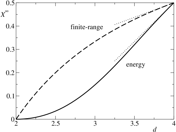
Figure 3: Asymptotic FDR $X^{\infty}$ vs dimension $d$ for finite-range observables (equation (3.3), dashed) and energy (equation (7.20), solid). Dotted lines indicate the corresponding linear expansions $1/2-\epsilon/8$ and $1/2-\epsilon/3$ in $\epsilon=4-d$.

We show in Fig. 3 the dependence of the asymptotic energy-FDR $X_{E}^{\infty}$ on dimension $d$ and compare with the result for finite-range observables. They agree in $d\geq 4$, but the difference between them grows as $d$ decreases towards $d=2$, with the energy FDR always having the lower value. In the limit $d\to 2$, both FDRs converge to zero, but while the finite-range FDR $X^{\infty}=\epsilon^{\prime}/2+{{\mathcal{O}}}(\epsilon^{\prime 2})$ does so linearly in $\epsilon^{\prime}=d-2$, the energy FDR vanishes quadratically as $X_{E}^{\infty}=\epsilon^{\prime 2}/8+{{\mathcal{O}}}(\epsilon^{\prime 3})$, due to the divergence of $\tilde{\alpha}_{d}=4/\epsilon^{\prime 2}+{{\mathcal{O}}}(1/\epsilon^{\prime})$.

As in the case $d>4$, an energy FD plot would have a pseudo-equilibrium form which hides all non-equilibrium effects at long times. Indeed, one could write (7.12) in the form $C_{E}(t,t_{\rm w})=C_{E}^{\rm eq}(t-t_{\rm w}){\mathcal{F}}_{{C_{E}}}(x)$, and the decay of the equilibrium factor $C_{E}^{\rm eq}$ squeezes all details about the aging factor ${\mathcal{F}}_{{C_{E}}}(x)$ into a vanishingly small region of the FD plot for long times. While we have not calculated ${\mathcal{F}}_{{C_{E}}}$ explicitly, the discussion after (7.12) shows that ${\mathcal{F}}_{{C_{E}}}(1)=1$ as it should be. For large $x$, on the other hand, we saw in  (7.15) that $C_{E}(t,t_{\rm w})\sim t_{\rm w}^{d/2}t^{-2}$, implying ${\mathcal{F}}_{{C_{E}}}(x)\sim t_{\rm w}^{d/2}t^{-2}(t-t_{\rm w})^{(4-d)/2}\sim x^{-d/2}$. This matches continuously at $d=4$ with the prediction (6.23) for $d>4$, where the aging correction decays as ${\mathcal{F}}_{CC}(x)\sim x^{-2}$.

8 Magnetized initial states

In this final section we consider the dynamics for initial configurations with nonzero magnetization, focussing as before on the non-equilibrium dynamics that results when the system is subsequently brought to the critical temperature $T_{\rm c}$. Physically, such a situation could arise in an “up-quench”, where the system is equilibrated at $T<T_{\rm c}$ and temperature is then increased to $T=T_{\rm c}$. As explained in the introduction, our interest in this scenario arises from recent results [20] which show that such initial conditions produce FDRs that differ nontrivially from those for zero magnetization. The analysis of [20] was limited to high dimensions $d$ or infinite-range interactions, however; the calculation below will allow us to see explicitly how the results change in finite dimension. In particular, we will obtain exact FDRs for magnetized coarsening below the upper critical dimension, i.e. $d<4$ in the spherical model.

We will continue to use the notation $C_{\mathbf{q}}(t,t_{\rm w})=(1/N)\left\langle S_{\mathbf{q}}(t)S_{\mathbf{q}}^{*}(t)\right\rangle$ for Fourier mode correlations. For $\mathbf{q}=\mathbf{0}$ this is now a full, unsubtracted correlator, with $C_{\mathbf{0}}(t,t)=Nm^{2}(t)+{{\mathcal{O}}}(1)$ and $m(t)=(1/N)\left\langle S_{\mathbf{0}}(t)\right\rangle$ the time-dependent magnetization. The difference $\tilde{C}_{\mathbf{0}}(t,t_{\rm w})=C_{\mathbf{0}}(t,t_{\rm w})-Nm(t)m(t_{\rm w})$ is the connected correlator, which has values of ${{\mathcal{O}}}(1)$ and is the relevant quantity for analysing the FD behaviour. For $\mathbf{q}\neq\mathbf{0}$, connected and full correlators coincide:

$$\tilde{C}_{\mathbf{q}}(t,t_{\rm w})=C_{\mathbf{q}}(t,t_{\rm w})-(1/N)\left\langle S_{\mathbf{q}}(t)\right\rangle\langle S^{*}_{\mathbf{q}}(t_{\rm w})\rangle=C_{\mathbf{q}}(t,t_{\rm w})$$ (8.1)

We now need to check how the analysis in the previous sections is modified by the presence of a nonzero magnetization. The Fourier space equation of motion (2.5) remains valid, and so do the resulting expressions for the response function $R_{\mathbf{q}}(t,t_{\rm w})$ (2.6) and the full correlator $C_{\mathbf{q}}(t,t_{\rm w})$ (2.10,2.13). The expression (2.16) for the Laplace transform of $g(t)$ that results from the spherical constraint also still holds, but the solution is now different. In the $\mathbf{q}$-integral, the $\mathbf{q}=\mathbf{0}$ contribution $(1/N)C_{\mathbf{0}}(0,0)/s=m^{2}(0)/s$ has to be treated separately. In fact, one sees that for $s\to 0$ this term always dominates the rest of the integral, which diverges less strongly. At criticality, where $T=T_{\rm c}=[\int(dq)\,1/\omega]^{-1}=[2\hat{f}(0)]^{-1}$, one thus has for $s\to 0$

$$2T_{\rm c}\hat{g}(s)=\frac{m^{2}(0)}{s}\left[\int(dq)\,\left(\frac{1}{2\omega}-\frac{1}{s+2\omega}\right)\right]^{-1}$$ (8.2)

which using (4.22) can be rearranged into

$$\frac{\hat{g}(s)}{m^{2}(0)}=s^{-2}\left[\int(dq)\frac{T_{\rm c}}{\omega(2\omega+s)}\right]^{-1}=[s^{2}\hat{K}_{\rm eq}(s)]^{-1}$$ (8.3)

For $d>4$, $\hat{K}_{\rm eq}(0)$ is finite so this scales as $s^{-2}$; for $d<4$, on the other hand, $\hat{K}_{\rm eq}(s)$ diverges as $s^{(d-4)/2}$ so that $\hat{g}(s)\sim s^{-d/2}$. Translating back to the time domain, $g(t)$ behaves for large $t$ as

$$g(t)\sim m^{2}(0)\,t^{\alpha},\qquad\alpha=\left\{\begin{array}[]{lll}1&\mbox{ }&(d>4)\\ (d-2)/2&\mbox{ }&(d<4)\end{array}\right.$$ (8.4)

Note that this asymptotic behaviour is independent of any details of the initial condition except for the presence of a nonzero $m(0)$; it depends on the actual value of $m(0)$ only through the prefactor $m^{2}(0)$. For the time-dependence of $m(t)$, one gets by taking an average of (2.8)

$$m(t)=R_{\mathbf{0}}(t,0)m(0)=\frac{m(0)}{\sqrt{g(t)}}$$ (8.5)

Because of the proportionality of $g(t)$ to $m^{2}(0)$ for large $t$, the asymptotic decay of $m(t)$ is independent of the initial conditions, in terms of both the decay exponent and the prefactor.

8.1 Finite-range spin observables

We first analyse the correlation and response functions for observables that relate to a number of spins that is much smaller than $N$. As for the unmagnetized case, the fluctuations of the Lagrange multiplier $z$ can then be neglected. To understand the magnetized case, it is useful to shift the spin variables by $m(t)$. We will see that the equations of motion then acquire the same form as before, so that we can directly transfer the main results from the unmagnetized case. Explicitly, we consider the following decomposition of the spin variables

$$S_{i}=m+U_{i}$$ (8.6)

where $U_{i}$ is a zero-mean variable. The equation of motion (2.4) for $S_{i}$ then gives

$$\partial_{t}m+\partial_{t}{U_{i}}=-\Omega_{ij}(m+U_{j})+\xi_{i}-z(m+U_{i})$$ (8.7)

From (8.5) and the definition (2.7), $\partial_{t}\ln m(t)=-(1/2)\partial_{t}\ln g(t)=-z(t)$, so $\partial_{t}m=-zm$. Also $\sum_{j}\Omega_{ij}=0$, giving

$$\partial_{t}{U_{i}}=-\Omega_{ij}U_{j}+\xi_{i}-zU_{i}$$ (8.8)

This is the same as the equation for $S_{i}$ in the unmagnetized case, and so one can deduce directly the solutions for the correlation functions of the $U_{i}$; these are the connected correlations $\tilde{C}$. The initial values again become unimportant for long times, allowing us to work out the scaling of the $\tilde{C}$, and then together with the response $R$ also the FDR $X$. It is clear from the description in terms of the subtracted spins $U_{i}$ that there is nothing special about the case $\mathbf{q}=\mathbf{0}$, and all results will have a smooth limit as $\mathbf{q}\to\mathbf{0}$. Because we are neglecting the fluctuations of the Lagrange multiplier $z$, this limit again has to be understood as that of a block magnetization calculated over a region much larger than the correlation length (in the time regime being considered) but much smaller than the linear system size, so that $q\gg 1/L$.

Applying (2.10), we can now write down directly the connected correlation function at equal times as

$$\tilde{C}_{\mathbf{q}}(t_{\rm w},t_{\rm w})=\tilde{C}_{\mathbf{q}}(0,0)\frac{e^{-2\omega t_{\rm w}}}{g(t_{\rm w})}+2T_{\rm c}\frac{e^{-2\omega t_{\rm w}}}{g(t_{\rm w})}\int_{0}^{t_{\rm w}}dt^{\prime}e^{2\omega t^{\prime}}g(t^{\prime})$$ (8.9)

At long times, the first term is subleading due to the scaling (8.4), and one has the behaviour

$$\tilde{C}_{\mathbf{q}}(t_{\rm w},t_{\rm w})=\frac{T_{\rm c}}{\omega}{\mathcal{F}}_{C}(\omega t_{\rm w}),\quad{\mathcal{F}}_{C}(w)=2w\int_{0}^{1}dy\,y^{\alpha}e^{-2w(1-y)}$$ (8.10)

This result is of course the same as (3.4), except for the replacement of $-\kappa$ by $\alpha$ which reflects the difference in the asymptotic behaviour of $g(t)$.

The two-time connected correlations are $\tilde{C}_{\mathbf{q}}(t,t_{\rm w})=R_{\mathbf{q}}(t,t_{\rm w})\tilde{C}_{\mathbf{q}}(t_{\rm w},t_{\rm w})$ with $R_{\mathbf{q}}(t,t_{\rm w})$ given by (2.6) as before. As a consequence, the expression (3.1) for the FDR $X_{\mathbf{q}}$ also remains valid, and one finds the scaling form $X_{\mathbf{q}}(t,t_{\rm w})={\mathcal{F}}_{X}(\omega t_{\rm w})$ with

$${\mathcal{F}}_{X}^{-1}(w)=2-(2w+\alpha)\int_{0}^{1}dy\ y^{\alpha}e^{-2w(1-y)}$$ (8.11)

which is directly analogous to (3.4). In the limit $w=\omega t_{\rm w}\rightarrow\infty$, $X_{\mathbf{q}}=1$, which means that all modes with $\mathbf{q}\neq 0$ equilibrate once $t_{\rm w}\gg 1/\omega$. In the opposite limit $w\rightarrow 0$, corresponding to $t_{\rm w}\ll 1/\omega$,

$$X_{\mathbf{q}}=\frac{\alpha+1}{\alpha+2}=\left\{\begin{array}[]{lll}2/3&\mbox{ }&(d>4)\\ d/(d+2)&\mbox{ }&(d<4)\end{array}\right.$$ (8.12)

For $\mathbf{q}\to\mathbf{0}$ this result applies independently of the value of $t_{\rm w}$ as long as $t_{\rm w}\gg 1$, so that the FDR for the block magnetization will be a straight line with slope (8.12). This is as for the unmagnetized case, but the actual value of the FDR is now different. It is also different from the value $X^{\infty}=4/5$ predicted for Ising models in the limit of large $d$ [20]; we will see below that the latter value is obtained for the global magnetization, which is affected by local spin fluctuations of ${{\mathcal{O}}}(N^{-1/2})$.

For later reference we write down the long-time forms of the correlation and response functions for $\mathbf{q}\to\mathbf{0}$. By setting $\omega=0$ in (8.9) and taking the long-time limit where the first term becomes negligible, we find for the connected equal-time correlator

$$\tilde{C}_{\mathbf{0}}(t_{\rm w},t_{\rm w})=\frac{2T_{\rm c}t_{\rm w}}{1+\alpha}$$ (8.13)

The response function is, from (2.6) and (8.5),

$$R_{\mathbf{0}}(t,t_{\rm w})=\sqrt{\frac{g(t_{\rm w})}{g(t)}}=\frac{m(t)}{m(t_{\rm w})}=\left(\frac{t_{\rm w}}{t}\right)^{\alpha/2}$$ (8.14)

where the last equality holds for long times. The two-time correlator is therefore

$$\tilde{C}_{\mathbf{0}}(t,t_{\rm w})=\frac{2T_{\rm c}t_{\rm w}}{1+\alpha}\left(\frac{t_{\rm w}}{t}\right)^{\alpha/2}$$ (8.15)

From these results one of course retrieves the long-time FDR $X_{\mathbf{0}}(t,t_{\rm w})={T_{\rm c}R_{\mathbf{0}}(t,t_{\rm w})}/{\tilde{C}_{\mathbf{0}}^{\prime}(t,t_{\rm w})}=({\alpha+1})/({\alpha+2})$, obtained in (8.12) via the limit $\omega t_{\rm w}\to 0$. As explained above, these results apply in the regime $1/L\ll q\ll 1$. For $\mathbf{q}=\mathbf{0}$ itself, they capture only the Gaussian part of the spin-fluctuations, and non-Gaussian corrections become relevant as discussed in the next section.

8.2 General expressions for magnetization correlation and response

We now turn to the FD behaviour of the global magnetization, corresponding to $\mathbf{q}=\mathbf{0}$ rather than $q\gg{1}/{L}$. All $N$ spins are now involved and one needs to account for the fluctuating contribution of the Lagrange multiplier, which we write as $z+N^{-1/2}\Delta z$ as before. To understand why this is necessary in the magnetized case, but was not in the unmagnetized scenario, consider the equation of motion (2.5) for the zero-wavevector Fourier component of the spins,

$$\partial_{t}S_{\mathbf{0}}=-(z+N^{-1/2}\Delta z)S_{\mathbf{0}}+\xi_{\mathbf{0}}$$ (8.16)

In the unmagnetized case, $S_{\mathbf{0}}$ is a zero-mean quantity of ${{\mathcal{O}}}(N^{1/2})$. The $\Delta z$-term then contributes only subleading ${{\mathcal{O}}}(1)$ fluctuations. For nonzero magnetization, on the other hand, the mean of $S_{\mathbf{0}}$ is $Nm$, with fluctuations around this of ${{\mathcal{O}}}(N^{1/2})$. The coupling of $\Delta z$ with $m$ then gives an ${{\mathcal{O}}}(N^{1/2})$ contribution to $\partial_{t}S_{\mathbf{0}}$, which is no longer negligible.

To find the resulting non-Gaussian fluctuations in $S_{\mathbf{0}}$ explicitly, we make the decomposition $S_{i}=s_{i}+N^{-1/2}r_{i}$ as before. The discussion in Sec. 4 then goes through, and we retrieve (4.11) for the ${{\mathcal{O}}}(N^{-1/2})$-corrections $r_{i}$ to the spins. For the zero Fourier mode, in particular, we have

$$r_{\mathbf{0}}(t)=-\frac{1}{2}\int dt^{\prime}dt^{\prime\prime}R_{\mathbf{0}}(t,t^{\prime})s_{\mathbf{0}}(t^{\prime})L(t^{\prime},t^{\prime\prime})\Delta(t^{\prime\prime})$$ (8.17)

To simplify the calculation of connected correlations, we now decompose the Gaussian part of the spins into $s_{i}=m+u_{i}$, so that the $u_{i}$ are zero-mean Gaussian variables. This corresponds to a decomposition $U_{i}=u_{i}+\sqrt{N}r_{i}$ of the fluctuating parts of the spins into leading Gaussian terms and small non-Gaussian corrections, in analogy to the representation $S_{i}=s_{i}+\sqrt{N}r_{i}$ in the unmagnetized case. The $u_{i}$ obey the equation of motion (8.8), and their correlation and response functions are the $\tilde{C}_{\mathbf{q}}$ and $R_{\mathbf{q}}$ calculated previously.

We will write the connected correlation function for the global magnetization which includes non-Gaussian corrections as $C_{\rm m}(t,t_{\rm w})=(1/N)\left\langle U_{\mathbf{0}}(t)U_{\mathbf{0}}(t_{\rm w})\right\rangle$. Making the decomposition into Gaussian and non-Gaussian parts, this reads

$$C_{\rm m}(t,t_{\rm w})=\frac{1}{N}\langle[u_{\mathbf{0}}(t)+N^{-1/2}r_{\mathbf{0}}(t)][u_{\mathbf{0}}(t_{\rm w})+N^{-1/2}r_{\mathbf{0}}(t_{\rm w})]\rangle$$ (8.18)

with, from (8.17),

$$r_{\mathbf{0}}(t) = -\frac{1}{2}\int dt^{\prime}\,dt^{\prime\prime}\,R_{\mathbf{0}}(t,t^{\prime})[Nm(t^{\prime})+u_{\mathbf{0}}(t^{\prime})]L(t^{\prime},t^{\prime\prime})\Delta(t^{\prime\prime})$$ (8.19)

$$= -\frac{N}{2}\int dt^{\prime}\,M(t,t^{\prime})\Delta(t^{\prime})$$ (8.20)

Here we have defined

$$M(t,t_{\rm w})=\int dt^{\prime}\,R_{\mathbf{0}}(t,t^{\prime})m(t^{\prime})L(t^{\prime},t_{\rm w})=m(t)\int^{t}dt^{\prime}\,L(t^{\prime},t_{\rm w})$$ (8.21)

where the second form follows from (8.14). $M$ is, like $R$ and $L$, causal and so vanishes for $t<t_{\rm w}$. In (8.20) we have also discarded the Gaussian fluctuation term $u_{\mathbf{0}}$, which is of ${{\mathcal{O}}}(N^{1/2})$ and so negligible against the term $Nm$. This is in line with the intuition discussed earlier that non-Gaussian fluctuations arise only from the coupling of $\Delta z$ to $m$. Note also that $r_{\mathbf{0}}$ is ${{\mathcal{O}}}(N)$, so that in (8.18) the non-Gaussian correction $N^{-1/2}r_{\mathbf{0}}$ is of the same order as the Gaussian fluctuation $u_{\mathbf{0}}$, again as expected.

Substituting (8.20) into (8.18), we see that we need the two-time correlations of $u_{\mathbf{0}}$ and $\Delta$. In the presence of a nonzero $m$ the latter becomes

$$\Delta=\frac{1}{\sqrt{N}}\sum_{i}(s_{i}^{2}-1)=\frac{1}{\sqrt{N}}\sum_{i}(m^{2}-1+2u_{i}m+u_{i}^{2})$$ (8.22)

The required correlations are therefore $\left\langle u_{\mathbf{0}}(t)u_{\mathbf{0}}(t_{\rm w})\right\rangle=N\tilde{C}_{\mathbf{0}}(t,t_{\rm w})$ and

$$\langle u_{\mathbf{0}}(t)\Delta(t^{\prime})\rangle = \frac{1}{\sqrt{N}}\sum_{ij}\langle u_{i}(t)[m^{2}(t^{\prime})-1+2u_{j}(t^{\prime})m(t^{\prime})+u_{j}^{2}(t^{\prime})]\rangle$$ (8.23)

$$= \frac{2}{\sqrt{N}}m(t^{\prime})\sum_{ij}\langle u_{i}(t)u_{j}(t^{\prime})\rangle=2m(t^{\prime})\sqrt{N}\tilde{C}_{\mathbf{0}}(t,t^{\prime})$$ (8.24)

For the autocorrelation of $\Delta$, we can exploit the fact that $\left\langle\Delta\right\rangle=0$ to write (8.22) as $\Delta=N^{-1/2}\sum_{i}(2u_{i}m+u_{i}^{2}-\left\langle u_{i}^{2}\right\rangle)$. This gives

$$\langle\Delta(t^{\prime})\Delta(t_{\rm w}^{\prime})\rangle = \frac{1}{N}\sum_{ik}\langle[2u_{i}(t^{\prime})m(t^{\prime})+u_{i}^{2}(t^{\prime})-\langle u_{i}^{2}(t^{\prime})\rangle][\cdots t^{\prime}\rightarrow t_{\rm w}^{\prime}\cdots]\rangle$$ (8.25)

$$= \frac{4}{N}m(t^{\prime})m(t_{\rm w}^{\prime})\sum_{ij}\langle u_{i}(t^{\prime})u_{j}(t_{\rm w}^{\prime})\rangle+\frac{2}{N}\sum_{ij}\langle u_{i}(t^{\prime})u_{j}(t_{\rm w}^{\prime})\rangle^{2}$$ (8.26)

$$= 4m(t^{\prime})m(t_{\rm w}^{\prime})\tilde{C}_{\mathbf{0}}(t^{\prime},t_{\rm w}^{\prime})+2\int(dq)\,\tilde{C}_{\mathbf{q}}^{2}(t^{\prime},t_{\rm w}^{\prime})$$ (8.27)

where we have used Wick’s theorem to simplify the fourth-order average $\langle(u_{i}^{2}-\langle u_{i}^{2}\rangle)(u_{j}^{2}-\langle u_{j}^{2}\rangle)\rangle=\langle u_{i}^{2}u_{j}^{2}\rangle-\langle u_{i}^{2}\rangle\langle u_{j}^{2}\rangle=2\langle u_{i}u_{j}\rangle^{2}$. Abbreviating the $q$-integral as $\tilde{C}\tilde{C}(t^{\prime},t_{\rm w}^{\prime})$, the full connected correlation function (8.18) can thus be written as

$$C_{\rm m}(t,t_{\rm w}) = \tilde{C}_{\mathbf{0}}(t,t_{\rm w})-\frac{1}{2\sqrt{N}}\int dt^{\prime}\,M(t,t^{\prime})\langle u_{\mathbf{0}}(t_{\rm w})\Delta(t^{\prime})\rangle$$ (8.28)

$${}-{}\frac{1}{2\sqrt{N}}\int dt^{\prime}\,M(t_{\rm w},t^{\prime})\langle u_{\mathbf{0}}(t)\Delta(t^{\prime})\rangle$$

$${}+{}\frac{1}{4}\int\,dt^{\prime}\,dt_{\rm w}^{\prime}\,M(t,t^{\prime})M(t_{\rm w},t_{\rm w}^{\prime})\langle\Delta(t_{\rm w}^{\prime})\Delta(t^{\prime})\rangle$$

$$= C_{\rm m}^{(1)}(t,t_{\rm w})+C_{\rm m}^{(2)}(t,t_{\rm w})$$ (8.29)

where

$$C_{\rm m}^{(1)}(t,t_{\rm w}) = \tilde{C}_{\mathbf{0}}(t,t_{\rm w})-\int dt^{\prime}\,[M(t,t^{\prime})\tilde{C}_{\mathbf{0}}(t_{\rm w},t^{\prime})+M(t_{\rm w},t^{\prime})\tilde{C}_{\mathbf{0}}(t,t^{\prime})]m(t^{\prime})$$ (8.31)

$${}+{}\int\,dt^{\prime}\,dt_{\rm w}^{\prime}\,M(t,t^{\prime})M(t_{\rm w},t_{\rm w}^{\prime})m(t^{\prime})m(t_{\rm w}^{\prime})\tilde{C}_{\mathbf{0}}(t^{\prime},t_{\rm w}^{\prime})$$

$$= \int\,dt^{\prime}\,dt_{\rm w}^{\prime}\,[\delta(t-t^{\prime})-M(t,t^{\prime})m(t^{\prime})]$$

$$\times[\delta(t_{\rm w}-t_{\rm w}^{\prime})-M(t_{\rm w},t_{\rm w}^{\prime})m(t_{\rm w}^{\prime})]\tilde{C}_{\mathbf{0}}(t^{\prime},t_{\rm w}^{\prime})$$

and

$$C_{\rm m}^{(2)}(t,t_{\rm w})=\frac{1}{2}\int\,dt^{\prime}\,dt_{\rm w}^{\prime}\,M(t,t^{\prime})M(t_{\rm w},t_{\rm w}^{\prime})\tilde{C}\tilde{C}(t^{\prime},t_{\rm w}^{\prime})$$ (8.32)

Next we derive an expression for the corresponding magnetization response function. To this purpose we expand the spins for small fields as

$$S_{i}=s_{i}+hr_{i}$$ (8.33)

where $s_{i}$ are the unperturbed spins and we neglect the ${{\mathcal{O}}}(N^{-1/2})$ non-Gaussian corrections as irrelevant, as in the unmagnetized case. The Lagrange multiplier is similarly written as $z+h\Delta z$. By collecting the ${{\mathcal{O}}}(h)$ terms from the equation of motion for the $S_{i}$, we then find by analogy with (5.21) that the $r_{i}$ obey

$$\partial_{t}{r_{i}}=-\Omega_{ij}r_{j}-zr_{i}-\Delta z\,s_{i}+\delta(t-t_{\rm w})$$ (8.34)

Here the last term represents a field impulse at time $t_{\rm w}$, uniform over all sites as is appropriate for the field conjugate to the global magnetization. Since $r_{i}(t)=0$ before the field is applied, i.e. for $t<t_{\rm w}$, this impulse perturbation gives $r_{i}(t_{\rm w}^{+})=1$. Starting from this value we can then integrate (8.34) forward in time to get

$$r_{i}(t)=\sum_{j}R_{ij}(t,t_{\rm w})-\int_{t_{\rm w}}^{t}dt^{\prime}\,R_{ij}(t,t^{\prime})\Delta z(t^{\prime})s_{j}(t^{\prime})$$ (8.35)

The condition we need to impose in order to get $\Delta z$ is that the spherical constraint $(1/N)\sum_{i}(s_{i}+hr_{i})^{2}=1$ needs to be satisfied to linear order in $h$, giving the condition $({1}/{N})\sum_{i}\langle r_{i}s_{i}\rangle=0$. Inserting (8.35) into this yields

$$R_{\mathbf{0}}(t,t_{\rm w})m(t)=\int_{t_{\rm w}}^{t}dt^{\prime}\,K(t,t^{\prime})\Delta z(t^{\prime})$$ (8.36)

where we have used the definition (4.8) of $K(t,t^{\prime})$. Applying the inverse kernel $L$ gives

$$\Delta z(t)=\int_{t_{\rm w}}^{t}dt^{\prime}\,L(t,t^{\prime})m(t^{\prime})R_{\mathbf{0}}(t^{\prime},t_{\rm w})$$ (8.37)

Note that this result vanishes when $m=0$, consistent with the fact that we did not need to consider perturbations of $z$ in our calculation of the magnetization response in the unmagnetized case. We can now write down the magnetization response function, which we denote by $R_{\rm m}(t,t_{\rm w})$. It is given by $R_{\rm m}=({1}/{N})\sum_{i}\langle r_{i}\rangle$; inserting the result for $\Delta z$ into (8.35), we get explicitly

$$R_{\rm m}(t,t_{\rm w}) = R_{\mathbf{0}}(t,t_{\rm w})-\int dt^{\prime\prime}\,dt^{\prime}\,R_{\mathbf{0}}(t,t^{\prime\prime})m(t^{\prime\prime})L(t^{\prime\prime},t^{\prime})m(t^{\prime})R_{\mathbf{0}}(t^{\prime},t_{\rm w})$$ (8.38)

$$= \int dt^{\prime}\,[\delta(t-t^{\prime})-M(t,t^{\prime})m(t^{\prime})]R_{\mathbf{0}}(t^{\prime},t_{\rm w})$$ (8.39)

This completes the derivation of the general expressions for the magnetization correlation and response. To make progress, we need to find the kernel $M(t,t^{\prime})$. This requires $L(t,t^{\prime})$, which is the inverse of $K(t,t^{\prime})=\int(dq)\,R_{\mathbf{q}}(t,t^{\prime})C_{\mathbf{q}}(t,t^{\prime})$. As is clear from the discussion in Sec. 4, the correlator occurring here is the unsubtracted one. Because $C_{\mathbf{0}}(t,t^{\prime})=Nm(t)m(t^{\prime})$ is ${{\mathcal{O}}}(N)$, the $\mathbf{q}=\mathbf{0}$ term needs to be treated separately in spite of its vanishing weight $1/N$. It makes a contribution $(1/N)R_{\mathbf{0}}(t,t^{\prime})Nm(t)m(t^{\prime})=m^{2}(t)\theta(t-t^{\prime})$, where we have simplified using (8.14). We can thus write

$$K(t,t^{\prime})=\tilde{K}(t,t^{\prime})+m^{2}(t)\theta(t-t^{\prime})$$ (8.40)

with the $\mathbf{q}\neq\mathbf{0}$ contribution

$$\tilde{K}(t,t^{\prime})=\int(dq)\,R_{\mathbf{q}}(t,t^{\prime})\tilde{C}_{\mathbf{q}}(t,t^{\prime})$$ (8.41)

We have switched to the connected correlator here; this makes no difference for $\mathbf{q}\neq 0$, but allows us to include $\mathbf{q}=\mathbf{0}$ in the integral because $\tilde{C}_{\mathbf{0}}={{\mathcal{O}}}(1)$. To say more, we will need to distinguish between dimensions $d>4$ and $d<4$.

8.3 Magnetization correlation and response: Non-equilibrium, $d>4$

The scaling of the connected part $\tilde{K}$ of $K$ can be analysed exactly as in the case of zero magnetization: it consists of the same equilibrium time dependence modulated by an aging function, $\tilde{K}(t,t^{\prime})=K_{\rm eq}(t-t^{\prime}){\mathcal{F}}_{\tilde{K}}(t/t^{\prime})$. The aging part can be worked out exactly as in (4.15) with the only difference arising from the changed asymptotic behaviour of $g(t)\sim t^{\alpha}$ rather than $t^{-\kappa}$. For ${\mathcal{F}}_{\tilde{K}}$ we can therefore use directly (4.16), with $\kappa$ replaced by $-\alpha$:

$${\mathcal{F}}_{\tilde{K}}(x) = \frac{d-2}{2}(x-1)^{(d-2)/2}x^{-\alpha}\int_{0}^{1}dy\,y^{\alpha}(x-y)^{-d/2}$$ (8.42)

In $d>4$, where $\alpha=1$, the integral can be computed explicitly to give

$${\mathcal{F}}_{\tilde{K}}(x)=1-\frac{d-2}{d-4}\left(\frac{x-1}{x}\right)+\frac{2}{d-4}\left(\frac{x-1}{x}\right)^{\frac{d-2}{2}}$$ (8.43)

We will see below that the precise behaviour of this function does not affect the results. Briefly though, for $x-1\ll 1$ the second term on the r.h.s. is leading so that ${\mathcal{F}}_{\tilde{K}}$ decreases linearly with $x-1$, while for large $x$ one finds by expanding in $1/x$ that ${\mathcal{F}}_{\tilde{K}}\approx[(d-2)/4]x^{-2}$.

To find the inverse kernel $L$, consider how $K(t,t^{\prime})$ varies with $t$. The first part in (8.40) starts off close to unity and decays on ${{\mathcal{O}}}(1)$ timescales $t-t^{\prime}$ as $K_{\rm eq}(t-t^{\prime})$, with a modulation by the aging factor ${\mathcal{F}}_{\tilde{K}}(t/t^{\prime})$ once $t-t^{\prime}$ becomes comparable to $t^{\prime}$. The second part, on the other hand, is small initially but only decays on aging timescales. Comparing $K_{\rm eq}(t-t^{\prime})\sim(t-t^{\prime})^{(2-d)/2}$ to $m^{2}(t)\sim 1/t$, this second term therefore eventually becomes dominant, for $t-t^{\prime}\sim t^{2/(d-2)}$. This discussion suggests that also the inverse kernel $L$ should be composed of two parts with distinct long-time behaviour. We therefore write

$$L=\tilde{L}+L_{\mathbf{0}}$$ (8.44)

where $\tilde{L}$ is the inverse of $\tilde{K}$ and $L_{\mathbf{0}}$ arises from the zero-wavevector part of $K$. The continuous part of $L$ is then similarly decomposed as $L^{(2)}=\tilde{L}^{(2)}+L^{(2)}_{\mathbf{0}}$.

We proceed by writing the defining equations for $L^{(2)}$ and $\tilde{L}^{(2)}$. The full inverse $L$ is defined by (4.9) and as before has singular parts which are related to the behaviour of $K(t,t^{\prime})$ for $t\to t^{\prime}$. One can show directly from the definition of $K$, and exactly as in the unmagnetized case, that

$$K(t^{\prime+},t^{\prime})=1,\qquad\left.\partial_{t^{\prime}}K(t,t^{\prime})\right|_{t\to t^{\prime+}}=2T_{\rm c}$$ (8.45)

The decomposition (4.12) of the inverse kernel $L$ therefore also remains valid, and from (4.9) and (8.40) we get the following equation for its continuous part $L^{(2)}$

$$\int dt^{\prime}\,[\tilde{K}(t,t^{\prime})+m^{2}(t)]L^{(2)}(t^{\prime},t_{\rm w})=2T_{\rm c}\tilde{K}(t,t_{\rm w})+2T_{\rm c}m^{2}(t)-\partial_{t_{\rm w}}\tilde{K}(t,t_{\rm w})$$ (8.46)

This is the analogue of the relation (4.19) for the case $m=0$. We can argue similarly for $\tilde{L}$, which is defined by

$$\int dt^{\prime}\,\tilde{K}(t,t^{\prime})\tilde{L}(t^{\prime},t_{\rm w})=\delta(t-t_{\rm w})$$ (8.47)

From (8.40) and (8.45),

$$\tilde{K}(t^{\prime+},t^{\prime})=1-m^{2}(t),\qquad\left.\partial_{t^{\prime}}\tilde{K}(t,t^{\prime})\right|_{t\to t^{\prime+}}=2T_{\rm c}$$ (8.48)

and this initial behaviour implies that $\tilde{L}$ can be decomposed as

$$\tilde{L}(t^{\prime},t_{\rm w})=\frac{\delta^{\prime}(t^{\prime}-t_{\rm w})}{1-m^{2}(t_{\rm w})}+\frac{2T_{\rm c}}{[1-m^{2}(t_{\rm w})]^{2}}\delta(t^{\prime}-t_{\rm w})-\tilde{L}^{(2)}(t^{\prime},t_{\rm w})$$ (8.49)

Inserting into the definition (8.47) gives for the continuous part $\tilde{L}^{(2)}$

$$\int dt^{\prime}\,\tilde{K}(t,t^{\prime})\tilde{L}^{(2)}(t^{\prime},t_{\rm w})=\frac{2T_{\rm c}}{[1-m^{2}(t_{\rm w})]^{2}}\tilde{K}(t,t_{\rm w})-\frac{1}{1-m^{2}(t_{\rm w})}\partial_{t_{\rm w}}\tilde{K}(t,t_{\rm w})$$ (8.50)

Now for long times, we can approximate $1-m^{2}(t_{\rm w})\approx 1$. Then (8.50) becomes identical to the relation (4.19) which determined $L^{(2)}$ in the unmagnetized case. Since $\tilde{K}$ has the same scaling form as $K$ in (4.19), except for the replacement of ${\mathcal{F}}_{K}$ by ${\mathcal{F}}_{\tilde{K}}$, the solution for $\tilde{L}^{(2)}$ can be found in exactly the same way. In particular, the scaling functions describing the aging corrections in $\tilde{K}$ and $\tilde{L}^{(2)}$ are again identical, and we can write directly

$$\tilde{L}^{(2)}(t,t^{\prime})=L^{(2)}_{\rm eq}(t-t^{\prime}){\mathcal{F}}_{\tilde{K}}(t/t^{\prime})$$ (8.51)

as the long-time form of $\tilde{L}^{(2)}$. Here $L^{(2)}_{\rm eq}$ is the same function as in the unmagnetized case, with Laplace transform (4.21).

It now remains to find $L^{(2)}_{\mathbf{0}}$. Subtracting (8.50) from (8.46) gives

$$\int_{t_{\rm w}}^{t}dt^{\prime}\,\tilde{K}(t,t^{\prime})L^{(2)}_{\mathbf{0}}(t^{\prime},t_{\rm w})+m^{2}(t)\int_{t_{\rm w}}^{t}dt^{\prime}\,L^{(2)}_{\mathbf{0}}(t^{\prime},t_{\rm w})=2T_{\rm c}\frac{-2m^{2}(t_{\rm w})+m^{4}(t_{\rm w})}{[1-m^{2}(t_{\rm w})]^{2}}\tilde{K}(t,t_{\rm w})$$ (8.52)

$${}+{}m^{2}(t)\left[2T_{\rm c}-\int_{t_{\rm w}}^{t}dt^{\prime}\,\tilde{L}^{(2)}(t^{\prime},t_{\rm w})\right]+\frac{m^{2}(t_{\rm w})}{1-m^{2}(t_{\rm w})}\partial_{t_{\rm w}}\tilde{K}(t,t_{\rm w})$$

To make progress we assume that, by analogy with the structure (8.40) of $K$, $L^{(2)}_{\mathbf{0}}$ varies only on aging timescales; we will find this confirmed a posteriori. We can then concentrate on the aging regime $t-t_{\rm w}\sim t_{\rm w}\gg 1$. In this regime, the integral $\int_{t_{\rm w}}^{t}dt^{\prime}\,\tilde{L}^{(2)}(t^{\prime},t_{\rm w})=\int_{t_{\rm w}}^{t}dt^{\prime}\,L^{(2)}_{\rm eq}(t^{\prime}-t_{\rm w}){\mathcal{F}}_{\tilde{K}}(t^{\prime}/t_{\rm w})$ on the r.h.s. of (8.52) becomes to leading order $\int_{t_{\rm w}}^{\infty}dt^{\prime}\,L^{(2)}_{\rm eq}(t^{\prime}-t_{\rm w})=\hat{L}^{(2)}_{\rm eq}(0)$; the aging correction ${\mathcal{F}}_{\tilde{K}}$ is unimportant because the integral converges for $t^{\prime}-t_{\rm w}={{\mathcal{O}}}(1)$, and the upper integration limit can be set to infinity for the same reason. From (4.21), $\hat{L}^{(2)}_{\rm eq}(0)=2T_{\rm c}-1/\hat{K}_{\rm eq}(0)$, and so the square bracket on the r.h.s. of (8.52) becomes simply the constant $1/\hat{K}_{\rm eq}(0)$. In the first and third term on the r.h.s., on the other hand, $\tilde{K}$ and $\partial_{t_{\rm w}}\tilde{K}$ scale as $(t-t_{\rm w})^{-(d-2)/2}$ and $(t-t_{\rm w})^{-d/2}$, respectively, and are negligible compared to the second term in the aging regime. Disregarding these subleading terms, equation (8.52) is transformed to

$$\int_{t_{\rm w}}^{t}dt^{\prime}\,\tilde{K}(t,t^{\prime})L^{(2)}_{\mathbf{0}}(t^{\prime},t_{\rm w})+m^{2}(t)\int_{t_{\rm w}}^{t}dt^{\prime}\,L^{(2)}_{\mathbf{0}}(t^{\prime},t_{\rm w})=\frac{m^{2}(t)}{\hat{K}_{\rm eq}(0)}$$ (8.53)

In the first integral, if as assumed $L^{(2)}_{\mathbf{0}}$ varies only on aging timescales, the integral is dominated by the region $t^{\prime}\approx t$ because of the factor $K_{\rm eq}(t-t^{\prime})$ in $\tilde{K}(t,t^{\prime})$. This factor again makes the integral convergent within a region $t-t^{\prime}={{\mathcal{O}}}(1)$, and so we can approximate it by $\hat{K}_{\rm eq}(0)L^{(2)}_{\mathbf{0}}(t,t_{\rm w})$. This gives

$$\int_{t_{\rm w}}^{t}dt^{\prime}\,L^{(2)}_{\mathbf{0}}(t^{\prime},t_{\rm w})=\frac{1}{\hat{K}_{\rm eq}(0)}-\frac{\hat{K}_{\rm eq}(0)}{m^{2}(t)}L^{(2)}_{\mathbf{0}}(t,t_{\rm w})$$ (8.54)

and specifically in the limit $t/t_{\rm w}\to 1$

$$L^{(2)}_{\mathbf{0}}(t_{\rm w},t_{\rm w})=\hat{K}_{\rm eq}^{-2}(0)m^{2}(t_{\rm w})$$ (8.55)

To find $L^{(2)}_{\mathbf{0}}$ for $t/t_{\rm w}>1$, we use that $m^{2}(t)=\mu_{d}/t$ for large $t$ and in $d>4$, see (8.4,8.5), with some dimension-dependent coefficient $\mu_{d}$. Taking a derivative of (8.54) with respect to $t$ then gives

$$L^{(2)}_{\mathbf{0}}(t,t_{\rm w})\left[1+\mu_{d}^{-1}\hat{K}_{\rm eq}(0)\right]=-t{\mu_{d}}^{-1}\hat{K}_{\rm eq}(0)\partial_{t}L^{(2)}_{\mathbf{0}}(t,t_{\rm w})$$ (8.56)

This implies $\partial(\ln L^{(2)}_{\mathbf{0}})/\partial(\ln t)=-[1+\mu_{d}/\hat{K}_{\rm eq}(0)]$ and so together with (8.55)

$$L^{(2)}_{\mathbf{0}}(t,t_{\rm w})=\hat{K}_{\rm eq}^{-2}(0)\frac{\mu_{d}}{t_{\rm w}}\left(\frac{t}{t_{\rm w}}\right)^{-[1+\mu_{d}/\hat{K}_{\rm eq}(0)]}$$ (8.57)

This can be simplified because in fact $\mu_{d}=\hat{K}_{\rm eq}(0)$. To see this, note from (8.3) that $\hat{g}(s)/m^{2}(0)=1/[\hat{K}_{\rm eq}(0)s^{2}]$ for small $s$; here we have used that $\hat{K}_{\rm eq}(0)$ is finite for $d>4$. Transforming back to the time domain gives $g(t)/m^{2}(0)=m^{-2}(t)=t/\hat{K}_{\rm eq}(0)$ for large $t$, i.e. $m^{2}(t)=\hat{K}_{\rm eq}(0)/t$. Thus (8.57) simplifies to

$$L^{(2)}_{\mathbf{0}}(t,t_{\rm w})=\frac{t_{\rm w}}{\mu_{d}t^{2}}$$ (8.58)

This result is consistent with our assumption that $L^{(2)}_{\mathbf{0}}$ only varies on aging timescales. Overall, we have thus found for $L^{(2)}(t,t_{\rm w})$ the following long-time form

$$L^{(2)}(t,t_{\rm w})=L^{(2)}_{\rm eq}(t-t_{\rm w}){\mathcal{F}}_{\tilde{K}}\left({t}/{t_{\rm w}}\right)+\frac{t_{\rm w}}{\mu_{d}t^{2}}$$ (8.59)

Of course, for time differences $t-t_{\rm w}={{\mathcal{O}}}(1)$, $L^{(2)}_{\mathbf{0}}(t,t_{\rm w})$ will deviate from the form (8.58) derived for the aging regime. However, one can verify by expanding both sides of (8.52) to ${{\mathcal{O}}}(t-t_{\rm w})$ that, even for $t=t_{\rm w}$, $L^{(2)}_{\mathbf{0}}$ remains of order $1/t_{\rm w}$, so that these small deviations are always negligible compared to the first term in (8.59).

We can now proceed to find $M$ as defined in (8.21), and from there finally the explicit forms of the magnetization correlation and response functions. Using the general structure (4.12) of $L$ we have

$$m^{-1}(t)M(t,t_{\rm w})=\delta(t-t_{\rm w})+2T_{\rm c}-\int_{t_{\rm w}}^{t}dt^{\prime}\,L^{(2)}(t^{\prime},t_{\rm w})$$ (8.60)

The integral can be separated into the contributions from the two parts of $L^{(2)}$ as given in (8.59). The first part yields an integral that converges for $t^{\prime}-t_{\rm w}={{\mathcal{O}}}(1)$; for $t-t_{\rm w}\gg 1$, it therefore gives $\hat{L}_{\rm eq}(0)=2T_{\rm c}-1/\hat{K}_{\rm eq}(0)=2T_{\rm c}-1/\mu_{d}$ to leading order. The second part, on the other hand, yields explicitly $\int_{t_{\rm w}}^{t}dt^{\prime}(t_{\rm w}/\mu_{d}t^{\prime 2})=\mu_{d}^{-1}(1-t_{\rm w}/t)$, so that

$$m^{-1}(t)M(t,t_{\rm w})=\delta(t-t_{\rm w})+\frac{1}{\mu_{d}}-\frac{1}{\mu_{d}}\left(1-\frac{t_{\rm w}}{t}\right)=\delta(t-t_{\rm w})+\frac{1}{\mu_{d}}\frac{t_{\rm w}}{t}$$ (8.61)

This result applies for $t-t_{\rm w}\gg 1$. For $t-t_{\rm w}={{\mathcal{O}}}(1)$ it is not accurate; e.g. at $t=t_{\rm w}$ the continuous part of $m^{-1}(t)M(t,t_{\rm w})$ is, from (8.60), $2T_{\rm c}$ rather than $1/\mu_{d}$. However, this deviation over an ${{\mathcal{O}}}(1)$ time-range only gives subleading corrections in the integrals over $M$ that we need below, as indeed does the $\delta(t-t_{\rm w})$-term. This can be seen in (8.31) and (8.39), where only the combination $\delta(t-t_{\rm w})-M(t,t_{\rm w})m(t_{\rm w})$ occurs; the latter can be written as

$$\delta(t-t_{\rm w})-M(t,t_{\rm w})m(t_{\rm w})=\delta(t-t_{\rm w})[1-m(t)m(t_{\rm w})]-\frac{t_{\rm w}^{1/2}}{t^{3/2}}=\delta(t-t_{\rm w})-\frac{t_{\rm w}^{1/2}}{t^{3/2}}$$ (8.62)

The second form holds for long times, where the $m(t)m(t_{\rm w})$ term that originated from the $\delta$-term in (8.61) is negligible.

We can now work out the expression (8.29) for the full connected correlation function. One can show that the contribution $C_{\rm m}^{(2)}$ involving $\tilde{C}\tilde{C}$ is negligible in the long-time limit. In the expression (8.31) for the remainder $C_{\rm m}^{(1)}$, let us call the second and third term $I_{2}$ and $I_{3}$. We need $\tilde{C}_{\mathbf{0}}$, which from (8.15) reads $\tilde{C}_{\mathbf{0}}(t^{\prime},t_{\rm w}^{\prime})=T_{\rm c}t_{\rm w}^{\prime 3/2}t^{\prime-1/2}$ for $t^{\prime}>t_{\rm w}^{\prime}$; because $\tilde{C}_{\mathbf{0}}$ is symmetric in time this then implies $\tilde{C}_{\mathbf{0}}(t^{\prime},t_{\rm w}^{\prime})=T_{\rm c}t^{\prime 3/2}t_{\rm w}^{\prime-1/2}$ for $t^{\prime}<t_{\rm w}^{\prime}$. Paying due attention to this temporal ordering of the arguments of $\tilde{C}_{\mathbf{0}}$ and using (8.62), one finds

$$I_{2}(t,t_{\rm w}) = T_{\rm c}\left[\int_{0}^{t_{\rm w}}dt^{\prime}\,\frac{t^{\prime 1/2}}{t^{3/2}}\frac{t^{\prime 3/2}}{t_{\rm w}^{1/2}}+\int_{t_{\rm w}}^{t}dt^{\prime}\,\frac{t^{\prime 1/2}}{t^{3/2}}\frac{t_{\rm w}^{3/2}}{t^{\prime 1/2}}\right]+T_{\rm c}\int_{0}^{t_{\rm w}}dt^{\prime}\,\frac{t^{\prime 1/2}}{t_{\rm w}^{3/2}}\frac{t^{\prime 3/2}}{t^{1/2}}$$ (8.63)

$$= T_{\rm c}\left(\frac{t_{\rm w}}{t}\right)^{3/2}\left(\frac{4}{3}t-\frac{2}{3}t_{\rm w}\right)$$ (8.64)

Similarly, the double integral in (8.31) can be evaluated as

$$I_{3}(t,t_{\rm w}) = \int_{0}^{t}dt^{\prime}\int_{0}^{t_{\rm w}}\!\!dt_{\rm w}^{\prime}\,\frac{t^{\prime 1/2}}{t^{3/2}}\frac{t_{\rm w}^{\prime 1/2}}{t_{\rm w}^{3/2}}\,\tilde{C}_{\mathbf{0}}(t_{\rm w}^{\prime},t^{\prime})$$ (8.65)

$$= T_{\rm c}\int_{t_{\rm w}}^{t}dt^{\prime}\int_{0}^{t_{\rm w}}\!\!dt_{\rm w}^{\prime}\,\frac{t^{\prime 1/2}}{t^{3/2}}\frac{t_{\rm w}^{\prime 1/2}}{t_{\rm w}^{3/2}}\frac{t_{\rm w}^{\prime 3/2}}{t^{\prime 1/2}}+2T_{\rm c}\int_{0}^{t_{\rm w}}\!\!dt^{\prime}\int_{0}^{t^{\prime}}\!\!dt_{\rm w}^{\prime}\,\frac{t^{\prime 1/2}}{t^{3/2}}\frac{t_{\rm w}^{\prime 1/2}}{t_{\rm w}^{3/2}}\frac{t_{\rm w}^{\prime 3/2}}{t^{\prime 1/2}}$$ (8.66)

$$= \frac{T_{\rm c}}{3}\left(\frac{t_{\rm w}}{t}\right)^{3/2}(t-t_{\rm w})+\frac{2T_{\rm c}}{3}\int_{0}^{t_{\rm w}}dt^{\prime}\frac{t^{\prime 3}}{t^{3/2}t_{\rm w}^{3/2}}$$ (8.67)

$$= \frac{T_{\rm c}}{6}\left(\frac{t_{\rm w}}{t}\right)^{3/2}(2t-t_{\rm w})$$ (8.68)

Our final long-time result for the connected magnetization correlator including non-Gaussian corrections is then

$$C_{\rm m}(t,t_{\rm w}) = T_{\rm c}\frac{t_{\rm w}^{3/2}}{t^{1/2}}+I_{2}(t,t_{\rm w})+I_{3}(t,t_{\rm w})$$ (8.69)

$$= T_{\rm c}\left(\frac{t_{\rm w}}{t}\right)^{3/2}\left(t-\frac{4}{3}t+\frac{2}{3}t_{\rm w}+\frac{1}{3}t-\frac{1}{6}t_{\rm w}\right)\ =\ \frac{T_{\rm c}t_{\rm w}}{2}\left(\frac{t_{\rm w}}{t}\right)^{3/2}$$ (8.70)

For the conjugate magnetization response function we get from (8.39) and (8.61), together with $R_{\mathbf{0}}(t,t_{\rm w})=(t_{\rm w}/t)^{1/2}$,

$$R_{\rm m}(t,t_{\rm w}) = R_{\mathbf{0}}(t,t_{\rm w})-\int_{t_{\rm w}}^{t}dt^{\prime}\,\frac{t^{\prime 1/2}}{t^{3/2}}R_{\mathbf{0}}(t^{\prime},t_{\rm w})$$ (8.71)

$$= \left(\frac{t_{\rm w}}{t}\right)^{1/2}-\frac{t_{\rm w}^{1/2}}{t^{3/2}}(t-t_{\rm w})=\left(\frac{t_{\rm w}}{t}\right)^{3/2}$$ (8.72)

The FDR follows finally as

$$X_{\rm m}(t,t_{\rm w})=\frac{T_{\rm c}R_{\rm m}(t,t_{\rm w})}{C_{\rm m}^{\prime}(t,t_{\rm w})}=\frac{4}{5}$$ (8.73)

Interestingly, this agrees exactly with the result for the Ising ferromagnet in the limit of large dimensionality $d$ [20]. As in the unmagnetized case, we see therefore that it is the global observables in the spherical model, which are strongly affected by non-Gaussian fluctuations, that behave like their analogues in short-range models. In fact, even the expressions for the correlation and response functions we find here are identical to those in the large-$d$ Ising case, implying “universality” at a more detailed level than one might have expected.

It is worth noting that the effect of the non-Gaussian corrections is very large: compared to the Gaussian result $\tilde{C}_{\mathbf{0}}(t,t_{\rm w})\sim t_{\rm w}(t_{\rm w}/t)^{1/2}$, the corrections increase the decay exponent to $C_{\rm m}(t,t_{\rm w})\sim t_{\rm w}(t_{\rm w}/t)^{3/2}$, so that $C_{\rm m}/\tilde{C}_{\mathbf{0}}\sim t_{\rm w}/t\ll 1$ for $t\gg t_{\rm w}$: there is an almost perfect cancellation of Gaussian terms and non-Gaussian corrections for well-separated times. Similar comments apply to the response. The overall effect of the non-Gaussian corrections on the FD relation is to leave this as a straight line (since $X$ is constant), but to increase the slope from 2/3 to 4/5.

8.4 Magnetization correlation and response: Non-equilibrium, $d<4$

We now consider systems below the upper critical dimension, $d<4$; here there are no predictions yet from other models for the non-equilibrium FD behaviour following a quench of a magnetized initial state to $T_{\rm c}$ (but see Sec. 9). As in the case of the energy correlations for unmagnetized initial states, leading order cancellation effects have to be taken care of for these low values of $d$.

We again need to know the scaling of $K$ to determine $L^{(2)}$; from this we then get $M$ and finally the correlation and response functions. The long-time scaling of the connected part of $K$ is $\tilde{K}(t,t^{\prime})=K_{\rm eq}(t-t^{\prime}){\mathcal{F}}_{\tilde{K}}({t}/{t^{\prime}})$ as before, with ${\mathcal{F}}_{\tilde{K}}$ given by  (8.42) but now $\alpha=(d-2)/2$. The contribution to $K$ from $\mathbf{q}=\mathbf{0}$, given by second term in (8.40), is negligible relative to $\tilde{K}(t,t^{\prime})$ for $t-t^{\prime}={{\mathcal{O}}}(1)$. However, for $t-t^{\prime}\gg 1$, it becomes comparable and has the same overall time scaling as $\tilde{K}(t,t^{\prime})$ in the aging regime. To see this explicitly, recall from (8.4,8.5) that the square of the magnetization decays asymptotically as $m^{2}(t)=\mu_{d}t^{-\alpha}=\mu_{d}t^{(2-d)/2}$ with some constant $\mu_{d}$. Similarly, the equilibrium part of $\tilde{K}$ behaves as $K_{\rm eq}(t-t^{\prime})=k_{d}(t-t^{\prime})^{(2-d)/2}$ for $t-t^{\prime}\gg 1$ (see after (4.13)). This gives

$$\frac{m^{2}(t)}{K_{\rm eq}(t-t^{\prime})}=\frac{\mu_{d}(t-t^{\prime})^{(d-2)/2}}{k_{d}t^{(d-2)/2}}=\frac{\mu_{d}}{k_{d}}\left(\frac{t/t^{\prime}-1}{t/t^{\prime}}\right)^{(d-2)/2}$$ (8.74)

in the aging regime where both $t^{\prime}$ and $t-t^{\prime}$ are large. (For $t-t^{\prime}={{\mathcal{O}}}(1)$ this expression is not accurate but this is irrelevant because there the term $m^{2}(t)$ is subleading compared to $\tilde{K}(t,t^{\prime})$ anyway.) We thus have the overall scaling of $K$

$$K(t,t^{\prime})=K_{\rm eq}(t-t^{\prime}){\mathcal{F}}_{K}(t/t^{\prime}),\quad{\mathcal{F}}_{K}(x)={\mathcal{F}}_{\tilde{K}}(x)+\frac{\mu_{d}}{k_{d}}\left(\frac{x-1}{x}\right)^{(d-2)/2}$$ (8.75)

To simplify the scaling function, we integrate the expression (8.42) by parts and rescale $y\to xy$, bearing in mind that $\alpha=(d-2)/2$:

$${\mathcal{F}}_{\tilde{K}}(x) = \frac{d-2}{2}\left(\frac{x-1}{x}\right)^{(d-2)/2}\left[\frac{2}{d-2}(x-1)^{(2-d)/2}\right.$$ (8.76)

$${}-{}\left.\int_{0}^{1/x}dy\,y^{(d-4)/2}(1-y)^{(2-d)/2}\right]$$

For $x\to 1$ the integral becomes a Beta-function which evaluates to $\Gamma((d-2)/2)\Gamma((4-d)/2)$, and extracting this term gives

$${\mathcal{F}}_{\tilde{K}}(x) = x^{(2-d)/2}-\Gamma\left({\textstyle\frac{d}{2}}\right)\Gamma\left({\textstyle\frac{4-d}{2}}\right)\left(\frac{x-1}{x}\right)^{(d-2)/2}$$ (8.77)

$${}+{}\frac{d-2}{2}\left(\frac{x-1}{x}\right)^{(d-2)/2}\int_{1/x}^{1}dy\,y^{(d-4)/2}(1-y)^{(2-d)/2}$$

The second term has the same dependence on $x$ as the additional contribution from zero wavevector in (8.75). In fact, it turns out that these two terms cancel exactly: from our definitions of $k_{d}$ and $\mu_{d}$ we have $K_{\rm eq}(t)=k_{d}t^{(2-d)/2}$ for large $t$, while $m^{-2}(t)=g(t)/m^{2}(0)=\mu_{d}^{-1}t^{(d-2)/2}$. Laplace transforming gives $\hat{K}_{\rm eq}(s)=k_{d}\Gamma((4-d)/2)s^{(d-4)/2}$ and $\hat{g}(s)/m^{2}(0)=\mu_{d}^{-1}\Gamma(d/2)s^{-d/2}$ to leading order for small $s$. But then (8.3) shows that $\mu_{d}^{-1}\Gamma(d/2)=[k_{d}\Gamma((4-d)/2)]^{-1}$, or $\mu_{d}/k_{d}=\Gamma(d/2)\Gamma((4-d)/2)$, proving the cancellation anticipated above. Overall, we thus have for the scaling function of $K$

$${\mathcal{F}}_{K}(x)=x^{(2-d)/2}+\frac{d-2}{2}\left(\frac{x-1}{x}\right)^{(d-2)/2}\int_{1/x}^{1}dy\,y^{(d-4)/2}(1-y)^{(2-d)/2}$$ (8.78)

Expanding for $x\approx 1$, one sees that the leading order variation is linear in $x-1$:

$${\mathcal{F}}_{K}(x) \approx 1+\frac{2-d}{2}(x-1)+\frac{d-2}{2}\left(\frac{x-1}{x}\right)^{(d-2)/2}\int_{1/x}^{1}dy\,(1-y)^{(2-d)/2}$$ (8.79)

$$\approx 1+\frac{1}{2}\frac{(d-2)^{2}}{4-d}(x-1)$$

Note that the prefactor is positive, so that ${\mathcal{F}}_{K}(x)$ increases with $x$ in the current scenario. This trend persists for all $x$, not just $x\approx 1$, and the scaling function monotonically approaches a limit value for $x\to\infty$. The latter follows from (8.75) as $\mu_{d}/k_{d}=\Gamma(d/2)\Gamma((4-d)/2)$, since the connected contribution ${\mathcal{F}}_{\tilde{K}}(x)$ decays to zero for $x\to\infty$.

With the single overall scaling (8.75) of $K$ we no longer need to decompose $L^{(2)}$ into $\tilde{L}^{(2)}$ and $L^{(2)}_{\mathbf{0}}$ as we did in $d>4$; instead the long-time behaviour of $L^{(2)}$ will have the same structure as in the unmagnetized case,

$$L^{(2)}(t,t_{\rm w})=L^{(2)}_{\rm eq}(t-t_{\rm w}){\mathcal{F}}_{L}(t/t_{\rm w})$$ (8.80)

One can then follow exactly the discussion in Sec. 4.2 to arrive at the integral equation (4.34) for ${\mathcal{F}}_{L}(x)$. Solving the latter looks a rather formidable task, given that ${\mathcal{F}}_{K}$ itself has the relatively complicated form (8.78). Remarkably, however, the solution can be found in closed form and is given simply by

$${\mathcal{F}}_{L}(x)=\frac{2}{4-d}\,x^{(2-d)/2}+\frac{2-d}{4-d}\,x^{-d/2}$$ (8.81)

We were led to this result initially by a systematic series expansion of both ${\mathcal{F}}_{K}(x)$ and ${\mathcal{F}}_{L}(x)$ in terms of $(x-1)/x$. We do not detail this here, but verify in B by direct calculation that (8.81) does indeed solve (4.34).

We next calculate the kernel $M(t,t_{\rm w})$. One inserts the scaling (8.80) into (8.60), subtracting off and adding back on the contribution from the equilibrium part of $L^{(2)}$:

$$m^{-1}(t)M(t,t_{\rm w}) = \delta(t-t_{\rm w})+2T_{\rm c}-\int_{t_{\rm w}}^{t}dt^{\prime}\,L^{(2)}_{\rm eq}(t^{\prime}-t_{\rm w})$$ (8.82)

$${}+{}\int_{t_{\rm w}}^{t}dt^{\prime}\,L^{(2)}_{\rm eq}(t^{\prime}-t_{\rm w})\left[1-{\mathcal{F}}_{L}\left(\frac{t^{\prime}}{t_{\rm w}}\right)\right]$$

This is done to account for the leading order cancellation of the second and third terms:

$$2T_{\rm c}-\int_{t_{\rm w}}^{t}\!\!dt^{\prime}\,L^{(2)}_{\rm eq}(t^{\prime}-t_{\rm w})=2T_{\rm c}-\hat{L}^{(2)}_{\rm eq}(0)+\int_{t}^{\infty}\!\!dt^{\prime}\,L^{(2)}_{\rm eq}(t^{\prime}-t_{\rm w})=\frac{2\lambda_{d}}{4-d}(t-t_{\rm w})^{({d-4})/{2}}$$ (8.83)

where in the last step we have restricted ourselves to the aging regime $t-t_{\rm w}\gg 1$ and used the asymptotic behaviour (4.23), $L^{(2)}_{\rm eq}(t^{\prime}-t_{\rm w})=\lambda_{d}(t^{\prime}-t_{\rm w})^{(d-6)/2}$. In the remaining integral in (8.82), the factor $1-{\mathcal{F}}_{L}(t^{\prime}/t_{\rm w})\sim(t^{\prime}-t_{\rm w})/t_{\rm w}$ ensures that the integration no longer has its weight concentrated near $t^{\prime}=t_{\rm w}$; put differently, after scaling the integration variable by $t_{\rm w}$ to $y=t^{\prime}/t_{\rm w}$ the integral is convergent at the lower end. We thus obtain in the aging regime

$$m^{-1}(t)M(t,t_{\rm w}) = \delta(t-t_{\rm w})+\lambda_{d}t_{\rm w}^{(d-4)/2}\left\{\frac{2}{4-d}(x-1)^{(d-4)/2}\right.$$ (8.84)

$${}+{}\left.\int_{1}^{x}dy\,(y-1)^{(d-6)/2}[1-{\mathcal{F}}_{L}(y)]\right\}$$

Inserting (8.81) for ${\mathcal{F}}_{L}$, the integral in (8.84) can be done explicitly to give $[2/(4-d)]x^{(2-d)/2}(x-1)^{(d-4)/2}$ for the sum of the terms in curly brackets. A little care is needed here because the separate integrals over $(y-1)^{(d-6)/2}$ and $(y-1)^{(d-6)/2}{\mathcal{F}}_{L}(y)$ are divergent at the lower end. One can avoid this by analytical continuation from $d>4$, where these divergences are absent, or by integrating from $1+\epsilon$ to $x$ and taking $\epsilon\to 0$ at the end. The $\delta$-term is again subleading for long times in the relevant combination (8.62), which we can write as

$$\delta(t-t_{\rm w})-M(t,t_{\rm w})m(t_{\rm w}) = \delta(t-t_{\rm w})-\frac{2}{4-d}\frac{\lambda_{d}\mu_{d}t_{\rm w}^{(d-4)/2}}{t_{\rm w}^{(d-2)/4}t^{(d-2)/4}}x^{(2-d)/2}(x-1)^{(d-4)/2}$$ (8.85)

$$= \delta(t-t_{\rm w})-\frac{1}{t}{\mathcal{F}}_{M}(x)$$

with

$${\mathcal{F}}_{M}(x)=\frac{d-2}{2}\,x^{(2-d)/4}\left(\frac{x-1}{x}\right)^{(d-4)/2}$$ (8.86)

Here we have eliminated the constants $\lambda_{d}$ and $\mu_{d}$ using the following argument. From (8.3), $\hat{g}(s)/m^{2}(0)=\hat{L}_{\rm eq}(s)/s^{2}$ for small $s$, i.e. $\hat{L}_{\rm eq}(s)=s^{2}\hat{g}(s)/m^{2}(0)$. In the time domain this gives at long times $L^{(2)}_{\rm eq}(t)=-L_{\rm eq}(t)=-(\partial_{t})^{2}m^{-2}(t)=-\mu_{d}^{-1}(\partial_{t})^{2}t^{(d-2)/2}=-\mu_{d}^{-1}[(d-2)/2][(d-4)/2]t^{(d-6)/2}$, so that $\lambda_{d}\mu_{d}=(d-2)(4-d)/4$.

Reassuringly, for $d\to 4$ the result (8.86) tends to ${\mathcal{F}}_{M}(x)=x^{-1/2}$, matching smoothly onto the result (8.62) we found earlier in $d>4$. For $d<4$, the scaling function diverges as $x\to 1$. Since from (8.60) the continuous part of $M(t,t_{\rm w})$ is exactly given by $2T_{\rm c}m(t)$ for equal times, this indicates that the above aging regime expression must break down eventually when $t-t_{\rm w}$ becomes small, as expected. In the integrals where $M$ appears below such effects can be neglected, however, because they only give subleading corrections.

With the scaling of ${\mathcal{F}}_{M}$ in hand we can now compute the connected correlation function $C_{\rm m}(t,t_{\rm w})$ including non-Gaussian corrections, given by (8.29). After rescaling the integration variables the first part (8.31) can be written as

$$C_{\rm m}^{(1)}(t,t_{\rm w}) = \int_{0}^{x}dy\,[\delta(y-x)-x^{-1}{\mathcal{F}}_{M}(x/y)]$$ (8.87)

$$\times\int_{0}^{1}dy_{\rm w}\,[\delta(y_{\rm w}-1)-{\mathcal{F}}_{M}(1/y_{\rm w})]\tilde{C}_{\mathbf{0}}(t_{\rm w}y,t_{\rm w}y^{\prime})$$

where the Gaussian magnetization correlator is

$$\tilde{C}_{\mathbf{0}}(t_{\rm w}y,t_{\rm w}y^{\prime})=({4T_{\rm c}t_{\rm w}}/{d})\min\left\{y(y/y_{\rm w})^{(d-2)/4},y_{\rm w}(y_{\rm w}/y)^{(d-2)/4}\right\}$$ (8.88)

from (8.15). At first sight (8.87) suggests, e.g. from the $\delta(y-x)$ term, an asymptotic decay of $C_{\rm m}^{(1)}\sim t_{\rm w}x^{(2-d)/4}$ for large $x$. But this would not match continuously with the result (8.70) we found for $d>4$. A cancellation of such leading order terms must therefore occur for $x\to\infty$. To show this explicitly, we verify from (8.86) the identity

$$\int_{0}^{x}dy\,\left[\delta(y-x)-x^{-1}{\mathcal{F}}_{M}\left({x}/{y}\right)\right]y^{-(d-2)/4}=$$ (8.89)

$$= x^{(2-d)/4}-\frac{d-2}{2x}\int_{0}^{x}dy\,(x/y)^{(2-d)/4}(1-y/x)^{(d-4)/2}y^{(2-d)/4}\$$

$$= x^{(2-d)/4}-\frac{d-2}{2}x^{(2-d)/4}\int_{0}^{1}dz\,(1-z)^{(d-4)/2}=0$$ (8.90)

Multiplying this by $({4T_{\rm c}t_{\rm w}}/d)\int_{0}^{1}dy_{\rm w}\,[\delta(y_{\rm w}-1)-{\mathcal{F}}_{M}(1/y_{\rm w})]y_{\rm w}^{(d+2)/4}$ and subtracting from (8.87) exactly cancels all contributions in the range $y>y_{\rm w}$, giving

$$C_{\rm m}^{(1)}(t,t_{\rm w}) = \frac{4T_{\rm c}t_{\rm w}}{dx}\int_{0}^{1}dy_{\rm w}\,\int_{0}^{y_{\rm w}}dy\,{\mathcal{F}}_{M}\left({x}/{y}\right)\left[\delta(y_{\rm w}-1)-{\mathcal{F}}_{M}\left({1}/{y_{\rm w}}\right)\right]$$ (8.91)

$$\times\left[y_{\rm w}\left(\frac{y_{\rm w}}{y}\right)^{(d-2)/4}-y\left(\frac{y}{y_{\rm w}}\right)^{(d-2)/4}\right]$$

This shows that $C_{\rm m}^{(1)}/t_{\rm w}$ is a scaling function of $x=t/t_{\rm w}$. Its full $x$-dependence has to be found numerically from (8.91) or via series expansion [22], but we can obtain the large-$x$ behaviour that is required for the asymptotic FDR $X^{\infty}$ in closed form. For $x\rightarrow\infty$ one can replace the function ${\mathcal{F}}_{M}(x/y)$ with its asymptotic form $[(d-2)/2](x/y)^{(2-d)/4}$ from (8.86) to get

$$\frac{C_{\rm m}^{(1)}(t,t_{\rm w})}{T_{\rm c}t_{\rm w}} = \frac{2(d-2)}{d}x^{-(d+2)/4}\int_{0}^{1}dy_{\rm w}\,\int_{0}^{y_{\rm w}}dy\,y^{(d-2)/4}\left[\delta(y_{\rm w}-1)-{\mathcal{F}}_{M}\left(\frac{1}{y_{\rm w}}\right)\right]$$ (8.92)

$$\times\left[y_{\rm w}\left(\frac{y_{\rm w}}{y}\right)^{(d-2)/4}-y\left(\frac{y}{y_{\rm w}}\right)^{(d-2)/4}\right]$$

$$= \frac{2(d-2)}{d+2}x^{-(d+2)/4}\left[1-\frac{d-2}{2}\frac{\Gamma\left(\frac{d+4}{2}\right)\Gamma\left(\frac{d-2}{2}\right)}{\Gamma(d+1)}\right]$$ (8.93)

This exhibits the expected leading order cancellation for large $x$, which gives an additional factor of $1/x$ compared to the naive result $x^{(2-d)/4}$.

To complete the calculation of the correlation function we need to evaluate $C_{\rm m}^{(2)}$ from (8.32), which cannot be neglected for $d<4$. This requires the long-time behaviour of $\tilde{C}\tilde{C}(t,t_{\rm w})$, which is given by (7.5) and (7.6) for $t>t_{\rm w}$ and $t<t_{\rm w}$, respectively, as for the unmagnetized case. The only modification arises from the different behaviour of $g(t)$. One thus finds

$$\frac{\tilde{C}\tilde{C}(t,t_{\rm w})}{\tilde{C}\tilde{C}(t,t)}={\mathcal{G}}(t/t_{\rm w}),\quad{\mathcal{G}}(x)=\left\{\begin{array}[]{ll}{\displaystyle\frac{\int dw\,w^{(d-6)/2}{\mathcal{F}}_{C}^{2}(w)e^{-2(x-1)w}}{x\int dw\,w^{(d-6)/2}{\mathcal{F}}_{C}^{2}(w)}}&\mbox{for $x\geq 1$}\\ x^{(d-6)/2}{\mathcal{G}}(1/x)&\mbox{for $x\leq 1$}\end{array}\right.$$ (8.94)

The scaling of the equal-time value of $\tilde{C}\tilde{C}$ is, from (7.5), $\tilde{C}\tilde{C}(t,t)=\tilde{\gamma}_{d}t^{(4-d)/2}$ with $\tilde{\gamma}_{d}=\sigma_{d}T_{\rm c}^{2}\int dw\,w^{(d-6)/2}{\mathcal{F}}_{C}^{2}(w)$; compare (1.1). Inserting this into (8.32) gives

$$C_{\rm m}^{(2)}(t,t_{\rm w})=\frac{1}{2}\int\,dt^{\prime}\,dt_{\rm w}^{\prime}\,M(t,t^{\prime})M(t_{\rm w},t_{\rm w}^{\prime})\tilde{C}\tilde{C}(t^{\prime},t_{\rm w}^{\prime})$$ (8.95)

$$= \frac{1}{2}\int\,dt^{\prime}\,dt_{\rm w}^{\prime}\,\frac{1}{m(t^{\prime})m(t_{\rm w}^{\prime})}\frac{1}{t}{\mathcal{F}}_{M}(t/t^{\prime})\frac{1}{t_{\rm w}}{\mathcal{F}}_{M}(t_{\rm w}/t_{\rm w}^{\prime})\tilde{C}\tilde{C}(t^{\prime},t^{\prime})\mathcal{G}(t^{\prime},t_{\rm w}^{\prime})$$ (8.96)

$$= \frac{t_{\rm w}\tilde{\gamma}_{d}}{2\mu_{d}x}\int_{0}^{1}dy_{\rm w}\,y_{\rm w}^{(d-2)/4}{\mathcal{F}}_{M}(1/y_{\rm w})\int_{0}^{x}dy\,{\mathcal{F}}_{M}(x/y)y^{(6-d)/4}{\mathcal{G}}(y/y_{\rm w})$$ (8.97)

$$= \frac{t_{\rm w}}{x}\int_{0}^{1}dy_{\rm w}\,y_{\rm w}^{2}{\mathcal{F}}_{M}(1/y_{\rm w})\int_{0}^{x/y_{\rm w}}du\,{\mathcal{F}}_{M}(x/uy_{\rm w})u^{(6-d)/4}\frac{\tilde{\gamma}_{d}}{2\mu_{d}}{\mathcal{G}}(u)$$ (8.98)

In the second line we have used (8.85) to write $M(t,t^{\prime})=m(t)\delta(t-t^{\prime})-t^{-1}m^{-1}(t^{\prime}){\mathcal{F}}_{M}(t/t^{\prime})$ up to negligible corrections, and then immediately discarded the $\delta$-function contributions, which give subleading corrections.

Let us denote by $U$ the value of the $u$-integral in (8.98). Since $\mathcal{G}(u)$ is defined separately for $u>1$ and $u<1$ in (8.94), one splits the integral accordingly:

$$\frac{2\mu_{d}U}{\tilde{\gamma}_{d}} = \int_{0}^{1}\!\!du\,{\mathcal{F}}_{M}(x/uy_{\rm w})u^{(d-6)/4}{\mathcal{G}}(1/u)+\int_{1}^{x/y_{\rm w}}\!\!du\,{\mathcal{F}}_{M}(x/uy_{\rm w})u^{(6-d)/4}{\mathcal{G}}(u)$$ (8.99)

$$= \int_{1}^{\infty}\!\!du\,{\mathcal{F}}_{M}(xu/y_{\rm w})u^{-(d+2)/4}{\mathcal{G}}(u)+\int_{1}^{x/y_{\rm w}}\!\!du\,{\mathcal{F}}_{M}(x/uy_{\rm w})u^{(6-d)/4}{\mathcal{G}}(u)$$ (8.100)

We now need ${\mathcal{G}}(u)$ for $u>1$. The denominator in (8.94) is $\tilde{\gamma}_{d}/(\sigma_{d}T_{\rm c}^{2})$, and bearing in mind the definition (8.10) of ${\mathcal{F}}_{C}$ with $\alpha=(d-2)/2$ gives

$$\frac{\tilde{\gamma}_{d}}{\sigma_{d}T_{\rm c}^{2}}u{\mathcal{G}}(u) = \int dw\,w^{(d-6)/2}{\mathcal{F}}_{C}^{2}(w)e^{-2(u-1)w}$$ (8.101)

$$= 4\int dw\,w^{(d-2)/2}\int_{0}^{1}dy\,\int_{0}^{1}dy^{\prime}\,(yy^{\prime})^{(d-2)/2}e^{-2w(1-y-y^{\prime}+u)}$$ (8.102)

$$= 2^{(4-d)/2}\Gamma\left({\textstyle\frac{d}{2}}\right)\int_{0}^{1}dy\,\int_{0}^{1}dy^{\prime}\,(yy^{\prime})^{(d-2)/2}(1-y-y^{\prime}+u)^{-d/2}$$ (8.103)

We now insert this into (8.100) and simplify the numerical prefactors by using $\mu_{d}=\lambda_{d}^{-1}(d-2)(4-d)/4$ and the explicit expression (1.2) for $\lambda_{d}$ to get

$$U = \frac{T_{\rm c}}{\Gamma(\frac{d-2}{2})\Gamma(\frac{4-d}{2})}\left[\int_{1}^{\infty}du\,{\mathcal{F}}_{M}(xu/y_{\rm w})u^{-(d+6)/4}\right.$$ (8.104)

$$\times\int_{0}^{1}dy\int_{0}^{1}dy^{\prime}\,(yy^{\prime})^{(d-2)/2}(1-y-y^{\prime}+u)^{-d/2}$$

$${}+{}\left.\int_{1}^{x/y_{\rm w}}du\,{\mathcal{F}}_{M}(x/uy_{\rm w})u^{(2-d)/4}\int_{0}^{1}dy\int_{0}^{1}dy^{\prime}\,\ldots\right]$$

This is the $u$-integral from (8.98) and so overall we have a four-dimensional integral over $y_{\rm w},u,y,y^{\prime}$ for $C_{\rm m}^{(2)}$. In general this cannot be evaluated in closed form; a series expansion is given in [22]. The large-$x$ behaviour, which will give us the asymptotic FDR, is easier to extract. In the first $u$-integral of (8.104) one can directly use the asymptotic form of ${\mathcal{F}}_{M}(xu/y_{\rm w})$. One can show that for large $x$ the same replacement can be made in the second integral, and the upper integration limit sent to infinity thereafter. This gives for the large-$x$ behaviour of $U$

$$U=\frac{d-2}{2}\frac{T_{\rm c}V_{d}}{\Gamma(\frac{d-2}{2})\Gamma(\frac{4-d}{2})}x^{(2-d)/4}y_{\rm w}^{(d-2)/4}$$ (8.105)

where $V_{d}$ is a $d$-dependent numerical constant given by

$$V_{d}=\int_{1}^{\infty}\!\!du\,(u^{-(d+2)/2}+1)\int_{0}^{1}\!dy\int_{0}^{1}\!dy^{\prime}\,(yy^{\prime})^{(d-2)/2}(1-y-y^{\prime}+u)^{-d/2}$$ (8.106)

Inserting (8.105) into (8.98), the remaining $y_{\rm w}$-integral can be done explicitly to give

$$C_{\rm m}^{(2)}(t,t_{\rm w})=\left(\frac{d-2}{2}\right)^{2}\frac{\Gamma(\frac{d+4}{2})V_{d}}{\Gamma(d+1)\Gamma(\frac{4-d}{2})}T_{\rm c}t_{\rm w}x^{-(d+2)/4}$$ (8.107)

As anticipated this has the same scaling as the first contribution (8.93) to the correlation function, so that overall for large $x$

$$C_{\rm m}(t,t_{\rm w})=C_{\rm m}^{(1)}+C_{\rm m}^{(2)} = \frac{d-2}{2}T_{\rm c}t_{\rm w}x^{-(d+2)/4}\left[\frac{4}{d+2}\left(1-\frac{d-2}{2}\frac{\Gamma(\frac{d+4}{2})\Gamma(\frac{d-2}{2})}{\Gamma(d+1)}\right)\right.$$ (8.108)

$${}+{}\left.\frac{d-2}{2}\frac{\Gamma(\frac{d+4}{2})V_{d}}{\Gamma(d+1)\Gamma(\frac{4-d}{2})}\right]$$

The magnetization response function is rather easier to find, by using (8.14) and (8.85) in (8.39) and rescaling the integration variable to $y=t^{\prime}/t_{\rm w}$ as usual:

$$R_{\rm m}(t,t_{\rm w})=\int_{1}^{x}dy\,\left[\delta(y-x)-x^{-1}{\mathcal{F}}_{M}(x/y)\right]y^{-(d-2)/4}$$ (8.109)

The structure of this is rather similar to $C_{\rm m}^{(1)}$, and by subtracting the vanishing term (8.90) one again gets a significant cancellation,

$$R_{\rm m}(t,t_{\rm w})=\frac{1}{x}\int_{0}^{1}dy\,{\mathcal{F}}_{M}(x/y)y^{(2-d)/4}$$ (8.110)

Inserting the explicit form (8.86) of ${\mathcal{F}}_{M}$ one then gets simply

$$R_{\rm m}(t,t_{\rm w})=x^{(2-d)/4}\left[1-\left(1-\frac{1}{x}\right)^{(d-2)/2}\right]$$ (8.111)

which for $x\rightarrow\infty$ behaves as

$$R_{\rm m}(t,t_{\rm w})=\frac{d-2}{2}x^{-(2+d)/4}$$ (8.112)

With the expressions $~{}(\ref{Cm_tot_infty})$ and $~{}(\ref{R_infty})$ for correlation and response in the limit of long, well-separated times we can now finally compute the asymptotic FDR defined by

$$X_{\rm m}^{\infty} = \lim_{t\gg t_{\rm w}\gg 1}\frac{T_{\rm c}R_{\rm m}(t,t_{\rm w})}{C_{\rm m}^{\prime}(t,t_{\rm w})}=\frac{4}{d+6}\left[\frac{4}{d+2}\left(1-\frac{d-2}{2}\frac{\Gamma(\frac{d+4}{2})\Gamma(\frac{d-2}{2})}{\Gamma(d+1)}\right)\right.$$ (8.113)

$${}+{}\left.\frac{d-2}{2}\frac{\Gamma(\frac{d+4}{2})V_{d}}{\Gamma(d+1)\Gamma(\frac{4-d}{2})}\right]^{-1}$$

where $V_{d}$ is given by (8.106) and the prefactor $4/(d+6)$ accounts for the fact that $C_{\rm m}\sim t_{\rm w}x^{-(2+d)/4}\sim t_{\rm w}^{(d+6)/4}$ and hence $C_{\rm m}^{\prime}(t,t_{\rm w})=[(d+6)/4t_{\rm w}]C_{\rm m}(t,t_{\rm w})$.

Before exploring this result, let us comment briefly on the limit as $d\to 4$, which should make contact with our results in the previous subsection. The contribution from $C_{\rm m}^{(2)}$, which appears in the second line of (8.108) and (8.113), vanishes linearly in $4-d$ in this limit because of the factor $\Gamma^{-1}((4-d)/2)$; $V_{d}$ stays finite as we show below. This is consistent with the fact that in dimension $d>4$ this term does not contribute. In the limit $d\to 4$ one has, from (8.108), $C_{\rm m}=T_{\rm c}t_{\rm w}x^{-3/2}/2$ for large $x$ which matches precisely (8.70) for $d>4$. Similarly, the large-$x$ magnetization response (8.111) for $d\to 4$ is $R_{\rm m}=x^{-3/2}$ in agreement with (8.72).

We now look in more detail at the $d$-dependence of the asymptotic FDR (8.113) for the magnetization. Expanding in $\epsilon=4-d$ one has

$$X_{\rm m}^{\infty} = \left(\frac{2}{5}+\frac{\epsilon}{25}+{{\mathcal{O}}}(\epsilon^{2})\right)\left[\left(\frac{2}{3}+\frac{\epsilon}{9}\right)\left(\frac{3}{4}-\frac{\epsilon}{6}\right)+\frac{\epsilon}{8}V_{4}+{{\mathcal{O}}}(\epsilon^{2})\right]^{-1}$$ (8.114)

$$= \frac{4}{5}+\left(\frac{28}{225}-\frac{V_{4}}{5}\right)\epsilon+{{\mathcal{O}}}(\epsilon^{2})$$

where $V_{4}$ is the limiting value of $V_{d}$ for $d\to 4$, which can be worked out explicitly as

$$V_{4}=-\frac{2}{3}\ln 2+\frac{11}{12}+\frac{\pi^{2}}{24}$$ (8.115)

so that

$$X_{\rm m}^{\infty}=\frac{4}{5}+\left(\frac{2\ln 2}{15}-\frac{53}{900}-\frac{\pi^{2}}{120}\right)\epsilon+{{\mathcal{O}}}(\epsilon^{2})$$ (8.116)

It is remarkable that in a system as simple as the spherical model, where standard critical exponents are rational functions of the dimension $d$, the magnetization FDR for magnetized initial states is very much more complicated, and irrational already to first order in $\epsilon$.

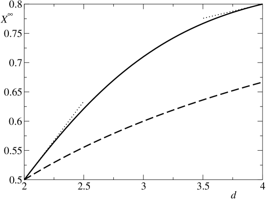
Figure 4: Asymptotic FDR $X^{\infty}_{\rm m}$ for the magnetization, for critical coarsening with nonzero initial magnetization. Solid line: Full theory (8.113) including non-Gaussian corrections; dotted lines indicate the first-order expansions near $d=2$ and 4. Dashed line: Gaussian theory (8.12).

In the opposite limit $d\to 2$, the $u$-integral in the definition (8.106) of $V_{d}$ diverges at the upper end; dropping all non-divergent corrections gives the leading divergence as

$$V_{d}\approx\int_{1}^{\infty}du\,\int_{0}^{1}dy\int_{0}^{1}dy^{\prime}\,(1-y-y^{\prime}+u)^{-d/2}\approx\int_{1}^{\infty}du\,u^{-d/2}=\frac{2}{d-2}$$ (8.117)

This divergence balances the vanishing prefactor $(d-2)/2$ in (8.108) and (8.113) whereas the contribution in the round brackets coming from $C_{\rm m}^{(1)}$ vanishes linearly with $d-2$. Consequently the asymptotic behaviour of the correlation function is, for $d$ close to $2$, $C_{\rm m}=[(d-2)/2]T_{\rm c}t_{\rm w}x^{-1}$ and the FDR becomes $X_{\rm m}^{\infty}=4/(d+6)=1/2$. One can also obtain the leading order correction in $\epsilon^{\prime}=d-2$, which is given by

$$X_{\rm m}^{\infty}=\frac{1}{2}+\left(\frac{1}{16}+\frac{\pi^{2}}{48}\right)\epsilon^{\prime}+{{\mathcal{O}}}(\epsilon^{\prime 2})$$ (8.118)

The only subtlety here is working out the subleading term of $V_{d}$. Setting $V_{d}=2/\epsilon^{\prime}+a_{0}+\ldots$, $a_{0}$ can be obtained as the limit for $d\to 2$ of (8.106) with $u^{-d/2}$ subtracted from the integrand. The limit can be taken in the integrand itself for finite $u$, giving a convergent integral with value $3/2-\pi^{2}/12$. But one has to account separately for the large-$u$ tail $u^{-d/2}[-1+\int dy\,dy^{\prime}(yy^{\prime})^{(d-2)/2}]$ which integrates to $(-1+4/d^{2})[2/(d-2)]\to-2$ for $d\to 2$, giving $a_{0}=-1/2-\pi^{2}/12$ overall.

In summary, the asymptotic magnetization FDR $X_{\rm m}^{\infty}$ decays from $4/5$ in $d=4$ to $1/2$ in $d=2$. Fig. 4 also shows numerical values for intermediate $d$. $X_{\rm m}^{\infty}$ is larger than the FDR (8.12) from the Gaussian theory except in the limit $d\to 2$; it also remains larger throughout than the FDR (3.3) for unmagnetized initial states, shown in Fig. 3.

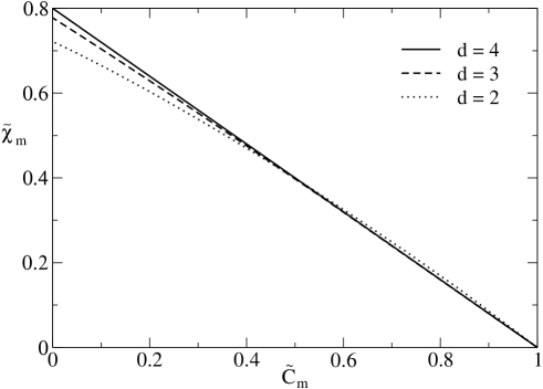
Figure 5: Normalized magnetization FD plot for $d=2,3,4$, showing normalized susceptibility $\tilde{\chi}_{\rm m}$ versus normalized correlation $\tilde{C}_{\rm m}$ in the limit of long times. For $d=4$ the plot is a straight line with (negative) slope $4/5$ as expected. Increasing deviations from this appear as $d$ decreases towards $2$.

We next turn to the shape of the FD plot for the magnetization. As explained in the introduction, this is obtained by plotting the normalized susceptibility $\tilde{\chi}_{\rm m}(t,t_{\rm w})=T_{\rm c}\chi_{\rm m}(t,t_{\rm w})/C_{\rm m}(t,t)$ versus $\tilde{C}_{\rm m}(t,t_{\rm w})=C_{\rm m}(t,t_{\rm w})/C_{\rm m}(t,t)$. In the limit $d\to 4$ the FD plot must be a straight line with slope $X_{\rm m}=4/5$, by continuity with the results for $d>4$. Numerical evaluation (see Fig. 5) shows that, as the dimensionality decreases, the FD plots deviate progressively from this straight lines. The most extreme case is the limit $d\to 2$, where analytical forms can be found.

To find the correlation function for $d\to 2$, it is useful to note that the scaling function ${\mathcal{F}}_{M}(x)$ becomes equal to $\delta(x-1)$ in the limit. Formally, one sees easily from (8.86) that for any smooth bounded function $f(x)$ and fixed $c>1$, $\int_{1}^{c}dx\,{\mathcal{F}}_{M}(x)f(x)\to f(1)$ because the divergence of ${\mathcal{F}}_{M}(x)$ at $x=1$ becomes non-integrable in $d=2$. We now exploit this to simplify $U$ from (8.104). In the first term in square brackets, the argument $xu/y_{\rm w}$ of ${\mathcal{F}}_{M}$ is always larger than $x/y_{\rm w}$ and hence than $1$ (except at the irrelevant boundary $y_{\rm w}=x$ of the $y_{\rm w}$-integral); in the limit $d\to 2$, this contribution therefore vanishes. In the second term, replacing ${\mathcal{F}}_{M}(x/uy_{\rm w})$ by $\delta(x/uy_{\rm w}-1)$ and expanding the prefactor to leading order in $(d-2)/2$ gives

$$\frac{U}{T_{\rm c}}=\frac{d-2}{2}\frac{x}{y_{\rm w}}\int_{0}^{1}dy\int_{0}^{1}dy^{\prime}\,(1-y-y^{\prime}+x/y_{\rm w})^{-1}$$ (8.119)

Performing the integrals over $y$ and $y^{\prime}$, one has

$$\frac{U}{T_{\rm c}}=\frac{d-2}{2}\frac{x}{y_{\rm w}}\left[\frac{x}{y_{\rm w}}\ln\left(1-\frac{y_{\rm w}^{2}}{x^{2}}\right)+\ln\left(\frac{x+y_{\rm w}}{x-y_{\rm w}}\right)\right]$$ (8.120)

We can now use this limit form of $U$ to get the contribution $C_{\rm m}^{(2)}$ to the correlation function; recall that $U$ was defined as the $u$-integral in (8.98). In the remaining $y_{\rm w}$-integral in this equation one can again replace ${\mathcal{F}}_{M}(1/y_{\rm w})$ by $\delta(1/y_{\rm w}-1)$ so that only $y_{\rm w}=1$ contributes, giving

$$C_{\rm m}=C_{\rm m}^{(2)}=\frac{d-2}{2}T_{\rm c}t_{\rm w}\left[x\ln\left(1-\frac{1}{x^{2}}\right)+\ln\left(\frac{x+1}{x-1}\right)\right]$$ (8.121)

One can show that the other contribution $C_{\rm m}^{(1)}$ to the magnetization correlator, given by (8.91), vanishes as $\sim(d-2)^{2}$ for $d\to 2$ so that to leading order $C_{\rm m}=C_{\rm m}^{(2)}$ as anticipated in writing (8.121). The corresponding response function is found by expanding (8.111) to leading order in $d-2$:

$$R_{\rm m}=\frac{d-2}{2}\ln\left(\frac{x}{x-1}\right)$$ (8.122)

To get the FDR it only remains to work out the $t_{\rm w}$-derivative of $C_{\rm m}$:

$$C_{\rm m}^{\prime}\ \ \equiv\ \ \partial_{t_{\rm w}}C_{\rm m} = \frac{d-2}{2}\,T_{\rm c}\ln\left(\frac{x+1}{x-1}\right)$$ (8.123)

We therefore get, for the full dependence of the limiting FDR for $d\to 2$ on scaled time $x=t/t_{\rm w}$

$$X_{\rm m}(x)=\frac{T_{\rm c}R_{\rm m}}{C_{\rm m}^{\prime}}=\ln\left(\frac{x}{x-1}\right)\left[\ln\!\left(\frac{x+1}{x-1}\right)\right]^{-1}$$ (8.124)

For $x\to\infty$ this gives $X_{\rm m}^{\infty}=1/2$ consistent with the discussion above. In the limit $x\to 1$ of comparable times, on the other hand, $X_{\rm m}(x)$ approaches 1, logarithmically slowly; the FD plot for $d\to 2$ therefore starts off with a pseudo-equilibrium slope. Interestingly, this implies that the trends of the slope with $d$ are different at the two ends of the plot: for well-separated times ($x\to\infty$), the slope decreases from $4/5$ to $1/2$ as $d$ decreases from 4 to 2; for comparable times ($x\to 1$) it increases from 4/5 to 1.

To get the FD plot itself we need the susceptibility, which is found by integration of the response (8.111) as

$$\chi_{\rm m}(t,t_{\rm w}) = \int_{t_{\rm w}}^{t}dt^{\prime}\,R_{\rm m}(t/t^{\prime})=t\int_{1/x}^{1}dz\,R_{\rm m}(1/z)$$ (8.125)

$$= t\int_{1/x}^{1}dz\,z^{(d-2)/4}\left[1-\left(1-z\right)^{(d-2)/2}\right]$$ (8.126)

Expanding to linear order in $d-2$ and integrating gives

$$\chi_{\rm m}(t,t_{\rm w})=\frac{d-2}{2}\,t\,\frac{x-1}{x}\left[1-\ln\left(\frac{x-1}{x}\right)\right]$$ (8.127)

The normalized susceptibility $\tilde{\chi}_{\rm m}$ is obtained by dividing by $C_{\rm m}(t,t)/T_{\rm c}$, which from (8.121) for $x\to 1$ equals $2\ln 2[(d-2)/2]\,t$. The resulting FD plot for $d\to 2$ is shown in Fig. 5, together with the ones for $d=3$ (determined numerically) and $d=4$. For $d\to 2$ the approach of the slope to the equilibrium value $X=1$ for $x\to 1$ is difficult to see because it is logarithmically slow. As expected from the trends with $d$ in the initial and final slopes of the FD plot, the curve for $d\to 2$ is the most strongly curved, while in $d=4$ we have the anticipated straight line with slope $4/5$ that is required by continuity with the results for $d>4$.

To quantify the shape of the FD plot further one can also consider the axis ratio $Y$, defined as the limiting value of $\tilde{\chi}_{\rm m}(t,t_{\rm w})=T_{\rm c}\chi_{\rm m}(t,t_{\rm w})/C_{\rm m}(t,t)$ for well-separated times $t\gg t_{\rm w}\gg 1$. In equilibrium this would correspond to the FDT for the static quantities, i.e. equal-time fluctuations and static susceptibilities. Out of equilibrium, if the FD plot is straight then $Y$ coincides with $X$; if it is not, then is has been argued that in some circumstances $Y$ can be more relevant for characterizing effective temperatures than $X$ [23]. For the magnetization FD plot in the current scenario of magnetized initial states, we see from Fig. 5 that $Y$ decreases along with $X_{\rm m}^{\infty}$ from $4/5$ as the dimension is lowered below $d=4$. The two quantities begin to differ more noticeably as $d$ decreases further, with $X_{\rm m}^{\infty}=1/2$ and $Y=1/(2\ln 2)=0.7213\ldots$ in the limit $d\to 2$.

9 Summary and discussion

In this paper we have considered the non-equilibrium dynamics of the spherical ferromagnet after a quench to the critical temperature $T_{\rm c}$. Our focus has been the calculation of correlation and response functions and the associated fluctuation-dissipation ratios (FDRs) $X(t,t_{\rm w})$. The key quantity that can be extracted from the latter is the asymptotic FDR $X^{\infty}$ for large and well-separated times $t\gg t_{\rm w}\gg 1$; it is independent of model-specific details within a given dynamical universality class. We were motivated by two questions: how does $X^{\infty}$ depend on the observable considered, both with regard to the lengthscale and the type of observable (spin, bond, spin product)? And what is the effect of initial conditions, in particular the presence of a nonzero magnetization in the initial state? The first question has implications for the interpretation of $T/X^{\infty}$ as an effective temperature, which is plausible only if this quantity is observable-independent. The second one allowed us to uncover whether different initial conditions can lead to different universality classes of critical coarsening.

A peculiarity of the spherical model is the weak infinite-range interaction produced by the spherical constraint. This requires that one distinguishes between long-range or “block” observables, which probe lengthscales large compared to the (time-dependent) correlation length but small compared to the system size, and global observables whose behaviour depends on correlations across the entire system. Technically, the first case is much easier to treat because the standard theory where the spins have Gaussian statistics can be used. Global correlation and response functions, on the other hand, require non-Gaussian corrections arising from the fluctuations of the effective Lagrange multiplier.

We dealt with the case of finite-range (i.e. either local or long-range) observables in Sec. 3. For spin observables, we found in the long-range case (3.3) the same $X^{\infty}$ as for local spin correlations and response [9]. This was as expected from the general correspondence between local and long-range observables discussed in the introduction. The FD plot for the long-range spin observable, i.e. the magnetization, is a straight line in the long-time limit. This is as in the Ising case in $d=1$ [10], but it is interesting to note that here it holds for all dimensions $d>2$. On the other hand, in the Ising model with $d\geq 2$, RG arguments have been adduced [11, 15, 17] to suggest that the magnetization FD plot should not be straight, though with deviations that are likely too small to be detectable numerically [15]. It is likely that the Gaussian statistics of the spherical model are responsible for producing a simpler, straight-line magnetization FD plot in all dimensions, although it would be interesting to know whether any other models have this property.

We then looked at the effect of the type of observable on $X^{\infty}$, considering both bond and spin product observables in either the local or long-range versions. The results in equations (3.15), (3.20), (3.26), (3.31) show that, although the precise time-dependence of $X(t,t_{\rm w})$ varies, the asymptotic FDR $X^{\infty}$ is the same in all cases. This is consistent with general arguments [13] suggesting that for a Gaussian theory all observables should yield the same $X^{\infty}$. In contrast to the Ising case [10], not all long-range observables give nontrivial FD plots; in fact, only the block product observable does so, and only for $d<4$, while all others produce pseudo-equilibrium FD plots for long times.

The bulk of the paper was concerned with the more challenging analysis of global correlation and response functions, focussing mostly on the energy as a key observable. In Sec. 4 we constructed a framework for calculating non-Gaussian corrections to the spins, which are ${{\mathcal{O}}}(N^{-1/2})$ to leading order. This lead to the general expression (4.11) for these leading-order corrections. It involves a two-time kernel $L(t,t_{\rm w})$ which from (4.9) is the functional inverse of $K(t,t_{\rm w})$ defined in (4.8). The basis of all subsequent calculations is the determination of the long-time scaling of these two functions, as summarized at the end of Sec. 4.2.

In Sec. 5 we obtained general expressions for energy correlation and response functions, in terms of the kernel $L$ and other quantities known from the Gaussian theory; the results can be found in eqs. (5.5,5.12,5.14,5.19) and (5.29). Evaluating these first for the equilibrium case, we found that the energy correlation and susceptibility display a plateau for $T$ just below $T_{\rm c}$ and $d>4$; this is caused by the $\mathbf{q}=\mathbf{0}$ wavevector, i.e. by the slow relaxation of the global magnetization. In Sec. 6, we proceeded to the long-time analysis of energy FD behaviour in the non-equilibrium case for $d>4$; the key results are (6.23) and (6.24). The associated FDR is given explicitly in (6.22) and has the same asymptotic value $X^{\infty}=1/2$ as for all other (finite-range) observables in $d>4$. The analysis of the case $d<4$ is more difficult, and we were able to find closed-form results (7.15,7.16) only in the limit of well-separated times $t/t_{\rm w}\gg 1$. This is, however, enough to determine $X^{\infty}$, with the result (7.19). Evaluating this, both numerically and by expansion in $4-d$ and $d-2$, the crucial conclusion is that it does not coincide with the asymptotic FDR for finite-range observables; see Fig. 3. A naive interpretation of $T/X^{\infty}$ as an effective temperature for critical coarsening dynamics is therefore ruled out, since such a temperaure ought to be observable-independent. On the other hand, to first order in $4-d$ the result agrees with an RG calculation [13] for the $O(n)$-model. We conclude that non-Gaussian corrections to the FD behaviour of global observables in the spherical model capture genuine physical effects that have close counterparts in more realistic systems with only short-range interactions.

Finally, in Sec. 8 we turned our attention to critical coarsening starting from magnetized initial states; physically this situation could be produced by an up-quench from an equilibrated state at a starting temperature $T<T_{\rm c}$. We concentrated on the simpler spin observables and found that already for them, the presence of a nonzero magnetization makes global properties sensitive to non-Gaussian corrections. As with the energy fluctuations, it is the global correlation and response functions that make contact with the results for short-range models, as obtained recently for the Ising case [20]: we find $X^{\infty}_{\rm m}=4/5$ for $d>4$, eq. (8.73). This is distinct from the value $X^{\infty}=1/2$ for the unmagnetized case, indicating that magnetized critical coarsening is in a separate dynamical universality class. Surprisingly, even the expressions for correlation and response functions themselves, which are not expected to be universal, coincide with those for the Ising case. It remains to be understood whether this is accidental or has more profound origins. For the case $d<4$, we obtained new exact values for the asymptotic FDR of magnetized critical coarsening. The magnetization response (8.111) can be found explicitly for long times, while for the magnetization correlator only the asymptotics for well-separated times (8.108) can be written in closed form. The resulting $X^{\infty}_{\rm m}$, eq. (8.113), is surprisingly nontrivial: while it matches continuously with $X^{\infty}_{\rm m}=4/5$ in $d>4$ and approaches the simple value $X^{\infty}_{\rm m}=1/2$ for $d\to 2$ as shown in Fig. 4, it is irrational already to first order in an expansion in $4-d$, eq. (8.116), or $d-2$, eq. (8.118).

While the conclusion of our calculation as regards the existence of a well-defined effective temperature for critical coarsening is negative, the issue of dynamic universality classes and new asymptotic FDRs due to magnetized (and possibly other, different) initial conditions clearly deserves further study. Results for systems with short-range interactions, such as the $O(n)$ and $n$-vector models, would be particularly welcome. After the present work was completed we became aware that a first step in this direction has recently been taken by the authors of Ref. [24], who calculated the FDR for the $n$-vector model with a magnetized initial state within an $\epsilon$-expansion around $d=2$. Intriguingly, their result $X^{\infty}=1/2$ for $d=2$ itself agrees with ours, but the first-order correction in $d-2$ remains rational even for $n\to\infty$. It therefore disagrees with our spherical model result (8.118). This appears to be the first example of genuine differences between the spherical and $n$-vector (with $n\to\infty$) models, which are known to have identical properties in equilibrium [25] and within a Gaussian theory of the dynamics.

As regards future work, we note first that a complete classification of dynamical universality classes within critical coarsening remains to be achieved. An earlier study of the spherical model considered initial conditions with long-range correlations but no overall magnetization; this yields no new (non-zero) values of the asymptotic FDR $X^{\infty}$ [26]. The presence of a non-zero magnetization thus appears to be important for observing new phenomena, and is reflected in our calculation by the fact that non-Gaussian fluctuations become important. Whether there are yet other initial conditions that could give rise to distinct values of $X^{\infty}$ is an open problem.

Our general framework for treating non-Gaussian corrections to the dynamics can also be applied in other contexts. For example, it can be used to analyse the fluctuations across thermal histories of correlation and response functions that have been coarse-grained across a finite-sized system. The properties of these fluctuations should be useful for understanding dynamical heterogeneities in coarsening dynamics [27], and we will report on the results of such a study shortly. We have also extended our approach to non-Gaussian corrections for the dynamics of e.g. the $O(n)$-model with large but finite $n$, opening up the attractive prospect of obtaining exact results analogous to the ones in this paper for models with exclusively short-range interactions.

Acknowledgements: We thank P Calabrese and A Gambassi for sharing their field theoretic results with us before publication, and for helpful discussions. PS acknowledges the hospitality of the KITP, Santa Barbara, where this research was supported in part by the NSF under grant no. PHY99-07949.

Appendix A Evaluation of $X_{E}^{\infty}$

In this appendix we evaluate the various numerical factors in the asymptotic FDR (7.18) for the energy in $d<4$. For $\beta_{d}$ we already have an expression (7.14). By definition, $\gamma_{d}$ is the large-$t$ limit of $CC(t,t)/t^{(4-d)/2}$. Its value can be deduced from (7.3): for small $q$, $q=\omega^{2}$ and hence $(dq)=\sigma_{d}d\omega\,\omega^{(d-2)/2}$. (The value of the proportionality constant, $\sigma_{d}=(4\pi)^{-d/2}\Gamma^{-1}(d/2)$, is not actually needed explicitly because it cancels from the overall result.) Thus from (7.3)

$$\gamma_{d}=\sigma_{d}T_{\rm c}^{2}\int\!dw\,w^{(d-6)/2}{\mathcal{F}}_{C}^{2}(w)$$ (1.1)

Next, $\lambda_{d}$ is defined by $L^{(2)}_{\rm eq}(t)=\lambda_{d}t^{(d-6)/2}$ for large $t$. The Laplace transform ot $L^{(2)}_{\rm eq}$ therefore has a singular term $\hat{L}^{(2)}_{\rm eq}(s)=\lambda_{d}\Gamma((d-4)/2)s^{(4-d)/2}$ for $s\to 0$. From (4.21), this must match the corresponding singularity in $-1/\hat{K}_{\rm eq}(s)$. The latter follows from (4.22) as $\hat{K}_{\rm eq}(s)=s^{(d-4)/2}T_{\rm c}\sigma_{d}\int\!dw\,w^{(d-4)/2}(1+2w)^{-1}=s^{(d-4)/2}T_{\rm c}\sigma_{d}2^{(2-d)/2}\Gamma((4-d)/2)\Gamma((d-2)/2)$. This tells us that

$$\lambda_{d}^{-1}=-T_{\rm c}\sigma_{d}2^{(2-d)/2}\Gamma\left({\textstyle\frac{4-d}{2}}\right)\Gamma\left({\textstyle\frac{d-4}{2}}\right)\Gamma\left({\textstyle\frac{d-2}{2}}\right)$$ (1.2)

Finally, we need $\alpha_{d}$ from (7.13). Inserting (2.25) into (7.7) and using (1.1), the scaling function ${\mathcal{G}}(x)$ can be written for $x\geq 1$ as

$${\mathcal{G}}(x) = \frac{4\sigma_{d}T_{\rm c}^{2}}{\gamma_{d}}\int dw\,w^{(d-6)/2}w^{2}\int_{0}^{1}dy\int_{0}^{1}dy^{\prime}(yy^{\prime})^{(d-4)/2}e^{-2(1+x-y-y^{\prime})w}$$ (1.3)

$$= \frac{\Gamma(\frac{d}{2})2^{(4-d)/2}\sigma_{d}T_{\rm c}^{2}}{\gamma_{d}}\int_{0}^{1}dy\,y^{(d-4)/2}\int_{0}^{1}\frac{dy^{\prime}}{y^{\prime 2}}[(1+x-y)/y^{\prime}-1]^{-d/2}$$ (1.4)

$$= \frac{2}{d-2}\frac{\Gamma(\frac{d}{2})2^{(4-d)/2}\sigma_{d}T_{\rm c}^{2}}{\gamma_{d}}\int_{0}^{1}dy\,y^{(d-4)/2}\frac{(x-y)^{(2-d)/2}}{1+x-y}$$ (1.5)

We define the integral as $\tilde{\mathcal{G}}(x)$. It is an unnormalized version of ${\mathcal{G}}(x)$; because of ${\mathcal{G}}(1)=1$ one then has ${\mathcal{G}}(x)=\tilde{\mathcal{G}}(x)/\tilde{\mathcal{G}}(1)$. The corresponding unnormalized value of $\alpha_{d}$, $\tilde{\alpha}_{d}=\alpha_{d}\tilde{\mathcal{G}}(1)$, is

$$\tilde{\alpha}_{d} = \int_{0}^{\infty}dx\,x\left[\tilde{g}_{d}x^{-d/2}-\tilde{\mathcal{G}}(x)\right]$$ (1.6)

$$= \frac{2\tilde{g}_{d}}{4-d}-\int_{0}^{1}dx\,x\tilde{\mathcal{G}}(x)+\int_{1}^{\infty}dx\,x\left[\tilde{g}_{d}x^{-d/2}-\tilde{\mathcal{G}}(x)\right]$$ (1.7)

$$= \frac{4}{(4-d)(d-2)}-\int_{1}^{\infty}dx\,x^{-(d+2)/2}\tilde{\mathcal{G}}(x)+\int_{1}^{\infty}dx\,x\left[\frac{2x^{-d/2}}{d-2}-\tilde{\mathcal{G}}(x)\right]$$ (1.8)

Here we have used (7.7) to express the values of $\tilde{\mathcal{G}}(x)$ for $x<1$ in terms of those for $x>1$; we also inserted $\tilde{g}_{d}=g_{d}\tilde{\mathcal{G}}(1)=\lim_{x\to\infty}\tilde{\mathcal{G}}(x)x^{d/2}=2/(d-2)$ which follows from (1.5). The first integral has no divergences. The second one could in principle be left as it is for numerical evaluation, but it is useful to rewrite it using a dimensional regularization trick, as follows. If we extend the definition of $\tilde{\mathcal{G}}(x)$ to $d>4$ using (1.5), then both parts of the second integral in (1.8) are separately finite for $4<d<6$, and we can evaluate them first in that range of $d$ and then analytically continue to $d<4$. (The region $x\approx 1$ causes no difficulty since $\tilde{\mathcal{G}}(x)\sim(x-1)^{(4-d)/2}$ for $x\to 1$, which remains integrable for $d<6$.) The first part gives $[2/(d-2)][2/(d-4)]$ and just cancels the first term in (1.8), so that

$$\int_{1}^{\infty}dx\,x\left[\frac{2x^{-d/2}}{d-2}-\tilde{\mathcal{G}}(x)\right]+\frac{4}{(4-d)(d-2)}=$$ (1.9)

$$= -\int_{1}^{\infty}dx\int_{0}^{1}dy\,y^{(d-4)/2}(x-y)^{(2-d)/2}\frac{x}{1+x-y}$$

$$= -\frac{\pi}{\sin[\pi(d-4)/2]}+\int_{1}^{\infty}dx\int_{0}^{1}dy\,y^{(d-4)/2}\frac{(x-y)^{(2-d)/2}(1-y)}{1+x-y}$$ (1.10)

The cancellation of the pure power-law term proportional to $\tilde{g}_{d}$ from the integral (7.13) is a feature well-known from dimensional regularization in field theory. Inserting the last expression into (1.8) then gives (7.20) in the main text.

Collecting the above results, the asymptotic FDR (7.18) for the energy in $d<4$ is

$$X_{E}^{\infty} = \frac{4T_{\rm c}}{d\tilde{\alpha}_{d}}\Biggl{[}\frac{2}{d-2}\frac{\Gamma\left(\frac{d}{2}\right)2^{(4-d)/2}\sigma_{d}T_{\rm c}^{2}}{\gamma_{d}}\left(-\frac{\Gamma\left(\frac{d-4}{2}\right)\Gamma\left(\frac{d+4}{2}\right)}{\Gamma(d)}\right)\gamma_{d}\Biggr{]}^{-1}$$ (1.11)

$$\times\left[-T_{\rm c}\sigma_{d}2^{(2-d)/2}\Gamma{\textstyle\left(\frac{4-d}{2}\right)}\Gamma{\textstyle\left(\frac{d-4}{2}\right)}\Gamma{\textstyle\left(\frac{d-2}{2}\right)}\right]$$

$$= \frac{2}{d\tilde{\alpha}_{d}}\frac{\Gamma(d)\Gamma{\textstyle\left(\frac{4-d}{2}\right)}}{\Gamma\left(\frac{d+4}{2}\right)}$$ (1.12)

which is the result stated in (7.19).

Appendix B Solution for ${\mathcal{F}}_{L}(x)$ for magnetized case in $d<4$

In this appendix we prove that the solution ${\mathcal{F}}_{L}(x)=2/(4-d)x^{(2-d)/2}+(2-d)/(4-d)x^{-d/2}$ given in (8.81) does indeed satisfy the integral equation (4.34)

$$\int_{1}^{x}dy\,(x-y)^{(2-d)/2}(y-1)^{(d-6)/2}\left[{\mathcal{F}}_{K}\left({x}/{y}\right){\mathcal{F}}_{L}\left(y\right)-{\mathcal{F}}_{K}(x)\right]=0$$ (2.1)

with $d<4$ and ${\mathcal{F}}_{K}(x)$ given by (8.78) for the magnetized case considered here.

The difference in the square brackets can be written as the integral of a partial derivative

$${\mathcal{F}}_{K}\left({x}/{y}\right){\mathcal{F}}_{L}\left(y\right)-{\mathcal{F}}_{K}(x)=\int_{1}^{y}dz\,\partial_{z}\left[{\mathcal{F}}_{K}\left({x}/{z}\right){\mathcal{F}}_{L}\left(z\right)\right]$$ (2.2)

so that, after exchanging the order of the integrals, the left-hand side of (2.1) becomes

$$l = \int_{1}^{x}dz\,\partial_{z}\left[{\mathcal{F}}_{K}(x/z){\mathcal{F}}_{L}(z)\right]\int_{z}^{x}dy\,(x-y)^{(2-d)/2}(y-1)^{(d-6)/2}$$ (2.3)

$$= \frac{1}{x-1}\frac{2}{4-d}\int_{1}^{x}dz\,(x-z)^{(4-d)/2}(z-1)^{(d-4)/2}\partial_{z}\left[{\mathcal{F}}_{K}(x/z){\mathcal{F}}_{L}\left(z\right)\right]$$ (2.4)

where in the second step the $y$-integral has been performed. Eq. (2.4) can equivalently be obtained from (2.1) by integrating by parts. From (8.78) for ${\mathcal{F}}_{K}(x)$ and the form given above for ${\mathcal{F}}_{L}(x)$, we can find the $z$-derivative of ${\mathcal{F}}_{K}\left({x}/{z}\right){\mathcal{F}}_{L}(z)$ explicitly. After simplifying the latter, equation (2.4) becomes

$$l = \eta\int_{1}^{x}dz\,(x-z)^{(4-d)/2}(z-1)^{(d-4)/2}\left\{-\frac{1}{z}+\frac{d}{2z^{2}}\right.+\frac{d-2}{2}\left[\frac{d}{2}x-z(x+1)\right]$$ (2.5)

$$\times\left.z^{-(d+2)/2}(x-z)^{(d-4)/2}\int_{z/x}^{1}dy\,(1-y)^{(2-d)/2}y^{(d-4)/2}\right\}$$

where

$$\eta=\frac{x^{(2-d)/2}}{x-1}\frac{2(d-2)}{(4-d)^{2}}$$ (2.6)

collects all the prefactors. By rescaling $y$ by a factor $x$, the last integral in (2.5) can be transformed to $\int_{z}^{x}dy\,(x-y)^{(2-d)/2}y^{(d-4)/2}$. Interchanging the $y$ and $z$-integrals then gives

$$\frac{l}{\eta} = \int_{1}^{x}dz\,(x-z)^{(4-d)/2}(z-1)^{(d-4)/2}\left(-\frac{1}{z}+\frac{d}{2z^{2}}\right)$$ (2.7)

$$+\int_{1}^{x}dy\,(x-y)^{(2-d)/2}y^{(d-4)/2}$$

$$\times\int_{1}^{y}dz\,z^{-(d+2)/2}(z-1)^{(d-4)/2}\,\frac{d-2}{2}\left[\frac{d}{2}x-z(x+1)\right]$$

The integral on the last line can now be calculated explicitly to give

$$g(y) = \left(\frac{y-1}{y}\right)^{(d-2)/2}\left(\frac{d-2}{2}\frac{x}{y}-1\right)$$ (2.8)

Relabelling $y$ to $z$, eq. (2.7) can thus be written as a single integral:

$$\frac{l}{\eta} = \int_{1}^{x}dz\,(x-z)^{(2-d)/2}\left[(z-1)^{(d-4)/2}(x-z)\left(-\frac{1}{z}+\frac{d}{2z^{2}}\right)+z^{(d-4)/2}g(z)\right]$$ (2.9)

$$= \int_{1}^{x}dz\,(x-z)^{(2-d)/2}(z-1)^{(d-4)/2}\left[\frac{x}{z^{2}}-\left(\frac{d-2}{2}+\frac{4-d}{2}x\right)\frac{1}{z}\right]$$ (2.10)

Finally, the variable change $v=(x/z-1)/(x-1)$ transforms the integration range to $0\ldots 1$ and leads after a few simplifications to straightforward Beta-function integrals:

$$\frac{l}{\eta} = x^{(2-d)/2}(x-1)\int_{0}^{1}dv\,v^{(2-d)/2}\left(-\frac{4-d}{2}+v\right)(1-v)^{(d-4)/2}$$ (2.11)

$$= x^{(2-d)/2}(x-1)\left[-\frac{4-d}{2}\frac{\Gamma\left(\textstyle\frac{4-d}{2}\right)\Gamma\left(\textstyle\frac{d-2}{2}\right)}{\Gamma(1)}+\frac{\Gamma\left(\textstyle\frac{6-d}{2}\right)\Gamma\left(\textstyle\frac{d-2}{2}\right)}{\Gamma(2)}\right]=0$$ (2.12)

This proves that (2.1) is indeed satisfied, as required.

References

References

- [1] L F Cugliandolo, J Kurchan, and L Peliti. Energy flow, partial equilibration, and effective temperatures in systems with slow dynamics. Phys. Rev. E, 55(4):3898–3914, 1997.
- [2] A Crisanti and F Ritort. Violation of the fluctuation-dissipation theorem in glassy systems: basic notions and the numerical evidence. J. Phys. A, 36(21):R181–R290, 2003.
- [3] J P Bouchaud, L F Cugliandolo, J Kurchan, and M Mézard. Out of equilibrium dynamics in spin-glasses and other glassy systems. In A P Young, editor, Spin glasses and random fields, pages 161–223, Singapore, 1998. World Scientific.
- [4] L E Reichl. A modern course in statistical physics. University of Texas Press, Austin, 1980.
- [5] L F Cugliandolo and J Kurchan. Analytical solution of the off-equilibrium dynamics of a long- range spin-glass model. Phys. Rev. Lett., 71(1):173–176, 1993.
- [6] L F Cugliandolo and J Kurchan. On the out-of-equilibrium relaxation of the Sherrington- Kirkpatrick model. J. Phys. A, 27(17):5749–5772, 1994.
- [7] S Fielding and P Sollich. Observable dependence of fluctuation-dissipation relations and effective temperatures. Phys. Rev. Lett., 88:050603, 2002.
- [8] P Sollich, S Fielding, and P Mayer. Fluctuation-dissipation relations and effective temperatures in simple non-mean field systems. J. Phys. Cond. Matt., 14(7):1683–1696, 2002.
- [9] C Godrèche and J M Luck. Response of non-equilibrium systems at criticality: ferromagnetic models in dimension two and above. J. Phys. A, 33(50):9141–9164, 2000.
- [10] P Mayer, L Berthier, J P Garrahan, and P Sollich. Fluctuation-dissipation relations in the nonequilibrium critical dynamics of Ising models. Phys. Rev. E, 68:016116, 2003.
- [11] P Calabrese and A Gambassi. Ageing properties of critical systems. J. Phys. A, 38(18):R133–R193, 2005.
- [12] A J Bray. Theory of phase-ordering kinetics. Adv. Phys., 43(3):357–459, 1994.
- [13] P Calabrese and A Gambassi. On the definition of a unique effective temperature for non- equilibrium critical systems. JSTAT, page P07013, 2004.
- [14] P Mayer and P Sollich. General solutions for multispin two-time correlation and response functions in the Glauber-Ising chain. J. Phys. A, 37(1):9–49, 2004.
- [15] P Mayer, L Berthier, J P Garrahan, and P Sollich. Reply to comment on ‘fluctuation-dissipation relations in the nonequilibrium critical dynamics of Ising models’. Phys. Rev. E, 70:018102, 2004.
- [16] P Calabrese and A Gambassi. Aging in ferromagnetic systems at criticality near four dimensions. Phys. Rev. E, 65:066120, 2002.
- [17] P Calabrese and A Gambassi. Two-loop critical fluctuation-dissipation ratio for the relaxational dynamics of the O(n) Landau-Ginzburg Hamiltonian. Phys. Rev. E, 66:066101, 2002.
- [18] T H Berlin and M Kac. Phys. Rev. E, 86:821, 1952.
- [19] G S Joyce. Critical properties of the spherical model. In C Domb and M S Green, editors, Phase Transitions and Critical Phenomena, Vol. 2, chapter 10, pages 375–442. Academic, London, 1972.
- [20] A Garriga, P Sollich, I Pagonabarraga, and F Ritort. Universality of fluctuation-dissipation ratios: The ferromagnetic model. Phys. Rev. E, 2005. To appear; available as cond-mat/0508243.
- [21] F Corberi, E Lippiello, and M Zannetti. Scaling of the linear response function from zero-field-cooled and thermoremanent magnetization in phase-ordering kinetics. Phys. Rev. E, 68:046131, 2003.
- [22] A Annibale. PhD thesis, King’s College London.
- [23] C S O’Hern, A J Liu, and S R Nagel. Effective temperatures in driven systems: static versus time- dependent relations. Phys. Rev. Lett., 93:165702, 2004.
- [24] A A Fedorenko and S Trimper. Critical aging of heisenberg ferromagnet from a completely ordered state. Preprint cond-mat/0507112.
- [25] H E Stanley. Spherical model as the limit of infinite spin dimensionality. Phys. Rev., 176(1):718–722, 1968.
- [26] A Picone and M Henkel. Response of non-equilibrium systems with long-range initial correlations. J. Phys. A, 35(27):5575–5590, 2002.
- [27] H E Castillo, C Chamon, L F Cugliandolo, J L Iguain, and M P Kennett. Spatially heterogeneous ages in glassy systems. Phys. Rev. B, 68:134442, 2003.