Resonant proximity effect in normal metal / diffusive ferromagnet / superconductor junctions

Abstract

Resonant proximity effect in the normal metal / insulator / diffusive ferromagnet / insulator / $s$- and $d$-wave superconductor (N/I/DF/I/S) junctions is studied for various regimes by solving the Usadel equation with the generalized boundary conditions. Conductance of the junction and the density of states in the DF layer are calculated as a function of the insulating barrier heights at the interfaces, the magnitudes of the resistance, Thouless energy and the exchange field in DF and the misorientation angle $\alpha$ of a $d$-wave superconductor. It is shown that the resonant proximity effect originating from the exchange field in DF layer strongly modifies the tunneling conductance and density of states. We have found that, due to the resonant proximity effect, for $s$-wave junctions a sharp zero bias conductance peak (ZBCP) appears for small Thouless energy, while a broad ZBCP appears for large Thouless energy. The magnitude of this ZBCP can exceed the normal state conductance in contrast to the case of diffusive normal metal / superconductor junctions. Similar structures exist in the density of states in the DF-layer. For $d$-wave junctions at $\alpha=0$, similar structures are predicted in the conductance and the density of states. With the increase of the angle $\alpha$, the magnitude of the resonant ZBCP decreases due to the formation of the mid gap Andreev resonant states.

I Introduction

There is a continuously growing interest in the physics of charge and spin transport in ferromagnet / superconductor (F/S) junctions. One of the applications of F/S junctions is determination of the spin polarization of the F layer. Analyzing signatures of Andreev reflection Andreev in differential conductance by a modified Blonder, Tinkham and Klapwijk (BTK) theoryBTK , one can estimate the spin polarization of the F layer Tedrow ; Upadhyay ; Soulen ; Mazin ; Nadgorny ; Belzig1 . This method was generalized and applied to ferromagnet / unconventional superconductor junctionsFS . Most of these works are applicable to ballistic ferromagnets while understanding of physics in contacts between diffusive ferromagnets (DF) and (both conventional and unconventional) superconductors (S) is not complete yet. The model should also properly take into account the proximity effect in the DF/S system.

In DF/S junctions Cooper pairs penetrating into the DF layer from the S layer have nonzero momentum due to the exchange fieldBuzdin1982 ; Buzdin1991 ; Demler ; buzdinrev ; golubov ; bverev . This property results in many interesting phenomenaRyazanov ; Kontos1 ; Blum ; Sellier ; Strunk ; Radovic ; Tagirov ; Fominov ; Rusanov ; Ryazanov1 ; Kadigrobov ; Leadbeater ; Seviour2 ; Bergeret ; Kadigrobov2 . One interesting consequence of the oscillations of the pair amplitude is spatially damped oscillating behavior of the density of states (DOS) in a ferromagnet predicted theoretically Buzdin ; Baladie ; Zareyan ; Bergeret2 . In a strong ferromagnet the exchange field breaks the induced Cooper pairs, while for a weak exchange field the pair amplitude can be enhanced and the energy dependent DOS can have a zero-energy peak Zareyan ; Baladie ; Bergeret2 ; Krivoruchko ; Golubov3 ; Kontos . Since DOS is a fundamental quantity, this resonant proximity effect can influence various transport phenomena. In our recent paper Yoko2 the DOS peak was studied in two regimes of weak and strong proximity effect and the conditions for the appearance of this DOS anomaly were clarified. However, its consequence for the junction conductance was not systematically investigated so far.

It is known that in contacts involving unconventional superconductors the so-called zero-bias conductance peak (ZBCP) takes place due to the formation of the midgap Andreev resonant states (MARS) Buch ; TK95 ; Kashi00 ; Experiments . An interplay of the resonant proximity effect with MARS in DF/$d$-wave superconductor (DF/D) junctions is an interesting subject which deserves theoretical study.

The purpose of the present paper is to formulate theoretical model for the proximity effect in the normal metal/DF/$s$- and $d$-wave superconductor (N/I/DF/I/S) junctions and to study the influence of the resonant proximity effect due to the exchange field on the tunneling conductance and the DOS. A number of physical phenomena may coexist in these structures such as impurity scattering, oscillating pair amplitude, phase coherence and MARS. We will employ the quasiclassical Usadel equations Usadel with the Kupriyanov-Lukichev boundary conditions KL generalized by Nazarov within the circuit theory Nazarov2 . The generalized boundary conditions are relevant for the actual junctions when the barrier transparency is not small. New physical phenomena regarding zero-bias conductance are properly described within this approach, e.g., the crossover from a ZBCP to a zero bias conductance dip (ZBCD). The generalized boundary conditions were recently applied to the study of contacts of diffusive normal metals (DN) with conventional TGK and unconventional superconductors Nazarov3 ; Golubov2 ; p-wave . Here we consider the case of N/I/DF/I/S junctions with a weak ferromagnet having small exchange field comparable with the superconducting gap. SF contacts with weak ferromagnets were realized in recent experiments with, e.g., CuNi alloys Ryazanov , Ni doped PdKontos or magnetic semiconductors. Therefore, our results are applicable to these materials and may be observed experimentally.

The normalized conductance of the N/I/DF/I/S) junction $\sigma_{T}(eV)=\sigma_{S}(eV)/\sigma_{N}(eV)$ will be studied as a function of the bias voltage $V$, where $\sigma_{S(N)}(eV)$ is the tunneling conductance in the superconducting (normal) state. We will consider the influence of various parameters on $\sigma_{T}(eV)$, such as the height of the interface insulating barriers, the resistance $R_{d}$, the exchange field $h$ and the Thouless energy $E_{Th}$ in the DF layer. In the case of $\ d$-wave superconductor, important parameter is the angle between the normal to the interface and the crystal axis of $d$-wave superconductor $\alpha$. Throughout the paper we confine ourselves to zero temperature and put $k_{B}=\hbar=1$.

The organization of this paper is as follows. In section II, we will provide the detailed derivation of the expression for the normalized tunneling conductance. In section III, the results of calculations are presented for various types of junctions. In section IV, the summary of the obtained results is given.

II Formulation

In this section we introduce the model and the formalism. We consider a junction consisting of normal and superconducting reservoirs connected by a quasi-one-dimensional diffusive ferromagnet conductor (DF) with a length $L$ much larger than the mean free path. The interface between the DF conductor and the S electrode has a resistance $R_{b}$ while the DF/N interface has a resistance $R_{b}^{\prime}$. The positions of the DF/N interface and the DF/S interface are denoted as $x=0$ and $x=L$, respectively. We model infinitely narrow insulating barriers by the delta function $U(x)=H\delta(x-L)+H^{\prime}\delta(x)$. The resulting transparency of the junctions $T_{m}$ and $T_{m}^{\prime}$ are given by $T_{m}=4\cos^{2}\phi/(4\cos^{2}\phi+Z^{2})$ and $T_{m}^{\prime}=4\cos^{2}\phi/(4\cos^{2}\phi+{Z^{\prime}}^{2})$, where $Z=2H/v_{F}$ and $Z^{\prime}=2H^{\prime}/v_{F}$ are dimensionless constants and $\phi$ is the injection angle measured from the interface normal to the junction and $v_{F}$ is Fermi velocity.

We apply the quasiclassical Keldysh formalism in the following calculation of the tunneling conductance. The 4 $\times$ 4 Green’s functions in N, DF and S are denoted by $\check{G}_{0}(x)$, $\check{G}_{1}(x)$ and $\check{G}_{2}(x)$ respectively where the Keldysh component $\hat{K}_{0,1,2}(x)$ is given by $\hat{K}_{i}(x)=\hat{R}_{i}(x)\hat{f}_{i}(x)-\hat{f}_{i}(x)\hat{A}_{i}(x)$ with retarded component $\hat{R}_{i}(x)$, advanced component $\hat{A}_{i}(x)=-\hat{R}_{i}^{\ast}(x)$ using distribution function $\hat{f}_{i}(x)(i=0,1,2)$. In the above, $\hat{R}_{0}(x)$ is expressed by $\hat{R}_{0}(x)=\hat{\tau}_{3}$ and $\hat{f}_{0}(x)=f_{l0}+\hat{\tau}_{3}f_{t0}$. $\hat{R}_{2}(x)$ is expressed by $\hat{R}_{2}(x)=g\hat{\tau}_{3}+f\hat{\tau}_{2}$ with $g=\epsilon/\sqrt{\epsilon^{2}-\Delta^{2}}$ and $f=\Delta/\sqrt{\Delta^{2}-\epsilon^{2}}$, where $\hat{\tau}_{2}$ and $\hat{\tau}_{3}$ are the Pauli matrices, and $\varepsilon$ denotes the quasiparticle energy measured from the Fermi energy and $\hat{f}_{2}(x)=\tanh(\epsilon/2T)$ in thermal equilibrium with temperature $T$. We put the electrical potential zero in the S-electrode. In this case the spatial dependence of $\check{G}_{1}(x)$ in DF is determined by the static Usadel equation Usadel ,

$$D\frac{\partial}{\partial x}[\check{G}_{1}(x)\frac{\partial\check{G}_{1}(x)}{\partial x}]+i[\check{H},\check{G}_{1}(x)]=0$$ (1)

with the diffusion constant $D$ in DF. Here $\check{H}$ is given by

$$\check{H}=\left(\begin{array}[]{cc}\hat{H}_{0}&0\\ 0&\hat{H}_{0}\end{array}\right),$$

with $\hat{H}_{0}=(\epsilon-(+)h)\hat{\tau}_{3}$ for majority(minority) spin where $h$ denotes the exchange field. Note that we assume a weak ferromagnet and neglect the difference of Fermi velocity between majority spin and minority spin. The Nazarov’s generalized boundary condition for $\check{G}_{1}(x)$ at the DF/S interface is given in Refs.TGK ; Golubov2 . The generalized boundary condition for $\check{G}_{1}(x)$ at the DF/N interface has the form:

$$\frac{L}{R_{d}}(\check{G}_{1}\frac{\partial\check{G}_{1}}{\partial x})_{\mid x=0_{+}}=-{R_{b}^{\prime}}^{-1}<B>^{\prime},$$ (2)

$$B=\frac{2T_{m}^{\prime}[\check{G}_{0}(0_{-}),\check{G}_{1}(0_{+})]}{4+T_{m}^{\prime}([\check{G}_{0}(0_{-}),\check{G}_{1}(0_{+})]_{+}-2)}.$$

The average over the various angles of injected particles at the interface is defined as

$$<B(\phi)>^{(\prime)}=\frac{\int_{-\pi/2}^{\pi/2}d\phi\cos\phi B(\phi)}{\int_{-\pi/2}^{\pi/2}d\phi T^{(\prime)}(\phi)\cos\phi}$$

with $B(\phi)=B$ and $T^{(\prime)}(\phi)=T_{m}^{(\prime)}$. The resistance of the interface $R_{b}$ is given by

$$R_{b}^{(\prime)}=R_{0}^{(\prime)}\frac{2}{\int_{-\pi/2}^{\pi/2}d\phi T^{(\prime)}(\phi)\cos\phi}.$$

Here $R_{0}^{(\prime)}$ is Sharvin resistance given by $R_{0}^{(\prime)-1}=e^{2}k_{F}^{2}S_{c}^{(\prime)}/(4\pi^{2})$ in the three-dimensional case.

The electric current per spin direction is expressed using $\check{G}_{1}(x)$ as

$$I_{el}=\frac{-L}{8eR_{d}}\int_{0}^{\infty}d\epsilon\mathrm{Tr}[\hat{\tau_{3}}(\check{G}_{1}(x)\frac{\partial\check{G}_{1}(x)}{\partial x})^{K}],$$ (3)

where $(\check{G_{1}}(x)\frac{\partial\check{G_{1}}(x)}{\partial x})^{K}$ denotes the Keldysh component of $(\check{G_{1}}(x)\frac{\partial\check{G_{1}}(x)}{\partial x})$. In the actual calculation it is convenient to use the standard $\theta$-parameterization where function $\hat{R}_{1}(x)$ is expressed as $\hat{R}_{1}(x)=\hat{\tau}_{3}\cos\theta(x)+\hat{\tau}_{2}\sin\theta(x).$ The parameter $\theta(x)$ is a measure of the proximity effect in DF.

The distribution function $\hat{f}_{1}(x)$ is given by $\hat{f}_{1}(x)=f_{l}(x)+\hat{\tau}_{3}f_{t}(x)$ where the component $f_{t}(x)$ determines the conductance of the junction we are now concentrating on. From the retarded or advanced component of the Usadel equation, the spatial dependence of $\theta(x)$ is determined by the following equation

$$D\frac{\partial^{2}}{\partial x^{2}}\theta(x)+2i(\epsilon-(+)h)\sin[\theta(x)]=0$$ (4)

for majority(minority) spin, while for the Keldysh component we obtain

$$D\frac{\partial}{\partial x}[\frac{\partial f_{t}(x)}{\partial x}\mathrm{cosh^{2}}\theta_{im}(x)]=0.$$ (5)

At $x=0$, since $f_{t0}$ is the distribution function in the normal electrode given by

$$f_{t0}=\frac{1}{2}\{\tanh[(\epsilon+eV)/(2T)]-\tanh[(\epsilon-eV)/(2T)]\}.$$

Next we focus on the boundary condition at the DF/N interface. Taking the retarded part of Eq. (2), we obtain

$$\frac{L}{R_{d}}\frac{\partial\theta(x)}{\partial x}\mid_{x=0_{+}}=\frac{<F>^{\prime}}{R_{b}^{\prime}}$$ (6)

$$F=\frac{2T_{m}^{\prime}\sin\theta_{0}}{(2-T_{m}^{\prime})+T_{m}^{\prime}\cos\theta_{0}},$$

with $\theta_{0}=\theta(0_{+})$.

On the other hand, from the Keldysh part of Eq. (2), we obtain

$$\frac{L}{R_{d}}(\frac{\partial f_{t}}{\partial x})\mathrm{{\cosh^{2}}}\theta_{im}(x)\mid_{x=0_{+}}=-\frac{<I_{b1}>^{\prime}(f_{t0}-f_{t}(0_{+}))}{R_{b}^{\prime}},$$ (7)

with

$$I_{b1}=\frac{T_{m}^{\prime 2}\Lambda_{1}^{\prime}+2T_{m}^{\prime}(2-T_{m}^{\prime})\mathrm{{Real}\{\cos\theta_{0}\}}}{\mid(2-T_{m}^{\prime})+T_{m}^{\prime}\cos\theta_{0}\mid^{2}}$$

$$\Lambda_{1}^{\prime}=(1+\mid\cos\theta_{0}\mid^{2}+\mid\sin\theta_{0}\mid^{2}).$$

Finally, we obtain the following final result for the electric current through the contact

$$I_{el}=\frac{1}{2e}\int_{0}^{\infty}d\epsilon\frac{f_{t0}}{\frac{R_{b}}{<I_{b0}>}+\frac{R_{d}}{L}\int_{0}^{L}\frac{dx}{\cosh^{2}\theta_{im}(x)}+\frac{R_{b}^{\prime}}{<I_{b1}>^{\prime}}}.$$ (8)

Then the differential resistance $R$ per one spin projection at zero temperature is given by

$$R=\frac{2R_{b}}{<I_{b0}>}+\frac{2R_{d}}{L}\int_{0}^{L}\frac{dx}{\cosh^{2}\theta_{im}(x)}+\frac{2R_{b}^{\prime}}{<I_{b1}>^{\prime}}$$ (9)

with

$$I_{b0}=\frac{T_{m}^{2}\Lambda_{1}+2T_{m}(2-T_{m})\Lambda_{2}}{2\mid(2-T_{m})+T_{m}[g\cos\theta_{L}+f\sin\theta_{L}]\mid^{2}},$$

$$\Lambda_{1}=(1+\mid\cos\theta_{L}\mid^{2}+\mid\sin\theta_{L}\mid^{2})(\mid g\mid^{2}+\mid f\mid^{2}+1)$$

$$+4\mathrm{Imag}[fg^{*}]\mathrm{Imag}[\cos\theta_{L}\sin\theta_{L}^{*}],$$ (10)

$$\Lambda_{2}=\mathrm{{Real}\{g(\cos\theta_{L}+\cos\theta_{L}^{*})+f(\sin\theta_{L}+\sin\theta_{L}^{*})\}}.$$ (11)

This is an extended version of the Volkov-Zaitsev-Klapwijk formula Volkov . For a $d$-wave junction, the function $I_{b0}$ is given by the following expressionGolubov2

$$I_{b0}=\frac{T_{m}}{2}\frac{C_{0}}{\mid(2-T_{m})(1+g_{+}g_{-}+f_{+}f_{-})+T_{m}[\cos\theta_{L}(g_{+}+g_{-})+\sin\theta_{L}(f_{+}+f_{-})]\mid^{2}}$$

$$C_{0}=T_{m}(1+\mid\cos\theta_{L}\mid^{2}+\mid\sin\theta_{L}\mid^{2})[\mid g_{+}+g_{-}\mid^{2}+\mid f_{+}+f_{-}\mid^{2}+\mid 1+f_{+}f_{-}+g_{+}g_{-}\mid^{2}+\mid f_{+}g_{-}-g_{+}f_{-}\mid^{2}]$$

$$+2(2-T_{m})\mathrm{Real}\{(1+g_{+}^{*}g_{-}^{*}+f_{+}^{*}f_{-}^{*})[(\cos\theta_{L}+\cos\theta^{*}_{L})(g_{+}+g_{-})+(\sin\theta_{L}+\sin\theta^{*}_{L})(f_{+}+f_{-})]\}$$

$$+4T_{m}\mathrm{Imag}(\cos\theta_{L}\sin\theta^{*}_{L})\mathrm{Imag}[(f_{+}+f_{-})(g_{+}^{*}+g_{-}^{*})],$$

$g_{\pm}=\varepsilon/\sqrt{\varepsilon^{2}-\Delta_{\pm}^{2}}$, $f_{\pm}=\Delta_{\pm}/\sqrt{\Delta_{\pm}^{2}-\varepsilon^{2}}$ and $\Delta_{\pm}=\Delta\cos 2(\phi\mp\alpha)$. In the above $\alpha$, $\theta_{im}(x)$ and $\theta_{L}$ denote the angle between the normal to the interface and the crystal axis of $d$-wave superconductors, the imaginary part of $\theta(x)$ and $\theta(L_{-})$ respectively. Then the total tunneling conductance in the superconducting state $\sigma_{S}(eV)$ is given by $\sigma_{S}(eV)=\sum_{\uparrow,\downarrow}1/R$. The local normalized DOS $N(\varepsilon,x)$ in the DF layer is given by

$$N(\varepsilon,x)=\frac{1}{2}\sum_{\uparrow,\downarrow}{\mathop{\rm Re}\nolimits}\cos\theta(x).$$

It is important to note that in the present approach, according to the circuit theory, $R_{d}/R_{b}^{(\prime)}$ can be varied independently of $T_{m}^{(\prime)}$, $i.e.$, independently of $Z^{(\prime)}$. Based on this fact, we can choose $R_{d}/R_{b}^{(\prime)}$ and $Z^{(\prime)}$ as independent parameters.

In the following section, we will discuss the normalized tunneling conductance $\sigma_{T}(eV)=\sigma_{S}(eV)/\sigma_{N}(eV)$ where $\sigma_{N}(eV)$ is the tunneling conductance in the normal state given by $\sigma_{N}(eV)=\sigma_{N}=1/(R_{d}+R_{b}+R_{b}^{\prime})$.

III Results

In this section, we study the influence of the resonant proximity effect on tunneling conductance as well as the DOS in the DF region. The resonant proximity effect was discussed in Ref.Yoko2 and can be characterized as follows. When the proximity effect is weak ($R_{d}/R_{b}\ll 1$), the resonant condition is given by $R_{d}/R_{b}\sim 2h/E_{Th}$ due to the exchange splitting of DOS in different spin subbands. When the proximity effect is strong ($R_{d}/R_{b}\gg 1$), the condition is given by $E_{Th}\sim h$ and is realized when the length of a ferromagnet is equal to the coherence length $\xi_{F}=\sqrt{D/h}.$ We choose $R_{d}/R_{b}=1$ and $R_{d}/R_{b}=5$ as typical values representing the weak and strong proximity regime, respectively. We fix $Z^{\prime}=3$ because this parameter doesn’t change the results qualitatively and consider the case of high barrier at the N/DF interface, $R_{d}/R_{b}^{\prime}=0.1$, when the proximity effect is strong.

III.1 Junctions with $s$-wave superconductors

We first choose the weak proximity regime and relatively small Thouless energy, $E_{Th}/\Delta=0.01$. In this case the resonant condition is satisfied for $h/\Delta=0.005$. In Fig. 1 the tunneling conductance is plotted for $R_{d}/R_{b}=1$, $E_{Th}/\Delta=0.01$ and various $h/\Delta$ with (a) $Z=3$ and (b) $Z=0$. The ZBCP and ZBCD occur due to the proximity effect for $h=0$. For $h/\Delta=0.005$, the resonant ZBCP appears and split into two peaks or dips at $eV\sim\pm h$ with increasing $h/\Delta$. The value of the resonant ZBCP exceeds unity. Note that ZBCP due to the conventional proximity effect in DN/S junctions is always less than unity Kastalsky ; Volkov ; TGK and therefore is qualitatively different from the resonant ZBCP in the DF/S junctions.

The corresponding normalized DOS of the DF is shown in Fig. 2. Note that in the DN/S junctions, the proximity effect is almost independent on $Z$ parameterTGK . We have checked numerically that this also holds for the proximity effect in DF/S junctions. Figure 2 displays the DOS for $Z=3$, $R_{d}/R_{b}=1$ and $E_{Th}/\Delta=0.01$ with (a) $h/\Delta=0$ and (b) $h/\Delta=0.005$ corresponding to the resonant condition. For $h=0$, a sharp dip appears at zero energy over the whole DF region. For nonzero energy, the DOS is almost unity and spatially independent. For $h/\Delta=0.005$ a zero energy peak appears in the region of DF near the DF/N interface. This peak is responsible for the large ZBCP shown in Fig. 1. Therefore ZBCP in DF/S junctions has different physical origin compared to the one in DN/S junctions.

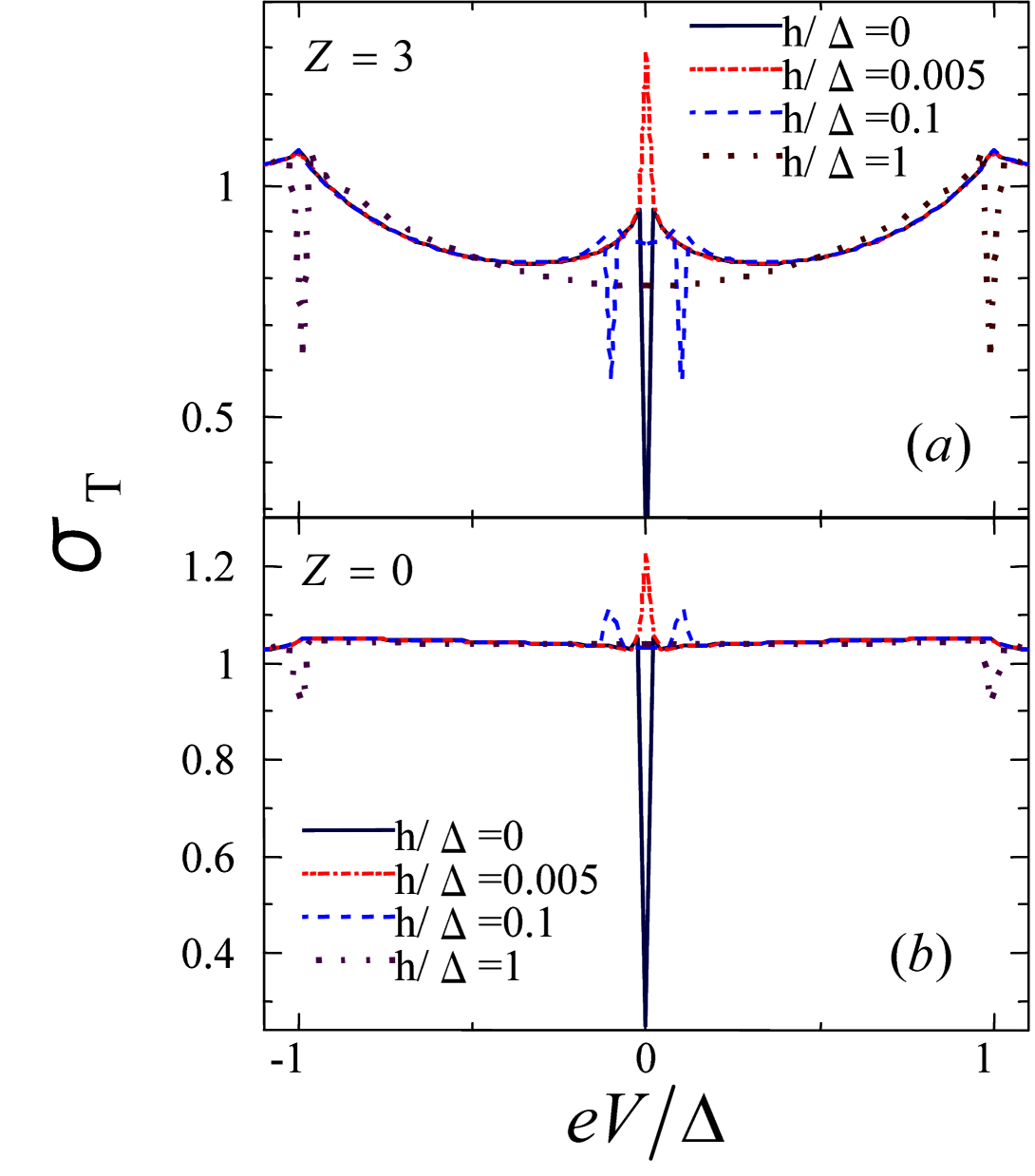
Figure 1: (color online) Normalized tunneling conductance for $s$-wave superconductors with $R_{d}/R_{b}=1$ and $E_{Th}/\Delta=0.01$.

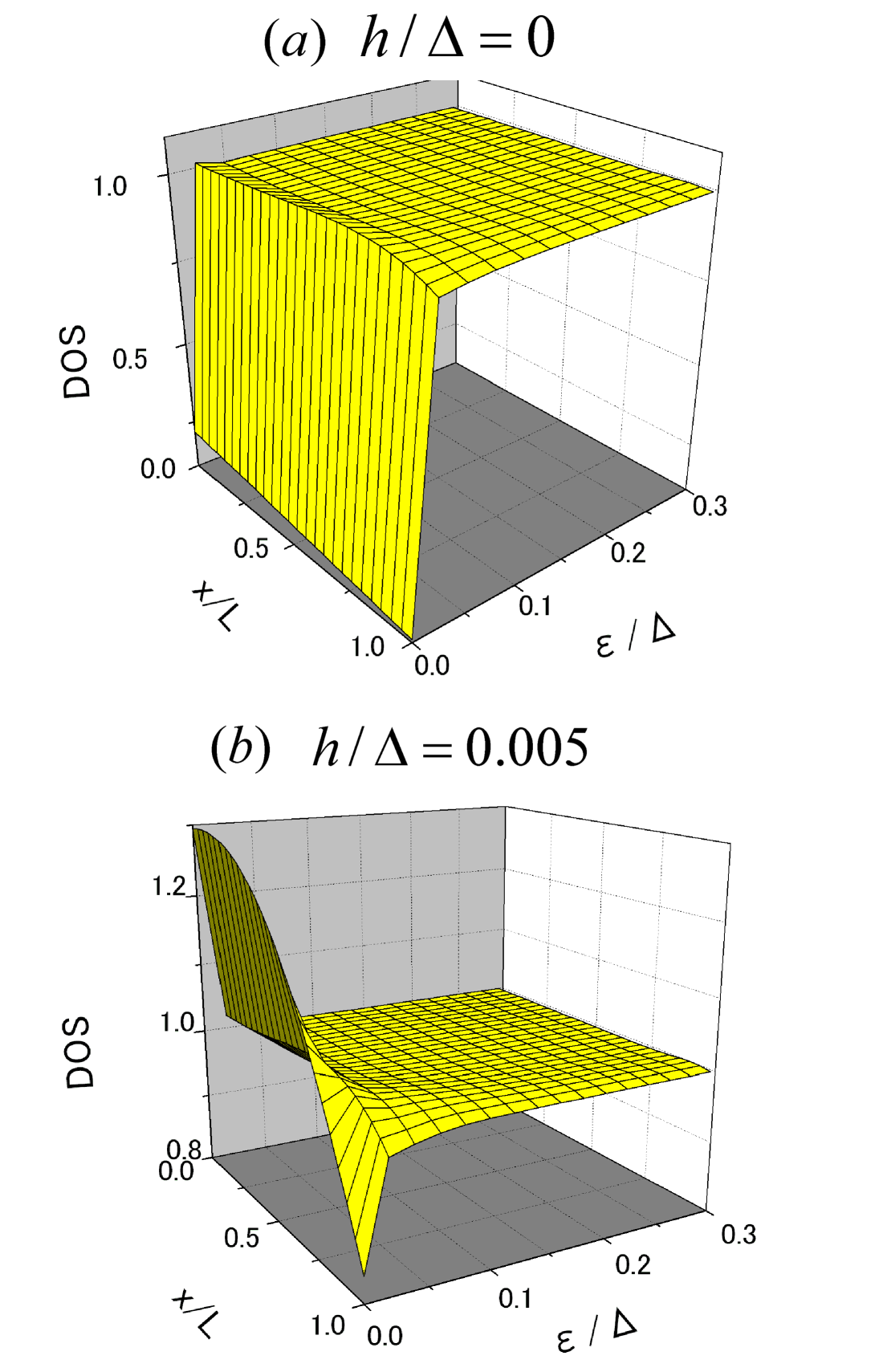
Figure 2: (color online) Normalized DOS for $s$-wave superconductors with $Z=3$, $R_{d}/R_{b}=1$ and $E_{Th}/\Delta=0.01$.

Next we choose the strong proximity regime and relatively small Thouless energy, $E_{Th}/\Delta=0.01$. In the present case, the resonant ZBCP is expected for $h/\Delta=0.01$. Figure 3 displays the tunneling conductance for $R_{d}/R_{b}=5$ and $E_{Th}/\Delta=0.01$ and various $h/\Delta$ with (a) $Z=3$ and (b) $Z=0$. In this case we also find resonant ZBCP and splitting of the peak as in Fig. 1. The corresponding DOS of Fig. 3(a) is shown in Fig. 4 for (a) $h/\Delta=0$ and (b) $h/\Delta=0.01$. For $h=0$, a sharp dip appears at zero energy. For finite energy the DOS is almost unity and spatially independent. For $h/\Delta=0.01$ a peak occurs at zero energy in the range of $x$ near the DF/N interface. We can find similar structures in the corresponding conductance as shown in Fig. 3. The DOS around zero energy is strongly suppressed at the DF/S interface $(x=L)$ compared to the one in Fig. 2.

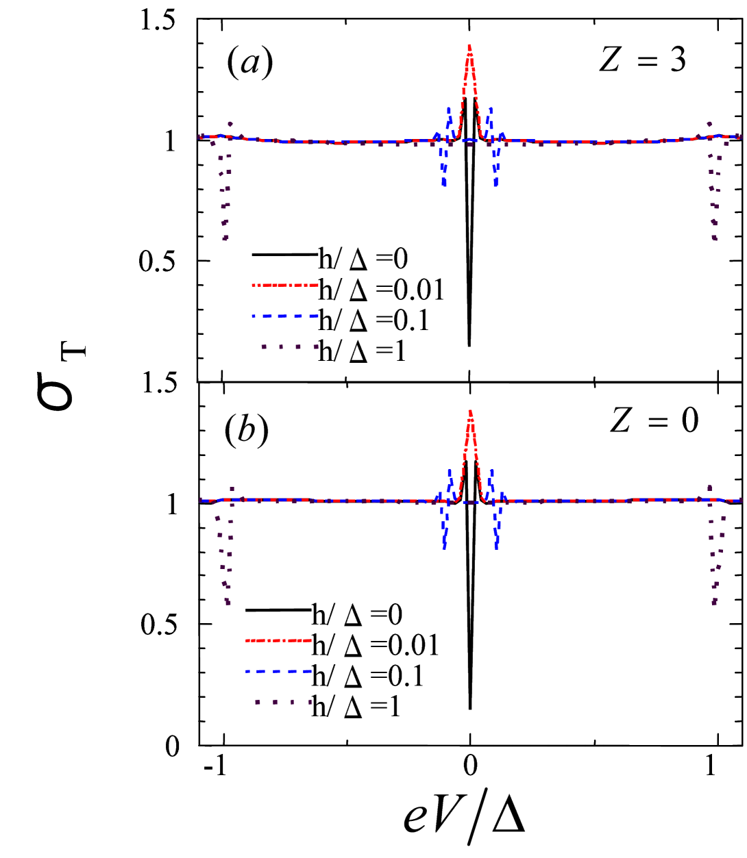
Figure 3: (color online) Normalized tunneling conductance for $s$-wave superconductors with $R_{d}/R_{b}=5$ and $E_{Th}/\Delta=0.01$.

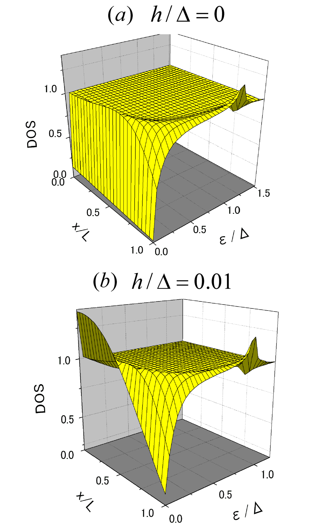
Figure 4: (color online) Normalized DOS for $s$-wave superconductors with $Z=3$, $R_{d}/R_{b}=5$ and $E_{Th}/\Delta=0.01$.

Let us study the junctions with relatively large Thouless energy. In this case, tunneling conductance is insensitive to the change of $Z$. In Fig. 5 we show the tunneling conductance and corresponding DOS for $Z=3$, $R_{d}/R_{b}=1$, $E_{Th}/\Delta=10$ and various $h/\Delta$. We find the broad peak of the conductance by the resonant proximity effect for $h/\Delta=5$ in Fig. 5 (a). For $h/\Delta=0$, the DOS has a gap-like structure as shown in Fig. 5 (b) while for $h/\Delta=5$ it has a zero-energy peak as shown in Fig. 5 (c). Similar plots are shown in Fig. 6 for $Z=3$, $R_{d}/R_{b}=5$, $E_{Th}/\Delta=10$ and various $h/\Delta$. We find the broad ZBCP by the resonant proximity effect for $h/\Delta=10$ in Fig. 6 (a). The DOS for $h/\Delta=0$ has a gap-like structure as shown in Fig. 6 (b). For $h/\Delta=10$ a zero-energy peak appears as shown in Fig. 6 (c).

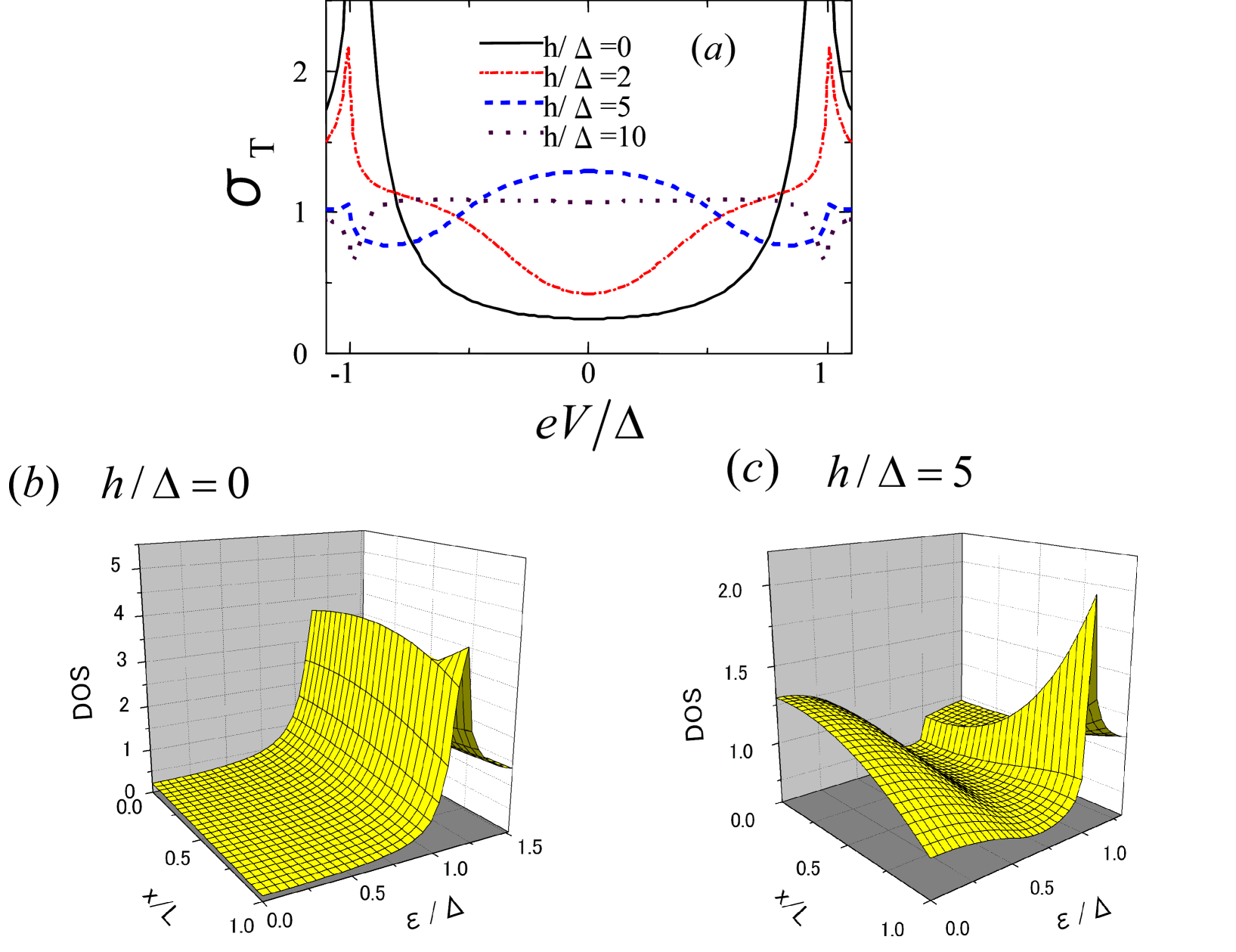
Figure 5: (color online) Normalized tunneling conductance and corresponding DOS for $s$-wave superconductors with $Z=3$, $R_{d}/R_{b}=1$ and $E_{Th}/\Delta=10$.

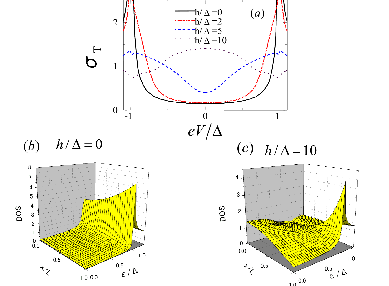
Figure 6: (color online) Normalized tunneling conductance and corresponding DOS for $s$-wave superconductors with $Z=3$, $R_{d}/R_{b}=5$ and $E_{Th}/\Delta=10$.

Before ending this subsection we will look at the spatial dependence of the proximity parameter, $\theta$. Figure 7 displays the spatial dependence of Re$\theta$ and Im$\theta$ for majority spin at zero energy. We choose the same parameters as those in Fig 1 (a) and Fig 3 (a) for (a), (b) and (c), (d) in Fig. 7 respectively. For the appearance of the DOS peak, large value of Im$\theta$ is needed because the normalized DOS is given by Re$\cos(\theta)=\cos(Re(\theta))\cosh(Im(\theta))$. When the resonant conditions are satisfied, Im$\theta$ has an actually large value as shown in Fig. 7 (b) and (d). Otherwise we can see the damped oscillating behavior of the proximity parameter. In contrast to Im$\theta$, Re$\theta$ becomes suppressed with increasing $h/\Delta$ independently of the resonant proximity effect (Fig. 7 (a) and (c)).

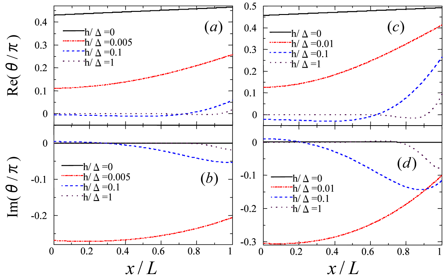
Figure 7: (color online) Spatial dependence of Re$\theta$ and Im$\theta$ for $s$-wave superconductors with $Z=3$, $E_{Th}/\Delta=0.01$. $R_{d}/R_{b}=1$ (left panels) and $R_{d}/R_{b}=5$ (right panels).

III.2 Junctions with $d$-wave superconductors

In this subsection, we focus on the $d$-wave junctions both for weak and strong proximity regimes. In this case, depending on the orientation angle $\alpha$, the proximity effect is drastically changed: as $\alpha$ increases the proximity effect is suppressedNazarov3 ; Golubov2 . For $\alpha=0$ we can expect similar results to the $s$-wave junctions since proximity effect exists while the MARS is absent. On the other hand, the tunneling conductance for large $\alpha$ is almost independent of $h/\Delta$. Especially, the conductance is independent of $h$ for $\alpha/\pi=0.25$ due to the complete absence of the proximity effect. Two different mechanisms of formation of ZBCP exist in DF/D junctions: the ZBCP caused by the resonant proximity effect peculiar to a ferromagnet and the ZBCP caused by the MARS located at DF/D interface. When $\alpha$ increases, MARS are formed and at the same time the proximity effect becomes weakened. Therefore the MARS provide the dominant contribution to the ZBCP compared to the resonant proximity effect, as will be discussed below.

First we choose the weak proximity regime where the resonant condition is $h/\Delta=0.005$. Figure 8 displays the tunneling conductance for $Z=3$, $R_{d}/R_{b}=1$ and various $\alpha$ with (a) $E_{Th}/\Delta=0.01$ and $h/\Delta=0$, (b) $E_{Th}/\Delta=0.01$ and $h/\Delta=0.005$, (c) $E_{Th}/\Delta=10$ and $h/\Delta=0$, and (d) $E_{Th}/\Delta=10$ and $h/\Delta=5$. For $E_{Th}/\Delta=0.01$ and $h=0$ ZBCD appears for $\alpha/\pi=0$ due to the proximity effect as in the case of the $s$-wave junctions while ZBCP appears for $\alpha/\pi=0.25$ due to the formation of the MARS (Fig. 8 (a)). For $E_{Th}/\Delta=0.01$ and $h/\Delta=0.005$, the height of the ZBCP by the resonant proximity effect exceeds the one by MARS for $\alpha/\pi=0.25$ (Fig. 8 (b)). Since in the ballistic junctions, the ZBCP for $\alpha/\pi=0.25$ is most strongly enhancedTK95 ; Kashi00 ; Experiments , this ZBCP by the resonant proximity effect in DF is a remarkable feature. Such a feature is also expected for a larger magnitude of $E_{Th}$. For $E_{Th}/\Delta=10$ and $h=0$, a V-like shape of the conductance appears for $\alpha/\pi=0$ while ZBCP appears for $\alpha/\pi=0.25$ (Fig. 8 (c)). In this case, by choosing $h/\Delta=5$, a broad peak by the resonant proximity effect appears for $\alpha/\pi=0$ and its height exceeds the one for $\alpha/\pi=0.25$ (Fig. 8 (d)).

We also study the DOS of the DF for the same parameters as those in Fig. 8 (d) with (a) $\alpha/\pi=0$ and (b) $\alpha/\pi=0.125$ in Fig. 9. For $\alpha/\pi=0$ a zero-energy peak appears as in the case of $s$-wave junctions. With increasing $\alpha$ the DOS around zero energy becomes suppressed due to the reduction of the proximity effect. The extreme case is $\alpha/\pi=0.25$, where the DOS is always unity since the proximity effect is completely absent.

Next we consider the junctions in the strong proximity regime. Figure 10 shows the tunneling conductance for $Z=3$, $R_{d}/R_{b}=5$ and various $\alpha$ with (a) $E_{Th}/\Delta=0.01$ and $h/\Delta=0$, (b) $E_{Th}/\Delta=0.01$ and $h/\Delta=0.01$, (c) $E_{Th}/\Delta=10$ and $h/\Delta=0$ and (d) $E_{Th}/\Delta=10$ and $h/\Delta=10$. In this case we also find the ZBCP for $\alpha=0$ caused by the resonant proximity effect. This ZBCP becomes suppressed as $\alpha$ increases, as shown in Figs. 10(b) and (d).

The corresponding DOS of the DF for Fig. 10(d) is shown in Fig. 11. The line shapes of the LDOS at $x=0$ are qualitatively similar to the tunneling conductance. The DOS at the DF/S interface ($x=L$) is drastically suppressed as compared to the one in Fig. 9.

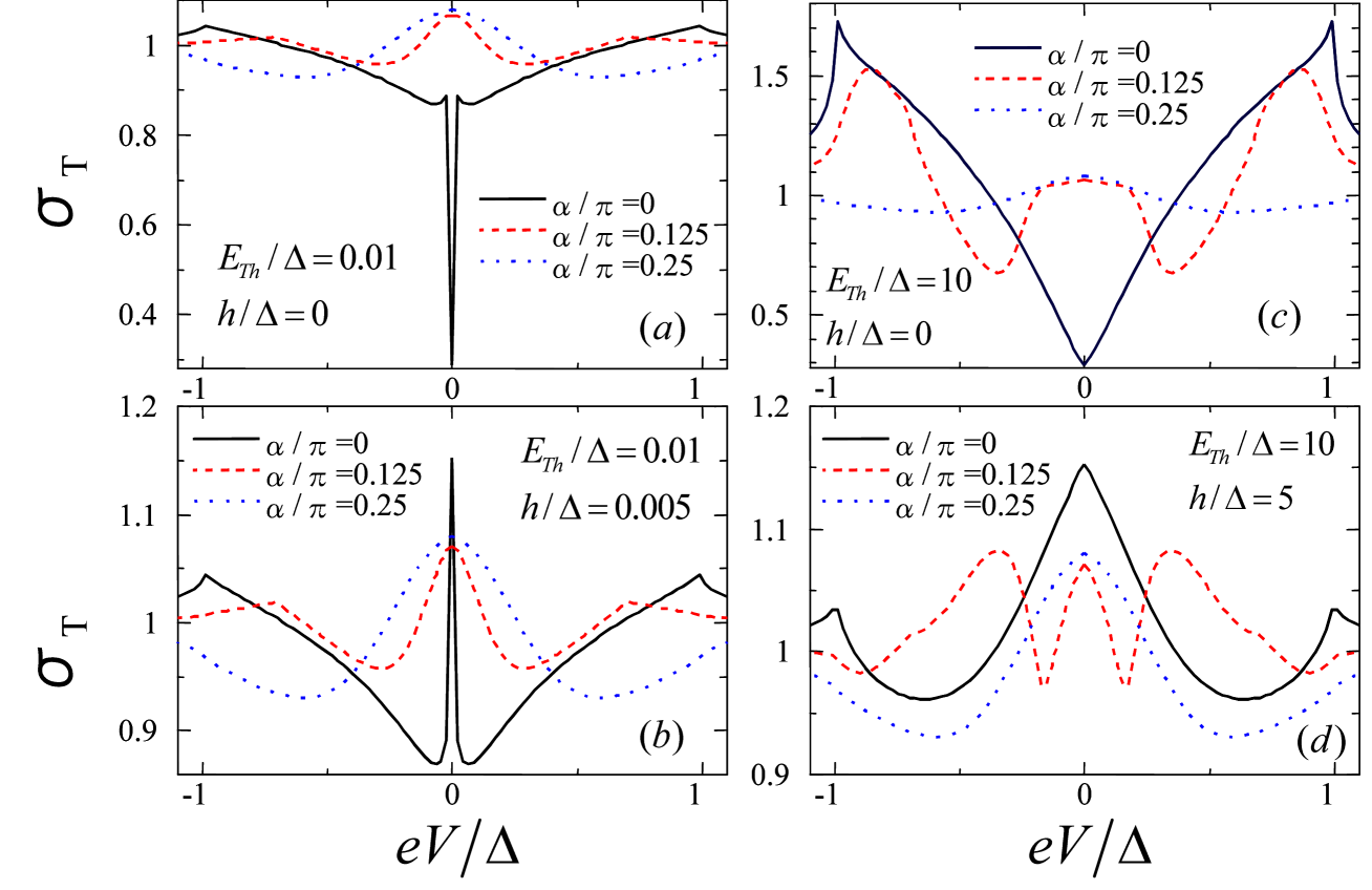
Figure 8: (color online) Normalized tunneling conductance for $d$-wave superconductors with $Z=3$ and $R_{d}/R_{b}=1$.

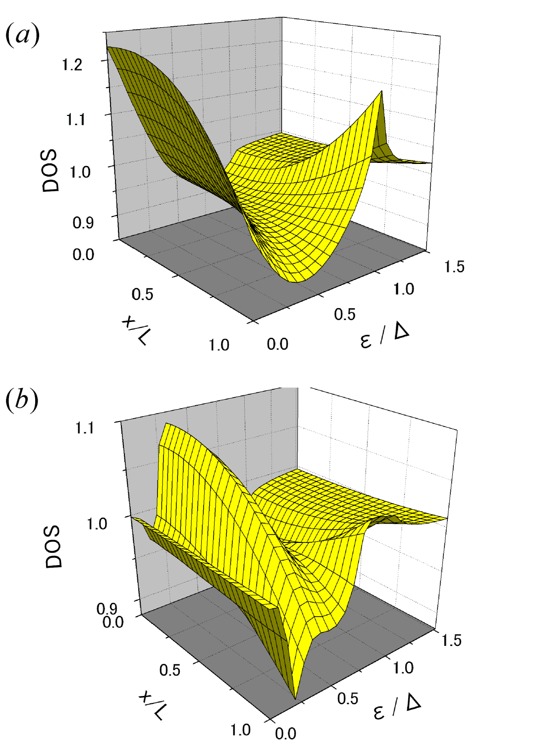
Figure 9: (color online) Normalized DOS for $d$-wave superconductors with $Z=3$, $R_{d}/R_{b}=1$, $E_{Th}/\Delta=10$ and $h/\Delta=5$. (a) $\alpha/\pi=0$ and (b)$\alpha/\pi=0.125$.

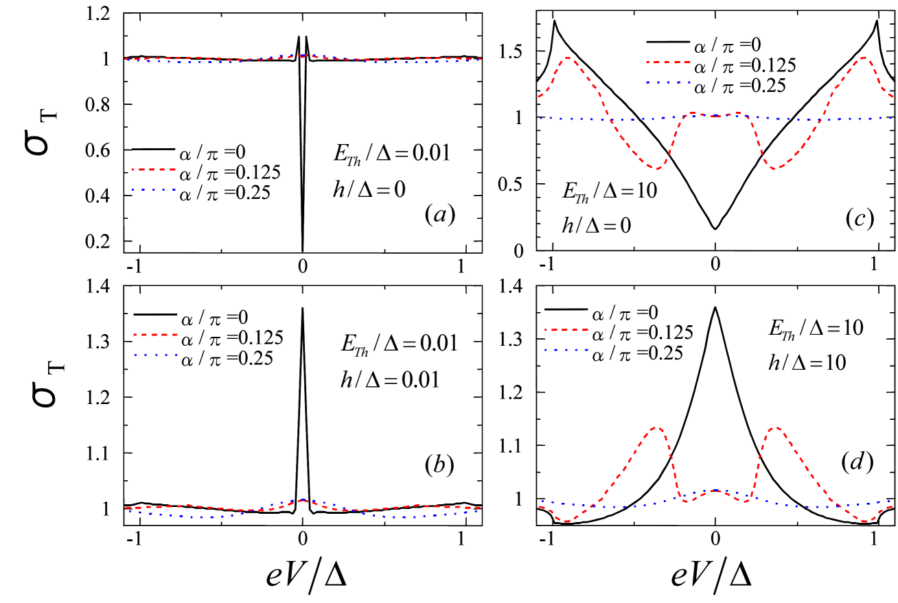
Figure 10: (color online) Normalized tunneling conductance for $d$-wave superconductors with $Z=3$ and $R_{d}/R_{b}=5$.

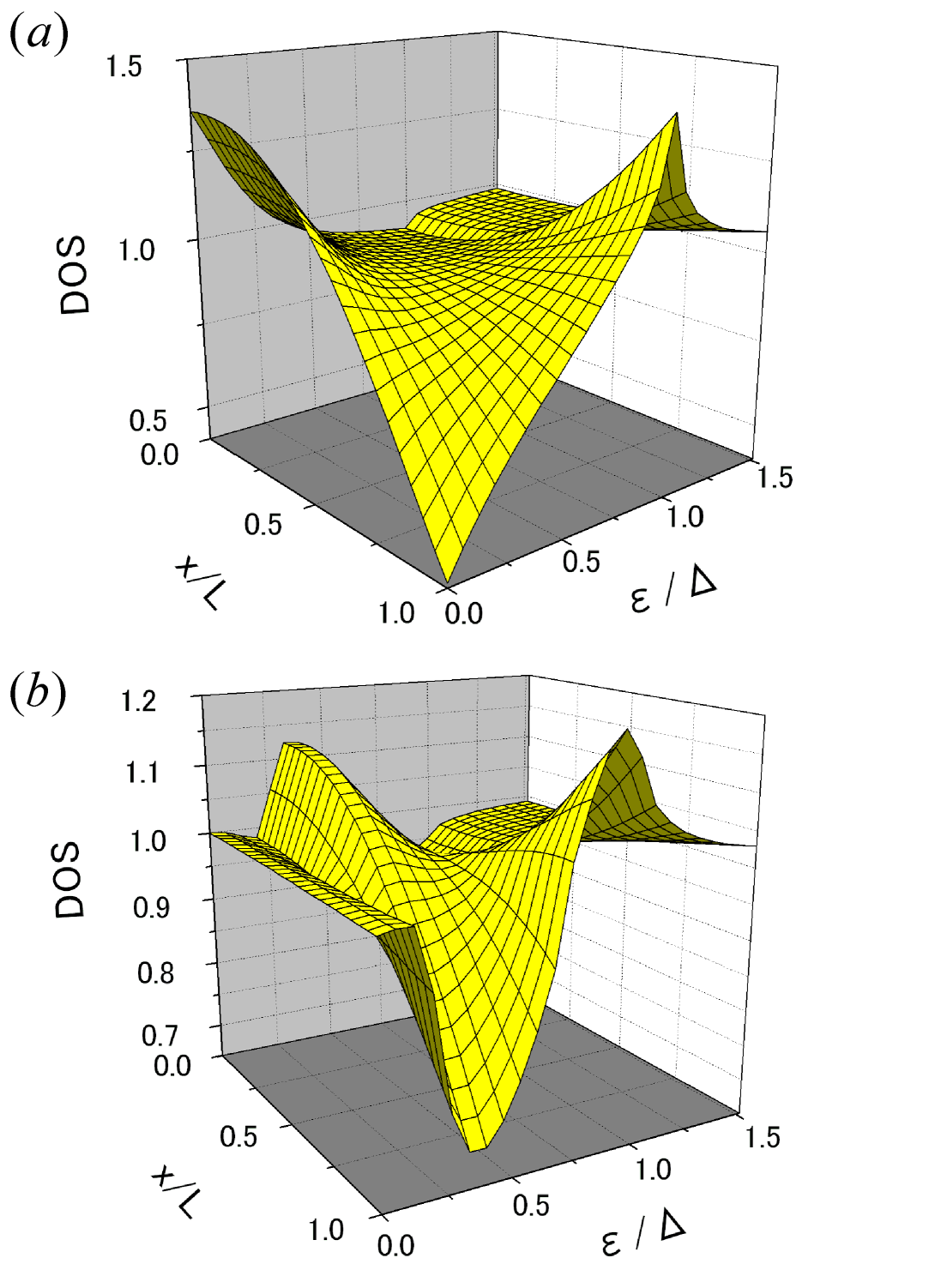
Figure 11: (color online) Normalized DOS for $d$-wave superconductors with $Z=3$, $R_{d}/R_{b}=5$, $E_{Th}/\Delta=10$ and $h/\Delta=10$. (a) $\alpha/\pi=0$ and (b)$\alpha/\pi=0.125$.

IV Conclusions

In the present paper, a detailed theoretical study of the tunneling conductance and the density of states in normal metal / diffusive ferromagnet / $s$- and $d$-wave superconductor junctions is presented. We have clarified that the resonant proximity effect strongly influences the tunneling conductance and the density of states. There are several points which have been clarified in this paper.

1. For $s$-wave junctions, due to the resonant proximity effect, a sharp ZBCP appears for small $E_{Th}$ while a broad ZBCP appears for large $E_{Th}$ . We have shown that the mechanism of the ZBCP in DF/S junctions is essentially different from that in DN/S junctions and is due to the strong enhancement of DOS at a certain value of the exchange field. As a result, the magnitude of ZBCP in DF/S can exceed its normal state value in contrast to the case of DN/S junctions.

2. For $d$-wave junctions at $\alpha=0$, similar to the s-wave case, the sharp ZBCP is formed when the resonant condition is satisfied. At finite misorientation angle $\alpha$, the MARS contribute to the conductance when $R_{d}/R_{b}\ll 1$ and $Z\gg 1$. With the increase of $\alpha$ the contribution of the resonant proximity effect becomes smaller while the MARS dominate the conductance. As a result, for sufficiently large $\alpha$ ZBCP exists independently of whether the resonant condition is satisfied or not. In the opposite case of the weak barrier, $R_{d}/R_{b}\gg 1$, the contribution of MARS is negligible and ZBCP appears only when the resonant condition is satisfied.

An interesting problem is a calculation of the tunneling conductance in normal metal / diffusive ferromagnet / $p$-wave superconductor junctions because interesting phenomena were predicted in diffusive normal metal / $p$-wave superconductor junctionsp-wave . We will address this problem in a separate study.

The authors appreciate useful and fruitful discussions with J. Inoue, Yu. Nazarov and H. Itoh. This work was supported by NAREGI Nanoscience Project, the Ministry of Education, Culture, Sports, Science and Technology, Japan, the Core Research for Evolutional Science and Technology (CREST) of the Japan Science and Technology Corporation (JST) and a Grant-in-Aid for the 21st Century COE ”Frontiers of Computational Science” . The computational aspect of this work has been performed at the Research Center for Computational Science, Okazaki National Research Institutes and the facilities of the Supercomputer Center, Institute for Solid State Physics, University of Tokyo and the Computer Center.

References

- (1) A.F. Andreev, Sov. Phys. JETP 19, 1228 (1964).
- (2) G.E. Blonder, M. Tinkham, and T.M. Klapwijk, Phys. Rev. B 25, 4515 (1982).
- (3) P. M. Tedrow and R. Meservey, Phys. Rev. Lett. 26, 192 (1971); Phys. Rev. B 7, 318 (1973); R. Meservey and P. M. Tedrow, Phys. Rep. 238, 173 (1994).
- (4) S. K. Upadhyay, A. Palanisami, R. N. Louie, and R. A. Buhrman Phys. Rev. Lett. 81, 3247 (1998).
- (5) R. J. Soulen Jr., J. M. Byers, M. S. Osofsky, B. Nadgorny, T. Ambrose, S. F. Cheng, P. R. Broussard, C. T. Tanaka, J. Nowak, J. S. Moodera, A. Barry, J. M. D. Coey Science 282, 85 (1998)
- (6) I.I.Mazin, A.A.Golubov, and B.Nadgorny J.Appl.Phys. 89, 7576 (2001).
- (7) G.T. Woods, R. J. Soulen, I. I. Mazin, B. Nadgorny, M. S. Osofsky, J. Sanders, H. Srikanth, W. F. Egelhoff, and R. Datla, Phys. Rev. B 70, 054416 (2004).
- (8) W. Belzig, A. Brataas, Yu. V. Nazarov, G. E. W. Bauer, Phys. Rev. B 62, 9726 (2000).
- (9) T. Hirai, Y. Tanaka, N. Yoshida, Y. Asano, J. Inoue, and S. Kashiwaya Phys. Rev. B 67, 174501 (2003); N. Yoshida, Y. Tanaka, J. Inoue, and S. Kashiwaya, J. Phys. Soc. Jpn. 68, 1071 (1999); S. Kashiwaya, Y. Tanaka, N. Yoshida, and M.R. Beasley, Phys. Rev. B 60, 3572 (1999); I. Zutic and O.T. Valls, Phys. Rev. B 60, 6320 (1999); 61, 1555 (2000); N. Stefanakis, Phys. Rev. B 64, 224502 (2001); J. Phys. Condens. Matter 13, 3643 (2001).
- (10) A.I. Buzdin, L.N. Bulaevskii, and S.V. Panyukov, Pis’ma Zh. Eksp. Teor. Phys. 35, 147, (1982) [JETP Lett. 35, 178 (1982)].
- (11) A.I. Buzdin and M.Yu. Kupriyanov, Pis’ma Zh. Eksp. Teor. Phys. 53, 308 (1991) [JETP Lett. 53, 321 (1991)].
- (12) E. A. Demler, G. B. Arnold, and M. R. Beasley, Phys. Rev. B 55, 15 174 (1997).
- (13) A. I. Buzdin, Rev. Mod. Phys. 77, 935 (2005).
- (14) A. A. Golubov, M. Yu. Kupriyanov, and E. Il’ichev, Rev. Mod. Phys. 76, 411 (2004).
- (15) F. S. Bergeret, A. F. Volkov, and K. B. Efetov, cond-mat/0506047, Rev. Mod. Phys. 77, xxx (2005).
- (16) V. V. Ryazanov, V. A. Oboznov, A. Yu. Rusanov, A. V. Veretennikov, A. A. Golubov, and J. Aarts, Phys. Rev. Lett. 86, 2427 (2001); V. V. Ryazanov, V. A. Oboznov, A. V. Veretennikov, and A. Yu. Rusanov, Phys. Rev. B 65, 020501(R) (2001); S. M. Frolov, D. J. Van Harlingen, V. A. Oboznov, V. V. Bolginov, and V. V. Ryazanov, Phys. Rev. B 70, 144505.
- (17) T. Kontos, M. Aprili, J. Lesueur, F. Genet, B. Stephanidis, and R. Boursier, Phys. Rev. Lett. 89, 137007 (2002).
- (18) Y. Blum, A. Tsukernik, M. Karpovski, and A. Palevski, Phys. Rev. Lett. 89, 187004 (2002).
- (19) H. Sellier, C. Baraduc, F. Lefloch, and R. Calemczuk, Phys. Rev. B 68, 054531 (2003).
- (20) A. Bauer, J. Bentner, M. Aprili, M. L. Della-Rocca, M. Reinwald, W. Wegscheider, and C. Strunk, Phys. Rev. Lett. 92, 217001 (2004).
- (21) Z. Radovic, M. Ledvij, Lj. Dobrosavljevic-Grujic, A. I. Buzdin, and J. R. Clem, Phys. Rev. B 44, 759 (1991).
- (22) L. R. Tagirov, Phys. Rev. Lett. 83, 2058 (1999).
- (23) Ya. V. Fominov, N. M. Chtchelkatchev, and A. A. Golubov, Pis’ma Zh. Eksp. Teor. Fiz. 74, 101 (2001) [JETP Lett. 74, 96 (2001)]; Ya. V. Fominov, N. M. Chtchelkatchev, and A. A. Golubov, Phys. Rev. B 66, 014507 (2002).
- (24) A. Rusanov, R. Boogaard, M. Hesselberth, H. Sellier, and J. Aarts, Physica C 369, 300 (2002).
- (25) V.V.Ryazanov, V.A.Oboznov, A.S.Prokofiev, S.V.Dubonos, JETP Lett. 77, 39 (2003).
- (26) A. Kadigrobov, R. I. Shekhter, M. Jonson and Z. G. Ivanov, Phys. Rev. B 60, 14593 (1999).
- (27) R. Seviour, C. J. Lambert, and A. F. Volkov , Phys. Rev. B 59, 6031 (1999).
- (28) M. Leadbeater, C. J. Lambert, K. E. Nagaev, R. Raimondi and A. F. Volkov, Phys. Rev. B 59, 12264 (1999).
- (29) F. S. Bergeret, K. B. Efetov, and A. I. Larkin, Phys. Rev. B 62, 11872 (2000); F. S. Bergeret, A. F. Volkov, and K. B. Efetov, Phys. Rev. Lett. 86, 4096 (2001).
- (30) A. Kadigrobov, R. I. Shekhter, and M. Jonson, Europhys. Lett. 54, 394 (2001).
- (31) A. Buzdin, Phys. Rev. B 62, 11 377 (2000).
- (32) M. Zareyan, W. Belzig, and Yu. V. Nazarov, Phys. Rev. Lett. 86, 308 (2001); Phys. Rev. B 65, 184505 (2002).
- (33) I. Baladie and A. Buzdin, Phys. Rev. B 64, 224514 (2001).
- (34) F. S. Bergeret, A. F. Volkov, and K. B. Efetov, Phys. Rev. B 65, 134505 (2002).
- (35) A. A. Golubov, M. Yu. Kupriyanov, and Ya. V. Fominov, JETP Lett. 75, 223 (2002).
- (36) V. N. Krivoruchko and E. A. Koshina, Phys. Rev. B 66, 014521 (2002).
- (37) T. Kontos, M. Aprili, J. Lesueur, and X. Grison, Phys. Rev. Lett. 86, 304 (2001); T. Kontos, M. Aprili, J. Lesueur, X. Grison, and L. Dumoulin, Phys. Rev. Lett. 93, 137001 (2004).
- (38) T. Yokoyama, Y. Tanaka, and A. A. Golubov, Phys. Rev. B 72, 052512 (2005).
- (39) L.J. Buchholtz and G. Zwicknagl, Phys. Rev. B 23 5788 (1981); C. Bruder, Phys. Rev. B 41, 4017 (1990); C.R. Hu, Phys. Rev. Lett. 72, 1526 (1994).
- (40) Y. Tanaka and S. Kashiwaya, Phys. Rev. Lett. 74, 3451 (1995); S. Kashiwaya, Y. Tanaka, M. Koyanagi and K. Kajimura, Phys. Rev. B 53, 2667 (1996); Y. Tanuma, Y. Tanaka, and S. Kashiwaya Phys. Rev. B 64, 214519 (2001).
- (41) S. Kashiwaya and Y. Tanaka, Rep. Prog. Phys. 63, 1641 (2000) and references therein.
- (42) J. Geerk, X.X. Xi, and G. Linker: Z. Phys. B. 73,(1988) 329; S. Kashiwaya, Y. Tanaka, M. Koyanagi, H. Takashima, and K. Kajimura, Phys. Rev. B 51 1350 (1995); L. Alff, H. Takashima, S. Kashiwaya, N. Terada, H. Ihara, Y. Tanaka, M. Koyanagi, and K. Kajimura, Phys. Rev. B 55, 14757 (1997); M. Covington, M. Aprili, E. Paraoanu, L.H. Greene, F. Xu, J. Zhu, and C.A. Mirkin, Phys. Rev. Lett. 79, 277 (1997); J. Y. T. Wei, N.-C. Yeh, D. F. Garrigus and M. Strasik: Phys. Rev. Lett. 81, (1998) 2542; I. Iguchi, W. Wang, M. Yamazaki, Y. Tanaka, and S. Kashiwaya: Phys. Rev. B 62, (2000) R6131; F. Laube, G. Goll, H.v. Löhneysen, M. Fogelström, and F. Lichtenberg, Phys. Rev. Lett. 84, 1595 (2000); Z.Q. Mao, K.D. Nelson, R. Jin, Y. Liu, and Y. Maeno, Phys. Rev. Lett. 87, 037003 (2001); Ch. Wälti, H.R. Ott, Z. Fisk, and J.L. Smith, Phys. Rev. Lett. 84, 5616 (2000); H. Aubin, L. H. Greene, Sha Jian and D. G. Hinks, Phys. Rev. Lett. 89, 177001 (2002); Z. Q. Mao, M. M. Rosario, K. D. Nelson, K. Wu, I. G. Deac, P. Schiffer, Y. Liu, T. He, K. A. Regan, and R. J. Cava Phys. Rev. B 67 , 094502 (2003); A. Sharoni, O. Millo, A. Kohen, Y. Dagan, R. Beck, G. Deutscher, and G. Koren Phys. Rev. B 65, 134526 (2002); A. Kohen, G. Leibovitch, and G. Deutscher Phys. Rev. Lett. 90, 207005 (2003).
- (43) K.D. Usadel Phys. Rev. Lett. 25, 507 (1970).
- (44) M.Yu. Kupriyanov and V. F. Lukichev, Zh. Exp. Teor. Fiz. 94 (1988) 139 [Sov. Phys. JETP 67, (1988) 1163].
- (45) Yu. V. Nazarov, Superlattices and Microstructuctures 25, 1221 (1999), cond-mat/9811155.
- (46) Y. Tanaka, A. A. Golubov and S. Kashiwaya, Phys. Rev. B 68 054513 (2003).
- (47) Y. Tanaka, Y.V. Nazarov and S. Kashiwaya, Phys. Rev. Lett. 90 167003 (2003).
- (48) Y. Tanaka, Y. V. Nazarov, A. A. Golubov and S. Kashiwaya, Phys. Rev. B 69 144519 (2004).
- (49) Y. Tanaka and S. Kashiwaya, Phys. Rev. B 70 012507 (2004); Y. Tanaka, S. Kashiwaya, and T. Yokoyama, Phys. Rev. B 71, 094513 (2005); Y. Tanaka,Y. Asano, A. A. Golubov, and S. Kashiwaya, Phys. Rev. B, in press (2005).
- (50) A.F. Volkov, A.V. Zaitsev and T.M. Klapwijk, Physica C 210, 21 (1993).
- (51) A. Kastalsky, A.W. Kleinsasser, L.H. Greene, R. Bhat, F.P. Milliken, J.P. Harbison, Phys. Rev. Lett. 67, 3026 (1991).