Non-equilibrium spin polarization effect in spin-orbit coupling system and contacting leads

Abstract

We study theoretically the current-induced spin polarization effect in a two-terminal mesoscopic structure which is composed of a semiconductor two-dimensional electron gas (2DEG) bar with Rashba spin-orbit (SO) interaction and two attached ideal leads. The nonequilibrium spin density is calculated by solving the scattering wave functions explicitly within the ballistic transport regime. We found that for a Rashba SO system the electrical current can induce spin polarization in the SO system as well as in the ideal leads. The induced polarization in the 2DEG shows some qualitative features of the intrinsic spin Hall effect. On the other hand, the nonequilibrium spin density in the ideal leads, after being averaged in the transversal direction, is independent of the distance measured from the lead/SO system interface, except in the vicinity of the interface. Such a lead polarization effect can even be enhanced by the presence of weak impurity scattering in the SO system and may be detectable in real experiments.

I Introduction

Recently there has been hot research interest in spin-polarized transport phenomena in semiconductor systems with spin-orbit ( SO ) coupling because of their potential applications in the field of semiconductor spintronicsWolf2001 ; semibook2002 ; Dassarma2004 . One of the principal challenges in semiconductor spintronics is the efficient injection and effective manipulation of non-equilibrium spin densities and/or spin currents in nonmagnetic semiconductors by electric means, and within this context, the recently predicted phenomenon of intrinsic spin Hall effect would be much attractive. This phenomenon was conceived to survive in some semiconductor systems with intrinsic spin-orbit interactions and it consists of a spin current contribution in the direction perpendicular to a driving charge current circulating through a sample. This phenomenon was firstly proposed to survive in p-doped bulk semiconductors with spin-orbit split band structures by Murakami et al.MurakamiScience2003 and in two-dimensional electronic systems with Rashba spin-orbit coupling by Sinova et al..SinovaPRL2004 In the last two years lots of theoretical work have been devoted to the study of this phenomenon and intensive debates arose on some fundamental issues concerning this effect. JPHu2003 ; RashbaPRB2003 ; SQShen2004 ; InouePRB2004 ; MishchenkoPRL2004 ; RashbaPRB2004 ; LShengPRL2005 ; MurakamiPRB2004 ; Bernevig2004 ; Nikolic2004 ; Nikolic2005 ; yqli ; PZhang2005 ; BernevigB2004 ; DNSheng2005 Now it was well established that this effect should be robust against impurity scattering in a mesoscopic semiconductor system with intrinsic spin-orbit coupling, but it cannot survive in a diffusive two-dimensional electron gas with k-linear intrinsic spin-orbit coupling due to vertex correction from impurity scattering.InouePRB2004 ; MishchenkoPRL2004 ; RashbaPRB2004 ; DNSheng2005 . It also should be noted that, prior to the prediction of this effect, a similar phenomenon called extrinsic spin Hall effect had also been predicted by Dyakanov-PerelMD and HirschHirsch99 ; Zhang00 . Unlike the intrinsic spin Hall effect, the extrinsic spin Hall effect arises from spin-orbit dependent impurity scattering and hence it is a much weak effect compared with the intrinsic spin Hall effect, and especially, it will disappear completely in the absence of spin-orbit dependent impurity scattering.

A physical quantity which is intuitively a direct consequence of a spin Hall effect in a semiconductor strip is the nonequilibrium spin accumulation near the transversal boundaries of the strip when a longitudinal charge current circulates through it. The recent experimental observations in n-doped bulk GaAsKatoScience2004 and in p-doped two-dimensional GaAsWunderlichPRL2005 have revealed the possibility of generating non-equilibrium edge spin accumulation in a semiconductor strip by an extrinsicKatoScience2004 or intrinsicWunderlichPRL2005 spin Hall effect, though from the theoretical points of view some significant controversies may still exist for the detailed theoretical interpretations of some experimental data.BernevigB2004 ; Nikolic2004 ; Usaj2005 ; Zyang2005 ; jianghu1 . It also should be noticed that, in addition to the spin Hall effect, there may be some other physical reasons that may lead to the generation of electric-current-induced spin polarization in a spin-orbit coupled system. For example, the experimental results reported in RefSilov had demonstrated another kind of electric-current-induced spin polarization effect in a spin-orbit coupled system, which can be interpreted as the inverse of the photogalvanic effectSilov . In the present paper we are interested in the question that, besides the transverse boundary spin accumulations, what kinds of other physical consequences can be predicted for a semiconductor strip with intrinsic SO coupling. To be specific, we will consider a strip of a mesoscopic two-dimensional electron gas with Rashba spin-orbit coupling connected to two ideal leads. For such a system, we show that when a longitudinal charge current circulates through the strip, besides the transverse boundary spin accumulations in the strip, non-equilibrium spin polarizations can also be induced in the leads, and the non-equilibrium spin polarizations in the leads will also depend sensitively on the spin-orbit coupling parameters in the strip. Furthermore we will show that in the absence of spin-orbit coupling in the leads, the non-equilibrium spin polarizations in the leads will be independent of the distance away from the border between the lead and the strip, except in the vicinity of the border where local states play an important role. The signs and the amplitudes of the non-equilibrium spin polarization in the leads is adjustable by switching the charge current direction and by tuning the Rashba SO coupling strength in the strip. Furthermore, in the presence of weak disorder inside the SO strip, the spin polarization effect in the leads can be even enhanced while spin polarization in the strip is decreased, so such an effect might be more easily detectable than the spin polarization inside the strip. The non-equilibrium lead polarization effect provides a new possibility of all-electric control on spin degree of freedom in semiconductor and thus have practical application potential.

The paper will be organized as following: In section II the model Hamiltonian and the theoretical formalism used in the calculations will be introduced. In section III some symmetry properties and numerical results about the non-equilibrium spin polarizations both in the strip and in the leads will be presented and discussed. At last, we summarize main points of the paper in section IV.

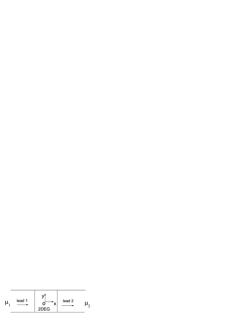
Figure 1: schematic geometry of multi-terminal setup.

II Method of solving scattering wave function and multi-terminal scattering matrix

The system that we will consider in the present paper is depicted in Fig. 1, which consists of a strip of a mesoscopic Rashba two-dimensional electron gas connected to two half-infinite ideal leads. Each lead is connected to an electron reservoir at infinity which has a fixed chemical potential. In the tight binding representation, the Hamiltonian for the total system reads:

$$H=-t\sum_{p}\sum_{<i,j>\sigma}(C_{p_{i}\sigma}^{{\dagger}}C_{p_{j}\sigma}+h.c.)+\sum_{R_{i},\sigma}w_{R_{i}}C_{R_{i}\sigma}^{{\dagger}}C_{R_{i}\sigma}$$ (1)

$$-t\sum_{<R_{i},R_{j}>\sigma}(C_{R_{i}\sigma}^{{\dagger}}C_{R_{j}\sigma}+h.c.)$$

$$-t_{R}\sum_{R_{i}}[i(\Psi_{R_{i}}^{{\dagger}}\sigma^{x}\Psi_{R_{i}+y}-\Psi_{R_{i}}^{{\dagger}}\sigma^{y}\Psi_{R_{i}+x})+h.c.]$$

$$-t\sum_{p_{n},R_{n}}(C_{p_{n}\sigma}^{{\dagger}}C_{R_{n}\sigma}+h.c.)$$

Here $t=\frac{\hbar^{2}}{2m^{\ast}a^{2}}$ is the hopping parameter between two nearest-neighbor sites where $m^{\ast}$ is effective mass of electrons and $a$ the lattice constant in the 2DEG bar. $\Psi_{R_{i}}^{{\dagger}}=(C_{R_{i},\uparrow},C_{R_{i},\downarrow})$ is the spinor vector for the site $R_{i}$ ( $R_{i}=(x,y)$) in the Rashba SO system. $\sigma^{x},\sigma^{y}$ are the standard pauli matrices. $C_{p_{j}\sigma}$ is the annihilation operator for the site $p_{j}$ with spin $\sigma$ in lead p. $p_{n}$ and $R_{n}$ stand for nearest-neighbor pair on the two sides across the interface of the SO system and the lead $p$. $w_{R_{i}}$ is the on-site energy in the SO system, which can readily incorporate random impurity potential. In a pure system we always set $w_{R_{i}}$ to zero. $t_{R}$ is Rashba coupling coefficient.

Our calculations will follow the same spirit of the usual Landauer-Büttiker’s approach. But unlike the frequently used Green’s function formalismLShengPRL2005 ; JLi2005 , in the formalism used in the present paper we will solve the scattering wave functions in the whole system explicitly. To this end, we firstly consider the scattering wave of an electron incident from a lead. The real space wave function of an incident electron with spin $\sigma$ will be denoted as $e^{-ik_{m}^{p}x_{p}}\chi_{m\sigma}^{p}(y_{p})$, where $\chi_{m\sigma}^{p}(y_{p})$ denotes the $m$’th transverse mode with spin index $\sigma$ in the lead $p$ and $k_{m}^{p}$ the longitudinal wave vector. We adopt the local coordinate scheme for all leads. In the local coordinate scheme, the longitudinal coordinate $x_{q}$ in lead $q$ will take the integer numbers $1,2,$…,$\infty$ away from the 2DEG interface and the transverse coordinate $y_{q}$ take the value of $-N_{q}/2,...,N_{q}/2$. The longitudinal wave vector $k_{m}^{p}$ satisfies the relation $-2t\cos(k_{m}^{p})+\varepsilon_{m}^{p}=E$, where $\varepsilon_{m}^{p}$ is the eigen-energy of the $m$’th transverse mode in lead $p$ and $E$ the energy of the incident electron. Including both the incident and reflected waves, the total wave function in the lead $q$ has the the following general form:

$$\psi_{\sigma\prime}^{pm\sigma}(x_{q},y_{q}) = \delta_{pq}\delta_{\sigma\sigma\prime}e^{-ik_{m}^{p}x_{p}}\chi_{m\sigma}^{p}(y_{p})$$ (2)

$$+\sum_{n\in{q}}\phi_{qn\sigma^{\prime}}^{pm\sigma}e^{ik_{n}^{q}x_{q}}\chi_{n\sigma^{\prime}}^{q}(y_{q})$$

where $\phi_{qn\sigma^{\prime}}^{pm\sigma}$ stands for the scattering amplitude from the ($m\sigma$) mode in lead $p$ to the ($n\sigma^{\prime}$) mode in lead $q$. The scattering amplitudes $\phi_{qn\sigma^{\prime}}^{pm\sigma}$ will be determined by solving the Schrödinger equation for the entire system, which has now a lattice form and hence there is a separate equation for each lattice site and spin index. Since Eq.(2) is a linear combination of all out-going modes with the same energy $E$, the Schrödinger equation is satisfied automatically in lead $q$, except for the lattice sites in the first row ( i.e., $x_{q}=1$ ) of the lead that are connected directly to the 2DEG bar. The wave function in the first row of a lead, which are determined by the scattering amplitudes $\phi_{qn\sigma^{\prime}}^{pm\sigma}$, must be solved with the wave function in the 2DEG bar simultaneously due to the coupling between the lead and the 2DEG bar. To simplify the notations, we define the wave function in the 2DEG bar as a column vector $\psi$ whose dimension is $2N$ ( $N$ is the total number of lattice sites in the 2DEG bar ). The scattering amplitudes $\phi_{qn\sigma^{\prime}}^{pm\sigma}$ will be arranged as a column vector $\phi$ whose dimension is $2M$ ( $M$ is the total number of lattice sites in the first row of the leads ). From the lattice form of the Schrödinger equations for the 2DEG bar and the first row of a lead, one can obtain the following equations reflecting the mutual influence between the two parts:

$$\mathbf{A}\psi = \mathbf{b}+\mathbf{B}\phi,$$

$$\mathbf{C}\phi = \mathbf{d}+\mathbf{D}\psi,$$ (3)

where $\mathbf{A}$ and $\mathbf{C}$ are two square matrices with a dimension of $2N\times 2N$ and $2M\times 2M$, respectively; $\mathbf{B}$ and $\mathbf{D}$ are two rectangular matrices describing the coupling between the leads and the 2DEG bar, whose matrix elements will depend on the actual form of the geometry of the system. The vectors $\mathbf{b}$ and $\mathbf{d}$ describe the contributions from the incident waves. Some details of deduction as well as the elements of these matrices and vectors have been given elsewhereJiang2 .

After obtaining all scattering amplitudes $\phi_{qn\sigma^{\prime}}^{pm\sigma}$ , we can calculate the charge current in each lead through the Landauer-Buttiker formula, $I_{p}=(e^{2}/h)\sum_{q}\sum_{\sigma_{1},\sigma_{2}}(T_{p\sigma_{2}}^{q\sigma_{1}}V_{q}-T_{q\sigma_{1}}^{p\sigma_{2}}V_{p})$, where $V_{q}=\mu_{q}/(-e)$ is the voltage applied in the lead $q$ and $\mu_{q}$ is the chemical potential in the lead $q$, $T_{q\sigma^{\prime}}^{p\sigma}$ are the transmission probabilities defined by $T_{q\sigma^{\prime}}^{p\sigma}=\sum_{m,n}|\phi_{qn\sigma^{\prime}}^{pm\sigma}|^{2}v_{qn}/v_{pm}$ and $v_{pm}=2t\sin(k_{m}^{p})$ is the velocity for the $m$’th mode in the lead $p$.

With the wave function $\psi_{\sigma^{\prime}}^{pm\sigma}(R_{i})$ in the 2DEG strip at hand, the non-equilibrium spin density in the 2DEG strip can also be calculated readily by taking proper ensemble average following Landauer’s spiritdatta . We assume that the reservoirs connecting the leads at infinity will feed one-way moving particles to the leads according to their own chemical potential. Following the Landauer’s spiritdatta , let’s normalize the scattering wave function $\psi^{pm\sigma}$ so that there is one particle for each incident wave, i.e., we normalize $e^{-ik_{m}^{p}x_{p}}\chi_{m\sigma}^{p}(y_{p})$ to $e^{-ik_{m}^{p}x_{p}}\chi_{m\sigma}^{p}(y_{p})/\sqrt{L}$ , where $L\rightarrow\infty$ is the length of lead $p$. Meanwhile, the density of states in lead $p$ is $\frac{L}{2\pi}\frac{dk}{dE}=\frac{L}{2\pi\hbar v_{pm}}$, where $v_{pm}=2t\sin(k_{m}^{p})$ is the velocity of the $m$’th transverse mode in lead $p$. Adding the contributions of all incident channels of lead $p$ with corresponding density of states ( DOS ), we can obtain the total non-equilibrium spin density. In the linear transport regime, the spin density can be calculated with the incident energy at the Fermi surface as:

$$\langle\vec{S}_{\alpha}(R_{i})\rangle=\frac{1}{2\pi}\sum_{pm\sigma}\mu_{p}/\hbar v_{pm}\sum_{\sigma^{\prime},\sigma^{\prime\prime}}\psi_{\sigma^{\prime}}^{pm\sigma\ast}(R_{i})\vec{\sigma}_{\sigma^{\prime},\sigma^{\prime\prime}}^{\alpha}\psi_{\sigma^{\prime\prime}}^{pm\sigma}(R_{i}),$$ (4)

where $\langle\vec{S}_{\alpha}(R_{i})\rangle$ denotes the spin density at a lattice site $R_{i}$ in the 2DEG strip and $\mu_{p}$ is the chemical potential of lead $p$.

III Results and discussions

When the system is in the equilibrium state, there will be no net spin density since the Hamiltonian has time-reversal ( $T$ ) symmetry. However, as a charge current flows from lead 1 to lead 2, non-equilibrium spin density may emerge in the whole system, both inside the Rashba bar and in the leads. In this section we will investigate the non-equilibrium spin density under the condition of a fixed longitudinal charge current density. In our calculations we will take the typical values of the electron effective mass $m^{\ast}=0.04m_{e}$ and the lattice constant $a=3nm$NIttaPRL1997 . The chemical potential difference between the two leads will be set by fixing the longitudinal charge current density to the experimental value ( $\approx 100\mu A/1.5\mu m$ ) as reported in RefWunderlichPRL2005 and the Fermi energy of the 2DEG bar will be set to $E_{f}=-3.8t$ throughout the calculations. We will limit our discussions to the linear transport regime at zero temperature.

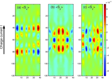
Figure 2: (Color online)Typical pattern of current-induced non-equilibrium spin density(in units of $\frac{h}{4\pi}$) in a two terminal structure. The lattice size for the central SO bar is $40\times 40$. The Rashba coupling strength is taken as $t_{R}$=0.1t.

To show clearly the characteristics of the current-induced spin polarization in a two-terminal structure, below we will study the spin density in the Rashba bar and in the leads separately. Firstly we study the spin density in the Rashba bar. The typical spin density pattern obtained in a two terminal structure is shown in Fig.2. From the figures one can see that the spatial distribution of the spin density inside the Rashba bar exhibits some apparent symmetry properties, which are summarized in Eq.(5) given below. Theoretically speaking, these symmetry properties are the results of some symmetry operations implicit in the two-terminal problem. Let us explain this point in some more detail. From the symmetry property of the Hamiltonian (1) and the rectangular geometry of the system shown in Fig.1, one can see that in our problem we have two symmetry operations $i\sigma_{y}P_{x}$ and $i\sigma_{x}P_{y}$, where $P_{x}$ and $P_{y}$ denote the spacial reflection manipulation $y\rightarrow-y$ and $x\rightarrow-x$ respectively and $i\sigma_{x}$ and $i\sigma_{y}$ the spin rotation manipulation with the angle $\pi$ around the $S_{x}$ and $S_{y}$ axes in spin space respectively. By considering these symmetry operations, from Eq.(4) one can obtain immediately the following symmetry relationsJiang2 :

$$<S_{x,z}(x,y)>_{I} = -<S_{x,z}(x,-y)>_{I}$$

$$<S_{y}(x,y)>_{I} = <S_{y}(x,-y)>_{I}$$

$$<S_{x}(x,y)>_{I} = -<S_{x}(-x,y)>_{I}$$

$$<S_{y,z}(x,y)>_{I} = <S_{y,z}(-x,y)>_{I},$$ (5)

where $<\cdots>_{I}$ stands for the spin density induced by a longitudinal charge current $I$ flowing from lead 1 to lead 2. The first two lines of Eq.(5) result from the symmetry operation $i\sigma_{y}P_{x}$, which has been known widely beforeSQShen2004 ; Zyang2005 . The second two, however, are results from the symmetry operation $i\sigma_{x}P_{y}$ and the $T$-reversal operation togetherJiang2 . Firstly, due to the $T$-reversal invariance, the equilibrium spin density vanishes when all chemical potentials are equal in Eq.(4), i.e., $<S_{\alpha}(x,y)>_{eq}=<S_{\alpha}(x,y)>_{I}+<S_{\alpha}(x,y)>_{-I}=0$, where $<S_{\alpha}(x,y)>_{-I}$ denotes the spin density induced by a longitudinal charge current $I$ from lead 2 to lead 1. Secondly, due to the geometry symmetry of the system under the manipulation $i\sigma_{x}P_{y}$, we have $<S_{x}(x,y)>_{I}=<S_{x}(x,y)>_{-I}$ and $<S_{y,z}(x,y)>_{I}=-<S_{y,z}(x,y)>_{-I}$. Combining these two results, we get the last two lines in Eq.(5).

In Fig.3 we plot the longitudinally averaged spin density inside the Rashba bar as a function of the transverse position $y$, where $<\vec{S}(y)>^{L}$denotes the longitudinal averaged value of $<\vec{S}(x,y)>$ along the $x$ direction ( i.e., the direction of the charge current flow ). Due to the symmetry relations shown in Eq.(5), the non-vanishing components are $<S_{y,z}(y)>^{L}$. Moreover, under the spatial reflection manipulation $y\rightarrow-y$, $<S_{y}(y)>^{L}$ is even and $<S_{z}(y)>^{L}$ is odd.

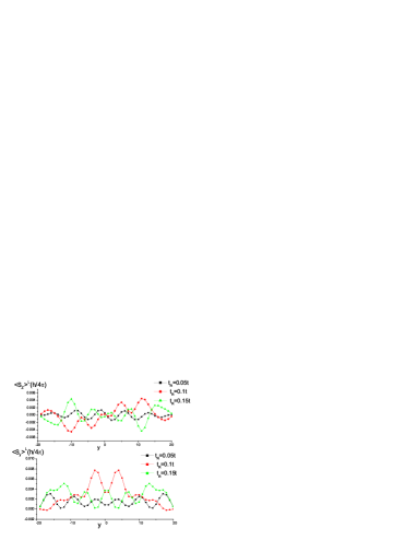
Figure 3: (Color online)Non-equilibrium spin density averaged in longitudinal direction in SO system , $<S_{y,z}>^{L}$, as a function of transverse position, y. The y and z components has different reflection symmetry with respect to x axis. The sign near the boundaries can be flipped by tuning Rashba coupling strength $t_{R}$.

The fact that the out-of-plane component $<S_{z}(y)>^{L}$ has opposite signs near the two lateral edges is consistent with the phenomenology of SHENikolic2005 ; WunderlichPRL2005 . But for a two-terminal lattice structure with general lattice sizes, our results show that the spin density does not always develop peak structures near the two boundaries but oscillate across the transverse direction. This is somehow different from the naive picture of spin accumulation near the boundaries due to a spin Hall current. The in-plane spin polarization is not related to the phenomenology of spin Hall effect. It can be regarded as a general magnetoelectric effect due to spin-orbit couplingHuangHu . It should be noted that, from the theoretical points of view, the relationship between spin current the induced spin polarization is actually a much subtle issue and is currently still under intensive debates. In this paper, however, we will free our discussions from such controversial issues.

It is evident from Fig. 3 that not only the magnitude, but also the sign of the spin accumulation near the two transverse boundaries can be changed by tuning the Rashba coupling strength. This is also reported in RefZyang2005 for a continuum two-terminal model. Since the Rashba coupling strength can be tuned experimentally through gate voltage, such a flipping behavior for spin accumulation might provide an interesting technological possibility for the electric control of the spin degree of freedom.

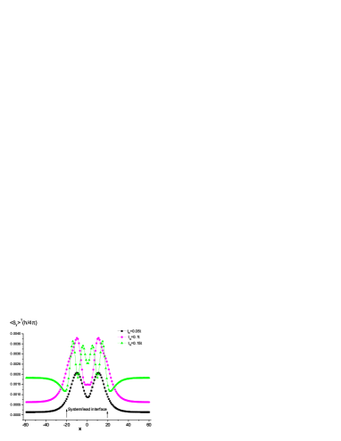
Figure 4: (Color online)The variation of spin density averaged in transverse direction of lead 2 versus Rashba coupling constant.

Now we present the most important theoretical prediction of this paper, i.e., the charge-current induced spin polarization effect in the contacted leads. Due to the first two lines in Eq.(5), after taking average in the transversal direction ( which will be denoted by $<S_{\alpha}>^{T}$ as a function of the longitudinal coordinate $x_{2}$ ), only $<S_{y}>^{T}$ will remain nonzero. In Fig. 4 $<S_{y}>^{T}$ is plotted versus the longitudinal coordinate $x$ of the whole system. The lattice size of the whole system is set to $120\times 40$, while the central $40\times 40$ lattice sites represents the Rashba SO bar (see Fig.1). As indicated clearly in the figure, the border between the Rashba bar and the contacted leads are at $x=\pm 20$. The Rashba SO coupling strength is chosen to be $t_{R}/t=0.05,0.1,0.15$. As can be seen from Fig. 4, $<S_{y}>^{T}$ changes with the coordinate $x$ both inside the Rashba bar and in the leads, but in the leads it changes with the coordinate $x$ only in a much narrow region close to the border between the leads and the Rashba bar and will reach to a fixed value further away from the border. This phenomenon is the lead spin polarization effect in this paper. Theoretically, this phenomenon can be understood as following. For an incident wave $(m,\sigma)$ with a Fermi energy $E_{f}$ in lead 1, the scattering wave function in lead 2 is: $\psi_{\sigma^{\prime}}^{1m\sigma}(x_{2},y_{2})=\sum_{n}\phi_{2n\sigma^{\prime}}^{1m\sigma}e^{ik_{n}x_{2}}\chi_{n}(y_{2})$, where $-2t\cos(k_{n})+\varepsilon_{n}=E_{f}$. Then the spin density $<\vec{S}(x_{2},y_{2})>$ can be calculated as ( dropping off a normalization factor ),

$$\sum_{m,\sigma}\frac{1}{v_{1m}}\sum_{\alpha,\beta}\psi_{\alpha}^{1m\sigma\ast}(x_{2},y_{2})\vec{\sigma}_{\alpha,\beta}\psi_{\beta}^{1m\sigma}(x_{2},y_{2}),$$

Thus, after taking average along the transversal direction, we have

$$<\vec{S}(x_{2})>^{T}=(1/N_{2})\sum_{y_{2}}<\vec{S}(x_{2},y_{2})>$$ (6)

$$\propto \sum_{m,\sigma}\frac{1}{v_{1m}}\sum_{n,\alpha,\beta}[\phi_{2n\alpha}^{1m\sigma}e^{-ik_{n}x_{2}})^{\ast}\vec{\sigma}_{\alpha,\beta}(\phi_{2n\beta}^{1m\sigma}e^{-ik_{n}x_{2}})],$$

where we have used the orthogonality relation for the transverse modes: $\sum_{y_{2}}\chi_{n}(y_{2})\chi_{n^{\prime}}(y_{2})=\delta_{nn^{\prime}}$. Evidently, the summand $[\cdots]$ in Eq. (6) is independent of $x_{2}$ as long as $k_{n}$ is real ( i.e., for those longitudinal propagating modes ). If $k_{n}$ is imaginary, the corresponding mode will describe an exponentially localized state in lead 2 in the vicinity of the border between the lead and the Rashba bar. Such evanescent componentsUsaj2005 can contribute to the local charge density and spin density only in the vicinity of the border. At some distance far away from the interface, the contribution of the evanescent modes to $<\vec{S}(x_{2})>^{T}$will decay exponentially as $x_{2}$ increase and hence $<\vec{S}(x_{2})>^{T}$ will be independent of $x_{2}$, as illustrated in Fig. 4.  This result implies that the spin polarization inside the Rashba bar can be inducted out by the driving charge current to the leads and manifest itself in an amplified way, i.e., the leads will become spin polarized and thus an electric-controllable spin state in the leads can be realized. Such a lead spin polarization effect might be more easily detectable by magnetic or optical methods than the spin polarization inside the mesoscopic Rashba bar.

The results presented above is obtained in the absence of impurity scattering. To simulate spin-independent disorder scattering, we assume a uniformly distributed random potential $w\in[-W_{D},W_{D}]$ in the Rashba bar with a disorder strength $W_{D}$. The non-equilibrium spin density can be obtained by taking average for a number of random realizations of local potentials. We averaged 1000 random realizations in all calculations. In Fig. 5 we show how the curves of $<S_{y}>^{T}$ versus $\ x$ change with $W_{D}$. All curves are calculated with $t_{R}=0.1t$. Noticeably, inside the Rashba bar the height of $<S_{y}>^{T}$decreases with increasing $W_{D}$ but the lead spin polarization will firstly increase in the weak disorder regime ( $W_{D}<0.5t$ ) and then decrease in the stronger disorder regime ( note that our calculations are carried out under the condition of a fixed longitudinal charge current density). Thus, there exists a certain regime in which disorder can enhance the saturation value of the spin polarization in the leads. The slight asymmetric form of $W_{D}=2t$ line means that we need to take more random configurations of local potential for large $W_{D}$ value, which is reasonable. Of course, there are some other factors such as spin-orbit coupling or impurity scattering in the leads that may reduce or suppress the lead spin polarization effect. Further quantitative study is needed in order to clarify the role of these factors.

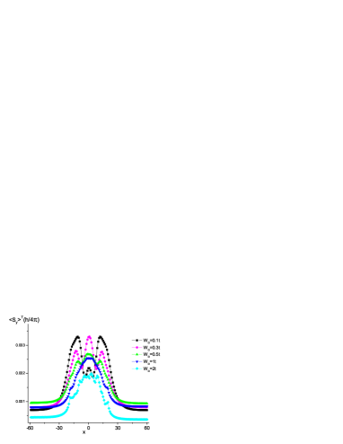
Figure 5: (Color online)The variation of spin density averaged in transverse direction versus longitudinal coordinate at the presence of disorder scattering.

IV Conclusion

To conclude, in this paper we have presented a theoretical study on the non-equilibrium lead spin polarization effect in a two-terminal mesoscopic Rashba bar under the condition of a fixed longitudinal charge current density. We have predicted that a finite amount of non-equilibrium spin polarizations can be induced in the leads by the spin-orbit coupling inside the mesoscopic Rashba bar when the longitudinal charge current circulate through it. Such a lead spin polarization effect can survive in the presence of weak disorder inside the Rashba bar and thus might be observable in real experiment. Such an effect might provide a new kind of electric-controllable spin state which is technically attractive. But it should be stressed that, for real systems, due to the existence of disorder scattering or spin-orbit interactions or other spin decoherence effects in the leads, the lead spin polarization effect predicted in the present paper may be weakened. These factors need to be clarified by more detailed theoretical investigations in the future.