Numerical Investigation of Light Scattering
off Split-Ring Resonators

Abstract

It seems to be feasible in the near future to exploit the properties of left-handed metamaterials in the telecom or even in the optical regime. Recently, split ring-resonators (SRR’s) have been realized experimentally in the near infrared (NIR) and optical regime [1, 2]. In this contribution we numerically investigate light propagation through an array of metallic SRR’s in the NIR and optical regime and compare our results to experimental results.

We find numerical solutions to the time-harmonic Maxwell’s equations by using advanced finite-element-methods (FEM). The geometry of the problem is discretized with unstructured tetrahedral meshes. Higher order, vectorial elements (edge elements) are used as ansatz functions. Transparent boundary conditions (a modified PML method [3]) and periodic boundary conditions [4] are implemented, which allow to treat light scattering problems off periodic structures.

This simulation tool enables us to obtain transmission and reflection spectra of plane waves which are incident onto the SRR array under arbitrary angles of incidence, with arbitrary polarization, and with arbitrary wavelength-dependencies of the permittivity tensor. We compare the computed spectra to experimental results and investigate resonances of the system.

Copyright 2005 Society of Photo-Optical Instrumentation Engineers.
This paper was published in Proc. SPIE 5955, p. 18 - 26 (2005), (Metamaterials ; Tomasz Szoplik, Ekmel Özbay, Costas M. Soukoulis, Nikolay I. Zheludev; Eds.). and is made available as an electronic reprint with permission of SPIE. One print or electronic copy may be made for personal use only. Systematic or multiple reproduction, distribution to multiple locations via electronic or other means, duplication of any material in this paper for a fee or for commercial purposes, or modification of the content of the paper are prohibited.

1 Introduction

With the advances in nanostructure physics it has become possible to manipulate light on a lengthscale smaller than optical wavelengths [1, 2]. It is now possible to construct periodic structures made of artifical nanostructures with macroscopic properties which do not occur in nature. These nanostructures are large on the atomic scale, therefore they can be of complex geometry. But they are small on the scale of the wavelength of the illuminating light, therefore the system has properties of an effective homogeneous material, in particular a macroscopical electric permittivity, $\varepsilon$, and magnetic permeability, $\mu$.

Of special interest are metamaterials with both, negative $\varepsilon$ and negative $\mu$ [5]. This leads to a negative index of refraction [6, 7] and allows in principle to overcome limits in the resolution of optical imaging systems [8].

2 Arrays of Split-Ring Resonators

Split-ring resonators can be understood as small $LC$ circuits consisting of an inductance $L$ and a capacitance $C$. The circuit can be driven by applying external electromagnetic fields. Near the resonance frequency of the $LC-$oscillator the induced current can lead to a magnetic field opposing the external magnetic field. When the SRR’s are small enough and closely packed – such that the system can be described as an effective medium – the induced opposing magnetic field corresponds to an effective negative permeability, $\mu<0$, of the medium.

Arrays of SRR’s with resonances in the NIR and in the optical regime have been fabricated using electron-beam lithography on a 1 mm thick glass substrate coated with a 5 nm thick film of indium-tin-oxide (ITO). Figure 1 shows electron micrographs of a produced sample. The ’U’-shaped SRR’s are produced with a thickness of $\Delta z=30\,$nm. Details on the production can be found in previous works [1, 2].

\psfrag{(a)}{(a)}\psfrag{(b)}{(b)}\includegraphics[width=433.62pt]{epse/micrograph_1}

Figure 1: Electron micrographs of an array of SRR’s with different magnifications. Field of view corresponds to approximately $8.5\,\mu$m$\times 7.6\,\mu$m (a), resp. $1.25\,\mu$m$\times 1.0\,\mu$m (b). The total size of the fabricated array is $100\,\mu$m$\times 100\,\mu$m. (See original publication for images with higher resolution.)

Due to the small dimensions of the $LC$ circuits their resonances are in the NIR and optical regime [2]. The elementary vectors of the periodic array, $\vec{a}_{1}=(315\,\mbox{nm},\,0,\,0)$ and $\vec{a}_{2}=(0,\,330\,\mbox{nm},\,0)$, are smaller than NIR and optical wavelengths, therefore in these regimes the system is well described as an effective medium.

In what follows we investigate numerically the transmission of light under oblique incidence through these samples.

\psfrag{}{}\psfrag{(a)}{}\psfrag{ax}{$a_{x}$}\psfrag{ay}{$a_{y}$}\psfrag{lx}{$l_{x}$}\psfrag{ly}{$l_{y}$}\psfrag{t}{$\Delta z$}\psfrag{d}{d}\psfrag{w}{w}\psfrag{x}{x}\psfrag{y}{y}\psfrag{z}{z}\psfrag{gold}{gold}\psfrag{ITO}{ITO}\includegraphics[width=195.12767pt]{epse/srr_geometry}

Figure 2: Geometry of the unit cell in the array of SRRs. The surrounding air and the substrate are not indicated. (See original publication for images with higher resolution.)

3 Light Propagation in Periodic Arrays of SRRs

We consider light scattering off a system which is periodic in the $x-$ and $y-$directions and is enclosed by homogeneous substrate (at $z_{sub}$) and superstrate (at $z_{sup}$) which are infinite in the $-$, resp. $+z-$direction. Light propagation in this system is governed by Maxwell’s equations where we assume vanishing densities of free charges and currents. The dielectric coefficient $\varepsilon(\vec{x})$ and the permeability $\mu(\vec{x})$ are periodic and complex, $\varepsilon\left(\vec{x}\right)=\varepsilon\left(\vec{x}+\vec{a}\right)$, $\mu\left(\vec{x}\right)=\mu\left(\vec{x}+\vec{a}\right)$. Here $\vec{a}$ is any elementary vector of the periodic lattice [9]. For given primitive lattice vectors $\vec{a}_{1}$ and $\vec{a}_{2}$ the elementary cell $\Omega\subset\mathbb{R}^{3}$ is defined as $\Omega=\left\{\vec{x}\in\mathbb{R}^{2}\,|\,x=\alpha_{1}\vec{a}_{1}+\alpha_{2}\vec{a}_{2};0\leq\alpha_{1},\alpha_{2}<1\right\}\times[z_{sub},z_{sup}].$ A time-harmonic ansatz with frequency $\omega$ and magnetic field ${\boldsymbol{H}}(\vec{x},t)=e^{-i\omega t}{\boldsymbol{H}}(\vec{x})$ leads to the following equations for ${\boldsymbol{H}}(\vec{x})$:

• The wave equation for the magnetic field:

  $$\nabla\times\frac{1}{\varepsilon(\vec{x})}\,\nabla\times{\boldsymbol{H}}(\vec{x})-\omega^{2}\mu(\vec{x}){\boldsymbol{H}}(\vec{x})=0,\qquad\vec{x}\in\Omega,$$ (1)

• The divergence condition for the magnetic field:

  $$\nabla\cdot\mu(\vec{x}){\boldsymbol{H}}(\vec{x})=0,\qquad\vec{x}\in\Omega,$$ (2)

• Transparent boundary conditions at the boundaries to the substrate (at $z_{sub}$) and superstrate (at $z_{sup}$), $\partial\Omega$, where ${\boldsymbol{H}}^{in}$ is the incident magnetic field (plane wave in this case), and $\vec{n}$ is the normal vector on $\partial\Omega$:

  $$\left(\frac{1}{\varepsilon(\vec{x})}\nabla\times({\boldsymbol{H}}-{\boldsymbol{H}}^{in})\right)\times\vec{n}=DtN({\boldsymbol{H}}-{\boldsymbol{H}}^{in}),\qquad\vec{x}\in\partial\Omega.$$ (3)

  The $DtN$ operator (Dirichlet-to-Neumann) is in our case realized with the PML method (perfectly matched layer) [3]. It is a generalized formulation of Sommerfeld’s radiation condition and can be realized alternatively, e.g., by the Pole condition method [10, 11].

• Furthermore, the Bloch theorem applies for wave propagation in periodic media. Therefore we aim to find Bloch-type field distributions [9] solving Equation (1), defined as

  $${\boldsymbol{H}}(\vec{x})=e^{i{\vec{k}}\cdot\vec{x}}{\boldsymbol{u}}(\vec{x}),\qquad{\boldsymbol{u}}(\vec{x})={\boldsymbol{u}}(\vec{x}+\vec{a}),$$ (4)

  where $\vec{a}$ is any elementary vector of the periodic lattice and the Bloch wavevector ${\vec{k}}\in\mathbb{R}^{3}$ is defined by the incoming plane wave ${\boldsymbol{H}}^{in}$.

Similar equations are found for the electric field ${\boldsymbol{E}}(\vec{x},t)=e^{-i\omega t}{\boldsymbol{E}}(\vec{x})$.

For applying the method of finite elements to solve Equations (1) – (4), resp. the corresponding equations for the electric field, it is necessary to reformulate these in the weak form. Care has to be taken in the right choice of functional spaces which are then discretized by Nedelec’s edge elements. This leads to a large sparse matrix equation (algebraic problem). For details on the weak formulation, the choice of Bloch-periodic functional spaces, the FEM discretization, and our implementation of the PML method we refer to previous works [3, 4, 12].

$a_{x}$ [nm]	315.0
$a_{y}$ [nm]	330.0
$l_{x}$ [nm]	200.0
$l_{y}$ [nm]	200.0
$w$ [nm]	90.0
$d$ [nm]	70.0
$\Delta z$ [nm]	30.0
$\Delta z_{ITO}$ [nm]	5.0
$\epsilon_{Substrate}$	2.25
$\epsilon_{ITO}$	3.8
$\epsilon_{air}$	1.0
$\epsilon_{gold}$	Drude model ($\omega_{p},\omega_{c}$)
$\omega_{p}$ [s-1]	$1.367\cdot 10^{16}$
$\omega_{c}$ [s-1]	$6.478\cdot 10^{13}$

Table 1: Geometrical parameters and material parameters for the SRR simulations corresponding to the experimental measurements reported by Enkrich et al [2]. (See original publication for images with higher resolution.)

To solve the algebraic problem on a standard personal computer we use either standard linear algebra decomposition techniques (LU-factorization) or iterative methods, depending on the problem size. Multi-grid algorithms [13] are used within the algorithm for preconditioning. As finite-element ansatz functions, we typically choose edge elements of second order [14]. Due to the use of multi-grid algorithms, the computational time and the memory requirements grow linearly with the number of unknowns.

4 Spatial discretization and material parameters

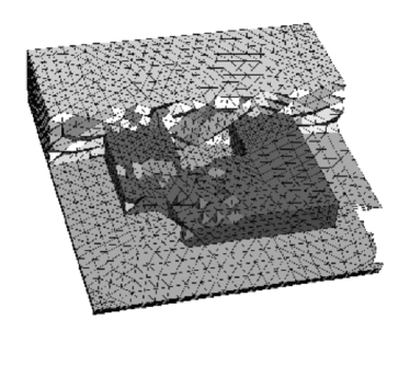
Figure 3: Visualization of a part of the tetrahedra of the spatial discretization of the SRR geometry shown in Figure 2. Dark gray tetrahedra: gold SRR; light gray: air; gray: ITO. Prism elements discretizing the exterior domain are not shown.(See original publication for images with higher resolution.)

Figure 2 shows the geometry of the unit cell of the array of investigated split-ring resonators. The geometrical parameters (corresponding to the experimentally realized SRR, see Fig. 1) are listed in Table 1. This unit cell corresponds to the computational domain $\Omega$ (see Equation 1) of the FEM simulations.

We discretize the computational domain using a 3D mesh generator [15]. This leads to a coarse unstructured tetrahedral mesh containing around $10^{3}$ tetrahedra. During the execution of the simulation this mesh is refined to a finer mesh (several refinement steps, in each of which every tetrahedron is refined to eight smaller tetrahedra). Figure 3 shows elements of a refined mesh. Obviously, by using such unstructured meshes, irregular geometries with nearly arbitrary shapes of the scatterers can be resolved ideally. In order to realize transparent boundary conditions with the PML method we discretize the exterior space with prism elements above and below the sample. The coarse grid in this case contains 1680 prisms which support second-order finite elements.

In the investigated regime, we assume a dependency of the permittivity of gold on the light frequency given by the Drude model:

$$\epsilon(\omega)=1-\frac{\omega_{p}^{2}}{\omega(\omega+i\omega_{c})}\quad,$$ (5)

with the plasma frequency $\omega_{p}$ and the collisional frequency $\omega_{c}$. The used parameters as well as the assumed permittivities of the other present materials are given in Table 1.

5 Numerical results

The discrete problem corresponding to Equations (1) – (4) with the parameters of Chapter 4 leads to a matrix equation with $N=28\,600$ unknowns for the coarse grid, resp. $N=133\,326$ unknowns for the one time uniformly refined grid. This equation is solved by LU factorization (package ’PARDISO’ [16]) on a standard 64bit PC (AMD Opteron). Typical computation times are 30 sec ($N=28\,600$), resp. 5 min ($N=133\,326$).

\psfrag{(a)}{(a)}\psfrag{(b)}{(b)}\includegraphics[width=325.215pt]{epse/solution_0deg}

Figure 4: Cross sections through the projection onto the $x-y-$plane of the 3D vectorial solutions at the center of the SRR ($15\,$nm above the ITO layer). (a) Electric field, (b) magnetic field. Parameters: $\lambda=1560\,$nm, incident wave polarized in the $x-z-$plane (${\boldsymbol{E}}$), resp. in the $y-z-$plane (${\boldsymbol{H}}$), perpendicular incidence. Please note that the magnetic field in the inner of the SRR points mainly in the $z-$direction, which is not seen in this presentation of the data.(See original publication for images with higher resolution.)

Cross-section of the 3D vectorial solutions, ${\boldsymbol{E}}(\vec{x})$ and ${\boldsymbol{H}}(\vec{x})$, for $z=const.$ at the center of the SRR is shown in Figure 4. In this case the wavelength of the incident plane wave is $\lambda=1.56\,\mu$m, and the incidence is perpendicular ($\vec{k}=|2\pi/\lambda|\times(0,\,0,\,-1)$). The polarization of the electric field of the incident wave is in the $x-z-$plane, i.e., $E_{0}=(1.0,\,0,\,0)\,$V/m.

In order to obtain the transmission coefficient for light scattered into the zero${}^{t}h$ diffraction order we perform a Fourier transform of the solution at the bottom of the computational domain ($z=z_{sub}$):

$$A_{i}(\vec{k}_{FC})=\frac{1}{a_{x}\cdot a_{y}}\int_{-a_{x}/2}^{a_{x}/2}\int_{-a_{y}/2}^{a_{y}/2}E_{i}(x,y,z_{sub})\exp(-i\vec{k}_{FC}\vec{x})dx\,dy$$ (6)

where $\vec{k}_{FC}$ is the projection of the wavevector of the zero${}^{t}h$ diffraction order onto the $x-y-$plane ($\vec{k}_{FC}=0$ for perpendicular incidence). In accordance with the convention used in the experiments [1, 2] we then define the transmission as $T=\frac{I_{t}}{\alpha I_{in}}$, where $\alpha$ corresponds to the transmission of a plane wave through a sample without SRR’s, $I_{in}$ is the intensity of the incoming wave, and $I_{t}$ is the intensity of the transmitted zero-order plane wave corresponding to the Fourier coefficients $A_{i}$. The reflection, $R$, is defined accordingly.

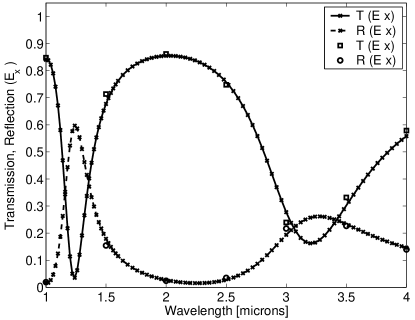
Figure 5: Transmission and reflection of a lightfield incident onto an SRR. Parameters correspond to the experiment of Linden et al. [1], Figure 2A. Please note the very good quantitative agreement with the experimental results. Transmission and reflection have been simulated on a coarse grid (x’s and solid, resp. dashed, lines) and on a refined grid (squares/circles).(See original publication for images with higher resolution.)

Figure 5 shows the calculated transmission and reflection of a light field with perpendicular incidence on a SRR. The comparison of the results obtained from simulations on the coarse grid (with $N=76\,014$ in this case) with the results obtained on a refined grid ($N=374\,366$) for several wavelengths (squares and circles in Figure 5) shows that for the investigated regime simulations with around $10^{5}$ unknowns are already well converged and the error in $T$ and $R$ can be estimated to be less than few percent.

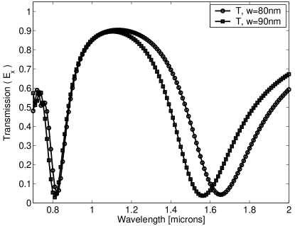
Figure 6: Transmission spectra of light fields incident onto an SRR. All SRR parameters correspond to Table 1 except for $w$ which is $w=80\,$nm (circles), resp. $w=90\,$nm (squares). (See original publication for images with higher resolution.)

The physics of the resonances of the SRR excited by the incident light field (around $\lambda=1.25\,\mu$m and $\lambda=3.2\,\mu$m in Figure 5) has been explained in detail in previous works [1, 2]. As an example of the strong dependence of the resonances on the geometrical parameters of the SRR’s we present in Figure 6 two transmission spectra for light fields (perpendicular incidence, ${\boldsymbol{E}}-$field in the $x-z-$plane) incident on SRR’s with parameters according to Table 1, except for the width of the lower bar of the ’U’ which is varied by a width of 10 nm.

\psfrag{(a)}{(a)}\psfrag{(b)}{(b)}\includegraphics[width=433.62pt]{epse/spectra_alpha}

Figure 7: Transmission spectra of light fields incident onto an SRR for different angles of incidence. Polarization of the incident ${\boldsymbol{E}}-$field in $x-$direction (a), resp. $y-$direction (b). (See original publication for images with higher resolution.)

\psfrag{x}{$x$}\psfrag{y}{$y$}\psfrag{(a)}{$\omega t=0$}\psfrag{(b)}{$\omega t=0.25\,\pi$}\psfrag{(c)}{$\omega t=0.5\,\pi$}\psfrag{(d)}{$\omega t=0.75\,\pi$}\psfrag{(e)}{$\omega t=1.0\,\pi$}\psfrag{(f)}{$\omega t=1.25\,\pi$}\psfrag{(g)}{$\omega t=1.5\,\pi$}\psfrag{(h)}{$\omega t=1.75\,\pi$}\includegraphics[width=325.215pt]{epse/phases_780nm_60deg}

Figure 8: Cross sections of the solution in $x-y-$direction in the region of the SRR and at the center of the SRR ($15\,$nm above the ITO layer). Shown is the projection of the real part of the ${\boldsymbol{E}}-$field onto the $x-y-$plane for different phases $\omega t$ of the time-harmonic solution. The exciting light field has a wavelength of $\lambda=780\,$nm and is incident with an angle of $\alpha=60\,$deg (solution corresponds to the low-wavelength resonance in Fig. 7b). (See original publication for images with higher resolution.)

By applying light fields which are incident onto the arrays of SRR under oblique angle, it is possible to observe several effects: Resonances can be excited now by the magnetic field component of the incident light field, resonances are shifted, and new, asymmetric resonances can be observed. Figure 7 shows simulated spectra for different angles of incidence. In Fig. 7a, the $\vec{k}$ vector of the incident plane wave is in the $y-z-$plane and encloses angles of $\alpha=0,30,45,60\,$deg with the $z-$axis, in Fig. 7b, the $\vec{k}$ vector of the incident plane wave is in the $x-z-$plane and again encloses angles of $\alpha=0,30,45,60\,$deg with the $z-$axis. The electric field is polarized in $x-$direction (a), resp. $y-$direction (b) (compare Figure 2 in ref [2]). All simulations are performed using a refined grid with $N=133\,326$ unknowns. It is again noted that in the case of oblique incidence special care has to be taken about the appropriate periodic boundary conditions in $x-$ and $y-$direction (see Equation 4). In very good quantitative agreement with the experimental results [2] the main effect of an increased angle $\alpha$ in case (a) seems to be an increase in linewidth of the resonance around 1.55 $\mu$m. This can intuitively explained by the fact that in this case the resonance is excited by a coupling of the electric field to the lower bar of the ‘U’-shaped SRR, which is not affected by a change of angle $\alpha$. However, the broadening can probably be attributed to the fact that the cross-section of the lower bar has a substantially larger horizontal dimension than vertical dimension.

The resonance around 1.55 $\mu$m can not be excited by the electric field in case (b). But, as the angle $\alpha$ is increased the $z-$component of the magnetic field of the incident wave is increased, too. This component couples to the resonance of the SRR. Therefore, around $\lambda=1.55\,\mu$m in case (b), and for $\alpha=60\,$deg a weak resonance of the SRR can be observed. Again, position as well as strength of the resonance are in quantitative very good agreement with the experimental results [2].

Interestingly, in case (b) the resonance around $\lambda=850\,$nm is shifted to higher wavelengths for increased angle $\alpha$, which can be attributed to the phase shift between the induced currents in the two upper arms of the ’U’-shaped SRR. Moreover, another resonance around $\lambda=780\,nm$ appears which is not excited in the case of perpendicular incidence of the plane wave. Figure 8 shows cross-sections through the real part of the electric field present in the SRR at different phases of the time-harmonic solution. From these distributions it can be seen that the resonance consists in oscillations of the electric field in both upper arms of the ’U’, with different amplitudes and phases, and an oscillation in the lower bar of the ’U’, which leads to an accumulation of charge at the outer bottom edges.

6 Conclusion

In this paper we have investigated rigorous numerical solutions of the 3D electromagnetic scattering problem of plane waves incident onto a periodic array of split-ring resonators in the optical regime. The solutions, obtained on standard personal computers, show an excellent agreement with experimental observations.

Future research directions include the investigation of systems with a macroscopically negative refractive index and nonlinear properties of metamaterials.

- [1] S. Linden, C. Enkrich, M. Wegener, C. Zhou, T. Koschny, and C. Soukoulis, “Magnetic response of metamaterials at 100 Terahertz,” Science 306, p. 1351, 2004.
- [2] C. Enkrich, M. Wegener, S. Linden, S. Burger, L. Zschiedrich, F. Schmidt, C. Zhou, T. Koschny, and C. M. Soukoulis, “Magnetic metamaterials at telecommunication and visible frequencies.” Phys. Rev. Lett., in press, preprint available from http://arxiv.org/pdf/cond-mat/0504774, 2005.
- [3] L. Zschiedrich, R. Klose, A. Schädle, and F. Schmidt, “A new finite element realization of the perfectly matched layer method for Helmholtz scattering problems on polygonal domains in 2D,” J. Comp. Phys., in press , 2005.
- [4] S. Burger, R. Klose, A. Schädle, F. Schmidt, and L. Zschiedrich, “FEM modelling of 3d photonic crystals and photonic crystal waveguides,” in Integrated Optics: Devices, Materials, and Technologies IX, Y. Sidorin and C. A. Wächter, eds., 5728, pp. 164–173, Proc. SPIE, 2005.
- [5] V. G. Veselago, “The electrodynamics of substances with simultaneously negative values of and ,” Sov. Phys. Usp. 10, p. 509, 1968.
- [6] D. R. Smith, W. J. Padilla, D. C. Vier, S. C. Nemat-Nasser, and S. Schultz, “Composite medium with simultaneously negative permeability and permittivity,” Phys. Rev. Lett. 84, p. 4184, 2000.
- [7] R. A. Shelby, D. R. Smith, and S. Schultz, “Experimental verification of a negative index of refraction,” Science 292, p. 77, 2001.
- [8] J. B. Pendry, “Negative refraction makes a perfect lens,” Phys. Rev. Lett. 85, p. 3966, 2000.
- [9] K. Sakoda, Optical Properties of Photonic Crystals, Springer-Verlag, Berlin, 2001.
- [10] T. Hohage, F. Schmidt, and L. Zschiedrich, “Solving Time-Harmonic Scattering Problems Based on the Pole Condition I: Theory,” SIAM J. Math. Anal. 35(1), pp. 183–210, 2003.
- [11] T. Hohage, F. Schmidt, and L. Zschiedrich, “Solving Time-Harmonic Scattering Problems Based on the Pole Condition II: Convergence of the PML Method,” SIAM J. Math. Anal. 35(3), pp. 547–560, 2003.
- [12] L. Zschiedrich, S. Burger, R. Klose, A. Schädle, and F. Schmidt, “JCMmode: An adaptive finite element solver for the computation of leaky modes,” in Integrated Optics: Devices, Materials, and Technologies IX, Y. Sidorin and C. A. Wächter, eds., 5728, pp. 192–202, Proc. SPIE, 2005.
- [13] P. Deuflhard, F. Schmidt, T. Friese, and L. Zschiedrich, Adaptive Multigrid Methods for the Vectorial Maxwell Eigenvalue Problem for Optical Waveguide Design, pp. 279–293. Mathematics - Key Technology for the Future, Springer-Verlag, Berlin, 2003.
- [14] P. Monk, Finite Element Methods for Maxwell’s Equations, Claredon Press, Oxford, 2003.
- [15] J. Schöberl, “Netgen.” Available from http://www.hpfem.jku.at.
- [16] O. Schenk et al., “Parallel sparse direct linear solver PARDISO.” Department of Computer Science, Universität Basel.