Exact numerical methods for electron-phonon problems

1 Introduction

In the last few years solid state physics has increasingly benefited from scientific computing and the significance of numerical techniques is likely to keep on growing quickly in this field. Because of the high complexity of solids, which are made of a huge number of interacting electrons and nuclei, a full understanding of their properties cannot be developed using analytical methods only. Numerical simulations do not only provide quantitative results for the properties of specific materials but are also widely used to test the validity of theories and analytical approaches.

Numerical and analytical approaches based on perturbation theory and effective independent-particle theories such as the Fermi liquid theory, the density functional theory, the Hartree-Fock approximation, or the Born-Oppenheimer approximation, have been extremely successful in explaining the properties of solids. However, the low-energy and low-temperature electronic, optical, or magnetic properties of various novel materials are not understood within these simplified theories. For example, in strongly correlated systems, the interactions between constituents of the solid are so strong that they can no longer be considered separately and a collective behavior can emerge. As a result, these systems may exhibit new and fascinating macroscopic properties such as high-temperature superconductivity or colossal magneto-resistance [2]. Quasi-one-dimensional electron-phonon (EP) systems like MX-chain compounds are other examples of electronic systems that are very different from traditional ones [3]. Their study is particularly rewarding for a number of reasons. First they exhibit a remarkably wide range of competing forces, which gives rise to a rich variety of different phases characterized by symmetry-broken ground states and long-range orders. Second these systems share fundamental features with higher-dimensional novel materials (for instance, high-$T_{\rm c}$ cuprates or charge-ordered nickelates) such as the interplay of charge, spin, and lattice degrees of freedom. One-dimensional (1D) models allow us to investigate this complex interplay, which is important but poorly understood also in 2D- and 3D highly correlated electron systems, in a context more favorable to numerical simulations.

1.1 Models

Calculating the low-energy low-temperature properties of solids from first principles is possible only with various approximations which often are not reliable in strongly correlated or low-dimensional electronic systems. An alternative approach for investigating these materials is the study of simplified lattice models which include only the relevant degrees of freedom and interactions but nevertheless are believed to reproduce the essential physical properties of the full system.

A fundamental model for 1D correlated electronic systems is the Hubbard model [4] defined by the Hamiltonian

$$H_{\rm ee}=-t\sum_{\langle i,j\rangle;\sigma}\left(c_{i\sigma}^{{\dagger}}c^{\phantom{{\dagger}}}_{j\sigma}+c_{j\sigma}^{{\dagger}}c^{\phantom{{\dagger}}}_{i\sigma}\right)+U\sum_{i}n_{i\uparrow}n_{i\downarrow}.$$ (1)

It describes electrons with spin $\sigma=\uparrow,\downarrow$ which can hop between neighboring sites on a lattice. Here $c^{{\dagger}}_{i\sigma}$, $c^{\phantom{{\dagger}}}_{i\sigma}$ are creation and annihilation operators for electrons with spin $\sigma$ at site $i$, $n_{i\sigma}=c^{{\dagger}}_{i\sigma}c^{\phantom{{\dagger}}}_{i\sigma}$ are the corresponding density operators. The hopping integral $t$ gives rise to a a single-electron band of width $4tD$ (with $D$ being the spatial dimension). The Coulomb repulsion between electrons is mimicked by a local Hubbard interaction $U\geq 0$. The average electronic density per site is $0<n<2$, where $n=N_{\rm e}/N$, $N$ is the number of lattice sites and $N_{\rm e}$ is the number of electrons; $n/2$ is called the band filling.

In the past the Hubbard model was intensively studied with respect to (itinerant) ferromagnetism, antiferromagnetism and metal-insulator (Mott) transitions in transition metals. More recently it has been used in the context of heavy fermions and high-temperature superconductivity as perhaps the most fundamental model accounting for strong electronic correlation effects in solids.

The coupling between electrons and the lattice relaxation and vibrations (phonons) is also known to have significant effects on the properties of solids including the above mentioned strongly correlated electronic materials (see the papers by Egami, Calvani, Zhou, Perroni, and Saini). Dynamical phonon effects are particularly important in quasi-1D metals and charge-density-wave (CDW) systems. The simplest model describing the effect of an additional EP coupling is the Holstein-Hubbard model. This model describes electrons coupled to dispersionless phonons, represented by local Einstein oscillators. The Hamiltonian is given by

$$H_{\rm ep}=H_{\rm ee}+\frac{1}{2M}\sum_{i}p^{2}_{i}+\frac{K}{2}\sum_{i}q^{2}_{i}-\alpha\sum_{i}q_{i}n_{i},$$ (2)

where $q_{i}$ and $p_{i}$ are the position and momentum operators for a phonon mode at site $i$, and $n_{i}=n_{i\uparrow}+n_{i\downarrow}$. At first sight, there are three additional parameters in this model (compared to the purely electronic model): The oscillator mass $M$, the spring constant $K$, and the EP coupling constant $\alpha$. However, if we introduce phonon (boson) creation and annihilation operators $b^{\dagger}_{i}$ and $b^{\phantom{{\dagger}}}_{i}$, respectively, the Holstein-Hubbard Hamiltonian can be written (up to a constant term)

$$H_{\rm ep}=H_{\rm ee}+\omega_{0}\sum_{i}b^{\dagger}_{i}b^{\phantom{{\dagger}}}_{i}-g\omega_{0}\sum_{i}(b^{\dagger}_{i}+b^{\phantom{{\dagger}}}_{i})n_{i}^{\phantom{{\dagger}}},$$ (3)

where the phonon frequency is given by $\omega_{0}^{2}=K/M$ ($\hbar=1$) and a dimensionless EP coupling constant is defined by $g=\alpha a/\omega_{0}$ with the range of zero-point fluctuations given by $2a^{2}=(KM)^{-1/2}$. We can set the parameter $a$ equal to 1 by redefining the units of oscillator displacements. Thus, the effects of the EP coupling are determined by two dimensionless parameter ratios only: $\omega_{0}/t$ and $g$. Alternatively, one can use the polaron binding energy $\varepsilon_{\rm p}=g^{2}\omega_{0}$ or, equivalently, $\lambda=\varepsilon_{\rm p}/2tD$, instead of $g$. The various constituents and couplings of the Holstein-Hubbard model are summarized in fig. 1.

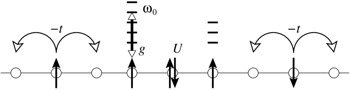
Figure 1: Schematic representation of the 1D Holstein-Hubbard model.

In the single-electron case, the resulting Holstein model [5] has been studied as a paradigmatic model for polaron formation (see the paper by Fehske, Alvermann, Hohenadler and Wellein). At half-filling, the EP coupling may lead to a Peierls instability related to the appearance of CDW order in competition with the SDW instability triggered by $U$ (see the separate paper by Fehske and Jeckelmann).

1.2 Methods

Despite the great simplification brought by the above models, theoretical investigations remain difficult because a quantum many-particle problem has to be solved with high accuracy to determine correlation effects on physical properties beyond the mean-field level. Analytical solutions of these models are known for special cases only. To determine the spectral and thermodynamical properties of these models, theorists have turned to numerical simulations. Among the various approaches, exact numerical methods play a significant role. A numerical calculation is said to be exact if no approximation is involved aside from the restriction imposed by finite computational resources (in particular, the same calculation would be mathematically exact if it were carried out analytically), the accuracy can be systematically improved with increasing computational effort, and actual numerical errors are quantifiable or completely negligible. Especially for strongly correlated systems, exact numerical methods are often the only approach available to obtain accurate quantitative results in model systems and the results that they provide are essential for checking the validity of theories or testing the accuracy of approximative analytical methods. Nowadays, finite-cluster exact diagonalizations (ED), the numerical renormalization group (NRG), density matrix renormalization group (DMRG) calculations, quantum Monte Carlo (QMC) simulations, and the dynamical mean-field theory (DMFT) have become very powerful and important tools for solving many-body problems. In what follows, we briefly summarize the advantages and weaknesses of these techniques, especially in the context of EP lattice models such as the the Holstein-Hubbard model. Then in the remaining sections we will present the basic principles of the ED (sect. 2) and DMRG (sect. 3 and 4) approaches.

The paradigm of an exact numerical calculation in a quantum system is the exact diagonalization (ED) of its Hamiltonian, which can be carried out using several well-established algorithms (see the next section). ED techniques can be used to calculate most properties of any quantum system. Unfortunately, they are restricted to small systems (for instance, 16 sites for a half-filled Hubbard model and less for the Holstein-Hubbard model) because of the exponential increase of the computational effort with the number of particles. In many cases, these system sizes are too small to simulate adequately macroscopic properties of solids (such as (band) transport, magnetism or charge long-range order). They are of great value, however, for a description of local or short-range order effects.

In QMC simulations the problem of computing quantum properties is transformed into the summation of a huge number of classical variables, which is carried out using statistical (Monte Carlo) techniques. There are numerous variations of this principle also for EP problems (see, e.g., the paper on QMC by Mishchenko). QMC simulations are almost as widely applicable as ED techniques but can be applied to much larger systems. The results of QMC calculations are affected by statistical errors which, in principle, can be systematically reduced with increasing computational effort. Therefore, QMC techniques are often numerically exact. In practice, several problems such as the sign problem (typically, in frustrated quantum systems) or the large auto-correlation time in the Markov chain (for instance, in critical systems) severely limit the applicability and accuracy of QMC simulations in strongly correlated or low-dimensional systems. Moreover, real-frequency dynamical properties often have to be calculated from the imaginary-time correlation functions obtained with QMC using an analytic continuation. However, the transformation of imaginary-time data affected by statistical errors to real-frequency data is an ill-conditioned numerical problem. In practice, one has to rely on approximate transformations using least-square or maximum-entropy fits, which yield results of unknown accuracy.

DMRG methods allow us to calculate the static and dynamical properties of quantum systems much larger than those possible with ED techniques (see the third and fourth section, as well as the separate paper by Fehske and Jeckelmann). For 1D systems and quantum impurity problems, one can simulate lattice sizes large enough to determine static properties in the thermodynamic limit and the dynamical spectra of macroscopic systems exactly. In higher dimensions DMRG results are numerically exact only for system sizes barely larger than those available with ED techniques. For larger system sizes in dimension two and higher DMRG usually provides only a variational approximation of the system properties.

The NRG is a precursor of the DMRG method. Therefore, it it not surprising that most NRG calculations can also be carried out with DMRG. NRG provides numerically exact results for the low-energy properties of quantum impurity problems (see the paper on NRG methods by Hewson). Moreover, for this type of problem it is computationally more efficient than DMRG. For other problems (lattice problems, high-energy properties) NRG usually fails or provides results of poor accuracy.

In the dynamical mean-field theory (see the papers by Ciuchi, Capone, and Castellani) it is assumed that the self-energy of the quantum many-body system is momentum-independent. While this is exact on a lattice with an infinitely large coordination number (i.e., in the limit of infinite dimension), it is considered to be a reasonable approximation for 3D systems. Thus in applications to real materials DMFT is never an exact numerical approach, although a DMFT-based approach for a 3D system could possibly yield better results than direct QMC or DMRG calculations. It should be noticed that in the DMFT framework the self-energy has to be determined self-consistently by solving a quantum impurity problem, which is itself a difficult strongly correlated problem. This quantum impurity problem is usually solved numerically using one of the standard methods discussed here (ED, NRG, QMC or DMRG). Therefore, the DMFT approach and its extensions can be viewed as an (approximate) way of circumventing the limitations of the standard methods and extend their applicability to large 3D systems.

In summary, every numerical method has advantages and weaknesses. ED is unbiased but is restricted to small clusters. For 1D systems DMRG is usually the best method while for 3D systems only direct QMC simulations are possible. QMC techniques represent also the most successful approach for non-critical and non-frustrated two-dimensional systems. There is currently no satisfactory numerical (or analytical) method for two-dimensional strongly correlated systems with frustration or in a critical regime.

2 Exact diagonalization approach

As stated above, ED is presently probably the best controlled numerical method because it allows an approximation-free treatment of coupled electron-phonon models in the whole parameter range. As a precondition we have to work with finite systems and apply a well-defined truncation procedure for the phonon sector (see subsect. 2.1). At least for the single-electron Holstein model a variational basis can be constructed in such a way that the ground-state properties of the model can be computed numerically exact in the thermodynamic limit (cf. subsect. 2.2). In both cases the resulting numerical problem is to find the eigenstates of a (sparse) Hermitian matrix using Lanczos or other iterative subspace methods (subsect. 2.3). In general the computational requirements of these eigenvalue algorithms are determined by matrix-vector multiplications (MVM), which have to be implemented in a parallel, fast and memory saving way on modern supercomputers. Extensions for the calculation of dynamical quantities have been developed on the basis of Lanczos recursion and kernel polynomial expansions (cf. subsect. 2.4). Quite recently cluster perturbation theory (CPT) has been used in combination with these techniques to determine the single-particle electron and phonon spectra.

2.1 Many-body Hilbert space and basis construction

2.1.1 Basis symmetrization

The total Hilbert space of Holstein-Hubbard type models (2) can be written as the tensorial product space of electrons and phonons, spanned by the complete basis set $\left\{|b\rangle=|e\rangle\otimes|p\rangle\right\}$ with

$$|e\rangle=\prod_{i=1}^{N}\prod_{\sigma=\uparrow,\downarrow}(c_{i\sigma}^{\dagger})^{n_{i\sigma,e}}|0\rangle_{e}\quad\mbox{and}\quad|p\rangle=\prod_{i=1}^{N}\frac{1}{\sqrt{m_{i,p}!}}(b_{i}^{\dagger})^{m_{i,p}}|0\rangle_{p}.$$ (4)

Here $n_{i\sigma,e}\in\{0,1\}$, i.e. the electronic Wannier site $i$ might be empty, singly or doubly occupied, whereas we have no such restriction for the phonon number, $m_{i,p}\;\in\{0,\ldots,\infty\}.$ Consequently, $e=1,\ldots,D_{e}$ and $p=1,\ldots,D_{p}$ label basic states of the electronic and phononic subspaces having dimensions $D_{e}=\genfrac{(}{)}{0.0pt}{1}{N}{N_{e,\sigma}}\genfrac{(}{)}{0.0pt}{1}{N}{N_{e,-\sigma}}$ and $D_{p}=\infty$, respectively. Since the Holstein Hubbard Hamiltonian commutes with the total electron number operator $\hat{N}_{e}=\sum_{i=1}^{N}(n_{i,\uparrow}+n_{i,\downarrow})$, $\hat{N}_{e,\sigma}=\sum_{i=1}^{N}n_{i,\sigma}$ (we used the ‘hat’ to discriminate operators from the corresponding particle numbers), and the $z$-component of the total spin $S^{z}=\frac{1}{2}\sum_{i=1}^{N}(n_{i,\uparrow}-n_{i,\downarrow})$, the basis $\left\{|b\rangle\right\}$ has been constructed for fixed $N_{e}$ and $S^{z}$.

To further reduce the dimension of the total Hilbert space, we can exploit the space group symmetries [translations ($G_{T}$) and point group operations ($G_{L}$)] and the spin-flip invariance [($G_{S}$); $S^{z}=0$ – subspace only]. Clearly, working on finite bipartite clusters in 1D or 2D (here $N=k^{2}+l^{2}$, $k$ and $l$ are both even or odd integers) with periodic boundary conditions (PBC), we do not have all the symmetry properties of the underlying 1D or 2D (square) lattices [6]. Restricting ourselves to the 1D non-equivalent irreducible representations of the group $G(\vec{K})=G_{T}\times G_{L}(\vec{K})\times G_{S}$, we can use the projection operator ${\cal P}_{\vec{K},rs}=[g(\vec{K})]^{-1}\sum_{{\cal G}\in G(\vec{K})}\chi_{\vec{K},rs}^{(\cal G)}\;{\cal G}$ (with $[H,{\cal P}_{\vec{K},rs}]=0$, ${\cal P}_{\vec{K},rs}^{\dagger}={\cal P}_{\vec{K},rs}$ and ${\cal P}_{\vec{K},rs}\;{\cal P}_{\vec{K}^{\prime},r^{\prime}s^{\prime}}={\cal P}_{\vec{K},rs}\;\delta_{\vec{K},\vec{K}^{\prime}}\;\delta_{r,r^{\prime}}\;\delta_{s,s^{\prime}}$) in order to generate a new symmetrized basis set: $\{|b\rangle\}\stackrel{{\scriptstyle\cal P}}{{\to}}\{|\tilde{b}\rangle\}$. ${\cal G}$ denotes the $g(\vec{K})$ elements of the group $G(\vec{K})$ and $\chi_{\vec{K},rs}^{(\cal G)}$ is the (complex) character of ${\cal G}$ in the $[\vec{K},rs]$ representation, where $\vec{K}$ refers to one of the $N$ allowed wave vectors in the first Brillouin zone, $r$ labels the irreducible representations of the little group of $\vec{K}$, $G_{L}(\vec{K})$, and $s$ parameterizes $G_{S}$. For an efficient parallel implementation of the MVM it is extremely important that the symmetrized basis can be constructed preserving the tensor product structure of the Hilbert space, i.e.,

$$\{|\tilde{b}\rangle=N^{[\vec{K}rs]}_{\tilde{b}}\,{\cal P}_{\vec{K},rs}\,\left[|\tilde{e}\rangle\otimes|p\rangle\right]\},$$ (5)

with $\tilde{e}=1,\ldots,\tilde{D}_{e}^{g(\vec{K})}$ $[\tilde{D}_{e}^{g(\vec{K})}\sim D_{e}/g(\vec{K})]$. The $N^{[\vec{K}rs]}_{\tilde{b}}$ are normalization factors.

2.1.2 Phonon Hilbert space truncation

Since the Hilbert space associated to the phonons is infinite even for a finite system, we apply a truncation procedure [7] retaining only basis states with at most $M$ phonons:

$$\{|p\rangle\;;\;m_{p}=\sum^{N}_{i=1}m_{i,p}\leq M\}.$$ (6)

The resulting Hilbert space has a total dimension $\tilde{D}=\tilde{D}_{e}^{g(\vec{K})}\times D_{p}^{M}$ with $D_{p}^{M}=\frac{(M+N)!}{M!N!}$, and a general state of the Holstein Hubbard model is represented as

$$|\psi_{\vec{K},rs}\rangle=\sum_{\tilde{e}=1}^{\tilde{D}_{e}^{g(\vec{K})}}\sum_{p=1}^{D^{M}_{p}}c_{\tilde{e}p}\,|\tilde{b}\rangle.$$ (7)

It is worthwhile to point out that, switching from a real-space representation to a momentum space description, our truncation scheme takes into account all dynamical phonon modes. This has to be contrasted with the frequently used single-mode approach [8]. In other words, depending on the model parameters and the band filling, the system “decides” by itself how the $M$ phonons will be distributed among the independent Einstein oscillators related to the $N$ Wannier sites or, alternatively, among the $N$ different phonon modes in momentum space. Hence with the same accuracy phonon dynamical effects on lattice distortions being quasi-localized in real space (such as polarons, Frenkel excitons, …) or in momentum space (like charge-density-waves, …) can be studied.

Of course, one has carefully to check for the convergence of the above truncation procedure by calculating the ground-state energy as a function of the cut-off parameter $M$. In the numerical work convergence is assumed to be achieved if $E_{0}$ is determined with a relative error $\Delta E_{0}^{(M)}=(E_{0}(M)-E_{0}(M-1))/E_{0}(M)\leq 10^{-6}$ . In addition we guarantee that the phonon distribution function

$$|c^{(m)}|^{2}(M)=\sum^{\tilde{D}^{g(\vec{K})}_{e}}_{\tilde{e}=1}\sum^{D^{M}_{p}}_{\stackrel{{\scriptstyle{\displaystyle{}_{p=1}}}}{{\{m_{p}=m\}}}}|c_{\tilde{e}p}|^{2},$$ (8)

which gives the different weights of the $m$-phonon states in the ground-state $|\psi_{0}\rangle$, becomes independent of $M$ and $|c^{(M)}|^{2}(M)\leq 10^{-6}$. To illustrate the $M$ dependences of the phonon distribution function and the ground-state energy, we have shown both quantities in fig. 2 for the single-electron Holstein model on rather small lattices. Figure 2 proves that our truncation procedure is well controlled even in the strong EP coupling regime, where multi-phonon states become increasingly important.

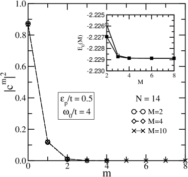
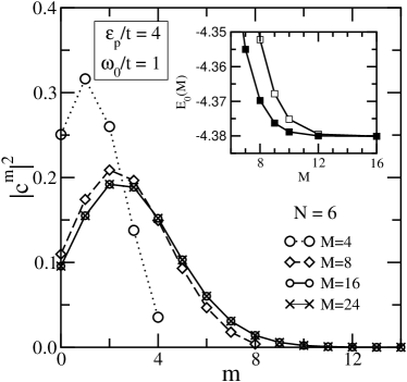
Figure 2: Convergence of the phonon distribution function $|c^{m}|^{2}(M)$ and ground-state energy $E_{0}(M)$ (inset; here filled symbols give the results obtained separating the $Q=0$ phonon mode) as a function of the maximum number of phonons $M$ retained. Results are given for the Holstein model on a 1D lattice with $N=14$ (a) and $N=6$ (b) sites (PBC), where the parameters $\varepsilon_{p}$ and $\omega_{0}$ are the same as for the CPT calculation presented in fig. 3 of the paper by Fehske, Alvermann, Hohenadler and Wellein.

For the Holstein-type models the computational requirements can be further reduced. Here it is possible to separate the symmetric phonon mode, $B_{0}=\frac{1}{\sqrt{N}}\sum_{i}b_{i}$, and to calculate its contribution to $H$ analytically [9]. For the sake of simplicity, we restrict ourselves to the 1D spinless case in what follows. Using the momentum space representation of the phonon operators, the original Holstein Hamiltonian takes the form

$$H=-t\sum_{ij}(c^{\dagger}_{i}c_{j}+c^{\dagger}_{j}c_{i})-\sqrt{\varepsilon_{p}\omega_{0}}\;\sum_{j}({B^{\dagger}_{-Q_{j}}}+{B_{Q_{j}}}){n}_{Q_{j}}+\omega_{0}\sum_{j}B^{\dagger}_{Q_{j}}B_{Q_{j}}$$ (9)

with $B_{Q_{j}}^{\dagger}={\cal U}_{j,i}b^{\dagger}_{i}$, $B_{Q_{j}}={\cal U}_{j,i}^{*}b_{i}={\cal U}_{-j,i}b_{i}$, and $n_{Q_{j}}=\sum_{i}{\cal U}_{j,i}n_{i}$, where ${\cal U}_{j,i}=(1/\sqrt{N})\times$
$\exp{\{iQ_{j}R_{i}\}}$ and $Q_{j}$ ($R_{i}$) denote the allowed momentum (translation) vectors of the lattice. The $Q=0$ phonon mode couples to $n_{0}=N_{e}/\sqrt{N}$ which is a constant if working in a subspace with fixed number of electrons. Thus the Hamiltonian decomposes into $H=H^{\prime}+H_{Q=0}$, with $H_{Q=0}=-\sqrt{\varepsilon_{p}\omega_{0}}\,({B^{\dagger}_{0}}+{B_{0}})\,n_{0}+\omega_{0}B^{\dagger}_{0}B_{0}$. Since $[H^{\prime},H_{Q=0}]=0$, the eigenspectrum of $H$ can be built up by the analytic solution for $H_{Q=0}$ and the numerical results for $H^{\prime}$. Using the unitary transformation

$${\cal\bar{S}}(N_{e})=\exp{\left\{-\frac{N_{e}}{\sqrt{N}}\sqrt{\frac{\varepsilon_{p}}{\omega_{0}}}({B^{\dagger}_{0}}-{B_{0}})\right\}}$$ (10)

which introduces a shift of the phonon operators ($B_{0}\rightarrow B_{0}+\frac{N_{e}}{\sqrt{N}}\sqrt{\frac{\varepsilon_{p}}{\omega_{0}}}$), we easily find the diagonal form of $\bar{H}_{Q=0}=\omega_{0}B^{\dagger}_{0}B_{0}-\varepsilon_{p}N^{2}_{e}/N$. It represents a harmonic oscillator with eigenvalues and eigenvectors $\bar{E}_{\bar{l}}=\omega_{0}\bar{l}-\varepsilon_{p}\frac{N^{2}_{el}}{N}$ and $|\bar{l}\rangle=\frac{1}{\sqrt{\bar{l}!}}(B^{\dagger}_{0})^{\bar{l}}|0\rangle$. The corresponding eigenenergies and eigenvectors of $H_{Q=0}$ are $E_{l}=\bar{E}_{\bar{l}}$ and $|l(N_{e})\rangle={\cal\bar{S}}^{\dagger}(N_{e})|\bar{l}\rangle$, respectively. That is, in the eigenstates of the Holstein model a homogeneous lattice distortion occurs. Note that the homogeneous lattice distortions are different in subspaces with different electron number. Thus excitations due to lattice relaxation processes will show up in the one-particle spectral function. Finally, eigenvectors and eigenenergies of $H$ can be constructed by combining the above analytical result with the numerically determined eigensystem ($E^{\prime}_{n}$; $|\psi_{n}^{\prime}\rangle$) of $H^{\prime}$: $E_{n,l}^{\prime}=E_{n}^{\prime}+\omega_{0}l-\varepsilon_{p}N^{2}_{e}/N$ and $|\psi_{n,l}\rangle=|\psi_{n}^{\prime}\rangle\otimes|l(N_{e})\rangle$.

2.2 Variational ED method

In this section we briefly outline a very efficient variational method to address the (one-electron) Holstein polaron problem numerically in any dimension. The approach was developed by Bonča et al. [10, 11] and is based on a clever way of constructing the EP Hilbert space which can be systematically expanded in order to achieve high-accuracy results with rather modest computational resources.

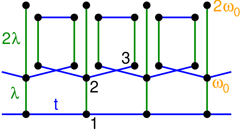
Figure 3: Small variational Hilbert space for the 1D polaron problem. Basis states are represented by dots, off-diagonal matrix elements by lines. Vertical bonds create or destroy phonons with frequency $\omega_{0}$. Horizontal bonds correspond to electron hops $(\propto t)$. Accordingly, state $|1\rangle$ describes an electron at the origin (0) and no phonon, state $|2\rangle$ is an electron and one phonon both at site 0, $|3\rangle$ is an electron at the nearest neighbor-site site 1, and a phonon at site 0, and so on. The figure is re-drawn from ref. [10].

The authors built up the variational space starting from an initial state, e.g. the electron at the origin, and acting repeatedly ($L$ times) with the off-diagonal diagonal hopping ($t$) and EP coupling ($\lambda$) terms of the Hamiltonian (see fig. 3). A basis state is added if it is connected by a non-zero $t$- or $\lambda$-matrix element to a state previously in the space, i.e., states in generation $l$ are obtained by acting $l$ times with off-diagonal terms. Only one copy of each state is retained. Importantly, all translations of these states on an infinite lattice are included. According to Bloch’s theorem each eigenstate can be written as $\psi=\mbox{e}^{{\rm i}kj}a_{L}$, where $a_{L}$ is a set of complex amplitudes related to the states in the unit cell, e.g. $L=7$ for the small variational space shown in fig. 3. For each momentum $K$ the resulting numerical problem is then to diagonalize a Hermitian $L\times L$ matrix. While the size of the Hilbert space increases as (D+1)^L, the error in the ground-state energy decreases exponentially with $L$. Thus in most cases $10^{4}$-$10^{6}$ basis states are sufficient to obtain an 8-10 digit accuracy for $E_{0}$. The ground-state energy calculated this way is variational for the infinite system.

2.3 Solving the eigenvalue problem

To determine the eigenvalues of large sparse Hermitian matrices, iterative (Krylov) subspace methods like Lanczos [12] and variants of Davidson [13] diagonalization techniques are frequently applied. These algorithms contain basically three steps:

• project problem matrix ${\bf A}$ $\in\mathbb{R}^{n}$ onto a subspace $\bar{\bf A}^{k}\in\mathbb{V}^{k}$ $(k\ll n)$

• solve the eigenvalue problem in $\mathbb{V}^{k}$ using standard routines

• extend subspace $\mathbb{V}^{k}\to\mathbb{V}^{k+1}$ by a vector $\vec{t}\perp\mathbb{V}^{k}$ and go back to (2).

This way we obtain a sequence of approximative inverses of the original matrix ${\bf A}$.

2.3.1 Lanczos diagonalization

Starting out from an arbitrary (random) initial state $|\varphi_{0}\rangle$, having finite overlap with the true ground state $|\psi_{0}\rangle$, the Lanczos algorithm recursively generates a set of orthogonal states (Lanczos or Krylov vectors):

$$|\varphi_{l+1}\rangle={\bf H}^{\tilde{D}}|\varphi_{l}\rangle-a_{l}|\varphi_{l}\rangle-b_{l}^{2}|\varphi_{l-1}\rangle,$$ (11)

where $a_{l}=\langle\varphi_{l}|{\bf H}^{\tilde{D}}|\varphi_{l}\rangle/\langle\varphi_{l}|\varphi_{l}\rangle,b_{l}^{2}=\langle\varphi_{l}|\varphi_{l}\rangle/\langle\varphi_{l-1}|\varphi_{l-1}\rangle,b_{0}^{2}=0$, and $|\varphi_{-1}\rangle=0$. Obviously, the representation matrix $[{\bf T}^{L}]_{l,l^{\prime}}=\langle\varphi_{l}|{\bf H}^{\tilde{D}}|\varphi_{l^{\prime}}\rangle$ of ${\bf H}^{\tilde{D}}$ is tridiagonal in the $L$-dimensional Hilbert space spanned by the $\{|\varphi_{l}\rangle\}_{l=0,\ldots,L-1}$ ($L\ll\tilde{D}$):

$${\bf T}^{L}=\left(\begin{array}[]{cccccc}a_{0}&b_{1}&0&0&0&\cdots\\ b_{1}&a_{1}&b_{2}&0&0&\cdots\\ 0&b_{2}&a_{2}&b_{3}&0&\cdots\\ 0&0&b_{3}&a_{3}&b_{4}&\cdots\\ \vdots&\vdots&\vdots&\vdots&\vdots&\ddots\end{array}\right).$$ (12)

Applying the Lanczos recursion (11), the eigenvalues $E_{n}$ and eigenvectors $|\psi_{n}\rangle$ of ${\bf H}^{\tilde{D}}$ are approximated by

$$E_{n}^{L}\quad\mbox{ and}\quad|\psi^{L}_{n}\rangle=\sum_{l=0}^{L-1}c_{n,l}^{L}|\varphi_{l}\rangle,$$ (13)

respectively, where the L coefficients $c_{n,l}^{L}$ are the components of the ($n-{\rm th}$) eigenvectors of ${\bf T}^{L}$ with eigenvalue $E_{n}^{L}$. The eigenvalue spectrum of ${\bf T}^{L}$ can be easily determined using standard routines from libraries such as EISPACK (see http://www.netlib.org). Increasing $L$ we check for the convergence of an eigenvalue of ${\bf T}^{L}$ in a specific energy range. So we can avoid spurious eigenvalues for fixed Lanczos dimension $L$ which disappear as one varies $L$ [12].

Note that the convergence of the Lanczos algorithm is excellent at the edges of the spectrum (the ground state for example is obtained with high precession using at most $\sim 100$ Lanczos iterations) but rapidly worsens inside the spectrum. So Lanczos is suitably used only to obtain the ground state and a few low lying excited states.

2.3.2 Implementation of matrix vector multiplication

The core operation of most ED algorithms is a MVM. It is quite obvious that our matrices are extremely sparse because the number of non-zero entries per row of our Hamilton matrix scales linearly with the number of electrons. Therefore a standard implementation of the MVM step uses a sparse storage format for the matrix, holding the non-zero elements only. Two data schemes are in wide use, the compressed row storage (CRS) and the jagged diagonal storage (JDS) format [14], where the latter is the method of choice for vector computers. The typical storage requirement per non-zero entry is 12-16 Byte for both methods, i.e. for a matrix dimension of $\tilde{D}=10^{9}$ about one TByte main memory is required to store only the matrix elements of the EP Hamiltonian. Both variants can be applied to any sparse matrix structure and the MVM step can be done in parallel by using a parallel library such as PETSc (see http://www-unix.mcs.anl.gov/petsc/petsc-as/).

To extend our EP studies to even larger matrix sizes we store no longer the non-zero matrix elements but generate them in each MVM step. Of course, at that point standard libraries are no longer useful and a parallel code tailored to each specific class of Hamiltonians must be developed. For the Holstein-Hubbard EP model we have established a massively parallel program using the Message Passing Interface (MPI) standard. The minimal total memory requirement of this implementation is three vectors with Hilbert space dimension.

The parallelization approach follows the inherent natural parallelism of the Hilbert space, which can be constructed as the tensorial product space of electrons and phonons $\{|\tilde{b}\rangle=|\tilde{e}\rangle\otimes|p\rangle\}$ (cf. subsubsect. 2.1.1). Assuming, that the electronic dimension ($\tilde{D}_{e}$) is a multiple of the number of processors used ($N_{\rm cpu}$) we can easily distribute the electronic basis states among these processors, i.e. processor $i(0\leq i\leq N_{\rm cpu}-1)$ is holding the basis states ($\tilde{e}_{i}=i\tilde{D}_{e}/N_{\rm cpu}+1,\ldots,(i+1)D_{e}/N_{\rm cpu}$). As a consequence of this choice only the electronic hopping term generates inter-processor communication in the MVM while all other (diagonal electronic) contributions can be computed locally on each processor.

Furthermore, the communication pattern remains constant within a single run for all MVM steps and the message sizes (at least $D_{p}$ words) are large enough to ignore the latency problems of modern interconnects. Using supercomputers with hundreds of processors and one TBytes of main memory, such as IBM p690 clusters or SGI Altix systems, we are able to run simulations up to a matrix dimension of $30\times 10^{9}$.

2.4 Algorithms for estimating spectral functions

The numerical calculation of spectral functions

$$A^{\cal O}(\omega) = -\lim_{\eta\to 0^{+}}\frac{1}{\pi}\mbox{Im}\left[\langle\psi_{0}|{\bf O}^{\dagger}\frac{1}{\omega-{\bf H}+E_{0}+i\eta}{\bf O}|\psi_{0}\rangle\right]$$ (14)

$$= \sum_{n=0}^{\tilde{D}-1}|\langle\psi_{n}|{\bf O}|\psi_{0}\rangle|^{2}\delta[\omega-(E_{n}-E_{0})],$$

where ${\bf O}$ is the matrix representation of a certain operator ${\cal O}$ (e.g., the creation operator $c_{k}^{\dagger}$ of an electron with wave number $k$ if one wants to calculate the single-particle spectral function; or the current operator $\hat{\jmath}=-\mbox{i}et\sum_{i}(c_{i}^{\dagger}c_{i+1}-c_{i+1}^{\dagger}c_{i})$ if one is interested in the optical conductivity), involves the resolvent of the Hamilton matrix ${\bf H}$. Once we have obtained the eigenvalues and eigenvectors of $H$ we can plug them into eq. (14) and obtain directly the corresponding dynamical correlation or Green functions. In practice this ‘naive’ approach is applicable for small Hilbert spaces only, where the complete diagonalization of the Hamilton matrix is feasible.

For the typical EP problems under investigation we deal with Hilbert spaces having total dimensions $\tilde{D}$ of $10^{6}$-$10^{11}$. Finding all eigenvectors and eigenstates of such huge Hamilton matrices is impossible, because the CPU time required for exact diagonalization of ${\bf H}$ scales as $\tilde{D}^{3}$ and memory as $\tilde{D}^{2}$. Fortunately, there exist very accurate and well-conditioned linear scaling algorithms for a direct approximate calculation of $A^{\cal O}(\omega)$.

2.4.1 Lanczos recursion method

Having determined the ground state $|\psi_{0}^{L}\rangle$ by the Lanczos technique, we can use again the recursion relation (11), but with the initial state $|\varphi_{0}\rangle={\bf O}|\psi^{L}_{0}\rangle/\sqrt{\langle\psi^{L}_{0}|{\bf O}^{\dagger}{\bf O}|\psi^{L}_{0}\rangle}$, to determine within the so-called Lanczos recursion method (LRM) or spectral decoding method (SDM) an approximative spectral function,

$$\bar{A}^{\cal O}(\omega)=\sum_{n=0}^{L-1}|c_{n,0}^{L}|^{2}\langle\psi_{0}|{\bf O}^{\dagger}{\bf O}|\psi_{0}\rangle\,\delta[\omega-(E_{n}^{L}-E_{0}^{L})],$$ (15)

or equivalently

$$\bar{A}^{\cal O}(\omega)=-\lim_{\eta\to 0^{+}}\frac{1}{\pi}\mbox{Im}{\,\,\frac{\langle\psi_{0}|{\bf O}^{\dagger}{\bf O}|\psi_{0}\rangle}{\omega+\mbox{i}\eta-a_{0}-\cfrac{b_{1}^{2}}{\omega+{\rm i}\eta-a_{1}-\cfrac{b_{2}^{2}}{z-a_{2}-\cdots}}}}\,,$$ (16)

which is built up by $L$ $\delta$-peaks.

Of course, the true spectral function $A^{\cal O}(\omega)$ has $\tilde{D}$ $\delta$-peaks. According to the Lanczos phenomenon, the approximated spectral weights and positions of the peaks converge to their true values with increasing $L$. Some of the main problems of the LRM/SDM are: (i) The convergence is not uniform in the whole energy range. (ii) There exist so-called spurious peaks, which appear and disappear as $L$ is increased, i.e., when the iteration proceeds. (iii) Without computationally expensive re-orthogonalization only a few hundred iterations are possible.

2.4.2 Kernel polynomial method

The idea behind a conceptionally different approach, the kernel polynomial method (KPM) (for a review see [15]), is to expand $A^{\cal O}(\omega)$ in a finite series of $L+1$ Chebyshev polynomials $T_{m}(x)=\cos[m\arccos(x)]$. Since the Chebyshev polynomials are defined on the real interval $[-1,1]$, we apply first a simple linear transformation to the Hamiltonian and all energy scales: ${\bf X}=({\bf H}-b)/a$, $x=(\omega-b)/a$, $a=(E_{\rm max}-E_{\rm min})/2(1-\epsilon)$, and $b=(E_{\rm max}+E_{\rm min})/2$ (the small constant $\epsilon$ is introduced in order to avoid convergence problems at the endpoints of the interval –a typical choice is $\epsilon\sim 0.01$ which has only 1% impact on the energy resolution [16]). Then the expansion reads

$$A^{\cal O}(x)=\frac{1}{\pi\sqrt{1-x^{2}}}\left(\mu_{0}^{\cal O}+2\sum_{m=1}^{L}\mu_{m}^{\cal O}T_{m}(x)\right),$$ (17)

with the coefficients (moments)

$$\mu_{m}^{\cal O}=\int_{-1}^{1}dx\,T_{m}(x)A^{\cal O}(x)=\langle\psi_{0}|{\bf O}^{\dagger}T_{m}({\bf X}){\bf O}|\psi_{0}\rangle.$$ (18)

Equation (17) converges to the correct function for $L\to\infty$. Again the moments

$$\mu_{2m}^{\cal O}=2\langle\phi_{m}|\phi_{m}\rangle-\mu_{0}^{\cal O}\quad\mbox{and}\quad\mu_{2m+1}^{\cal O}=2\langle\phi_{m+1}|\phi_{m}\rangle-\mu_{1}^{\cal O}$$ (19)

can be efficiently obtained by repeated parallelized MVM, where $|\phi_{m+1}\rangle=2{\bf X}|\phi_{m}\rangle-|\phi_{m-1}\rangle$ but now $|\phi_{1}\rangle={\bf X}|\phi_{0}\rangle$ and $|\phi_{0}\rangle={\bf O}|\psi_{0}\rangle$ with $|\psi_{0}\rangle$ determined by Lanczos ED.

As is well known from Fourier expansion, the series (17) with $L$ finite suffers from rapid oscillations (Gibbs phenomenon) leading to a poor approximation to $A^{\cal O}(\omega)$. To improve the approximation the moments $\mu_{n}$ are modified $\mu_{n}\to g_{n}\mu_{n}$, where the damping factors $g_{n}$ are chosen to give the ‘best’ approximation for a given $L$. This modification is equivalent to a convolution of the infinite series with a smooth approximation $K_{L}(x,y)$ to $\delta(x-y)$, a so-called approximation kernel. The appropriate choice of this kernel, that is of $g_{n}$, e.g. to guarantee positivity of $A^{\cal O}(\omega)$, lies at the heart of KPM. We mainly use the Jackson kernel which results in a uniform approximation whose resolution increases as $1/L$, but for the determination of the single-particle Green functions below we use a Lorentz kernel which mimics a finite imaginary part $\eta$ in eq. (14), see [15].

In view of the uniform convergence of the expansion, KPM is a method tailored to the calculation of spectral properties. Most important, spectral functions obtained via KPM are not subject to uncontrolled or biased approximations: The accuracy of its outcome depends only on the expansion depth $L$, and can be made as good as required by just increasing $L$. Of course one is restricted to finite systems of moderate size whose associated Hamilton matrix does not exceed available computational resources.

2.4.3 Cluster perturbation theory (CPT)

The spectrum of a finite system of $N$ sites which we obtain through KPM differs in many respects from that in the thermodynamic limit $N\to\infty$, especially it is obtained for a finite number of momenta $K=\pi\,m/N$ only. The most obvious feature is the resulting discreteness of energy levels which is a property already of the non-interacting system. While we cannot easily increase $N$ without going beyond computationally accessible Hilbert spaces, we can try to extrapolate from a finite to the infinite system.

For this purpose we first calculate the Green function $G^{c}_{ij}(\omega)$ for all sites $i,j=1,\dots,N$ of a $N$-size cluster with open boundary conditions, and then recover the infinite lattice by pasting identical copies of this cluster at their edges. The ‘glue’ is the hopping $V$ between these clusters, where $V_{kl}=t$ for $|k-l|=1$ and $k,l\equiv 0,1\bmod N$, which is dealt with in first order perturbation theory. Then the Green function $G_{ij}(\omega)$ of the infinite lattice is given through a Dyson equation

$$G_{ij}(\omega)=G^{c}_{ij}(\omega)+\sum_{kl}G^{c}_{ik}(\omega)V_{kl}G_{lj}(\omega),$$ (20)

where indices of $G^{c}(\omega)$ are counted modulo $N$. Obviously this order of perturbation in $V$ is exact for the non-interacting system. We thus get rid of the discreteness addressed above. The Dyson equation is solved by Fourier transformation over momenta $K=kN$ corresponding to translations by $N$ sites

$$G_{ij}(K,\omega)=\left[\frac{G^{c}(\omega)}{1-V(K)G^{c}(\omega)}\right]_{ij},$$ (21)

from which one finally obtains

$$G(k,\omega)=\frac{1}{N}\sum_{i,j=1}^{N}G^{c}_{ij}(Nk,\omega)\exp(-\mathrm{i}k(i-j)).$$ (22)

In this way, which is called CPT [17], we obtain a Green function $G(k,\omega)$ with continuous momenta $k$ from the Green function $G^{c}_{ij}(\omega)$ on a finite cluster. Two approximations are made, one by using first order perturbation theory in $V=t$, the second on assuming translational symmetry in $G_{ij}(\omega)$ which is only approximatively satisfied.

In principle, the CPT spectral function $G(k,\omega)$ does not contain any more information than the cluster Green function $G^{c}_{ij}(\omega)$ already does. But extrapolating to the infinite system it gives a first hint at the scenario in the thermodynamic limit. However, CPT does not describe effects which only occur on large length scales, like Anderson localization (see the paper by Fehske, Bronold and Alvermann) or the critical behavior at a phase transition. Providing direct access to spectral functions, still without relying on possibly erroneous approximations, CPT occupies a niche between variational approaches like (D)DMRG (see sect. 3 and 4) and methods directly working in the thermodynamic limit like the variational ED method [10].

3 Density matrix renormalization group approach

The Density Matrix Renormalization Group (DMRG) is one of the most powerful numerical techniques for studying many-body systems. It was developed by Steve White [18] in 1992 to overcome the problems arising in the application of the standard Numerical Renormalization Group (NRG) to quantum lattice many-body systems such as the Hubbard model (1). Since then the approach has been extended to a great variety of problems, from Classical Statistical Physics to Quantum Chemistry (including ab initio calculations of electronic structures in molecules) and, recently, to Nuclear Physics and the Physics of Elementary Particles and Fields. A review article on DMRG and its numerous applications has recently been published [19]. Additional information can also be found on the DMRG web page at http://www.dmrg.info. A detailed discussion of the basic DMRG algorithms and their implementation has been published in ref. [20]. Readers interested in a simple example should consider the application of DMRG to single-particle problems, which is also discussed there. The source code of a single-particle DMRG program (in the programming language C⁺⁺) is now part of the ALPS distribution [21].

DMRG techniques for strongly correlated systems have been substantially improved and extended since their conception and have proved to be both extremely accurate for low-dimensional problems and widely applicable. They enable numerically exact calculations (as good as exact diagonalizations) of low-energy properties on large lattices with up to a few thousand particles and sites (compared to less than a few tens for exact diagonalizations). The calculation of high-energy excitations and dynamical spectra for large systems has proved to be more difficult and will be discussed in sect. 4.

3.1 Renormalization group and density matrix

Consider a quantum lattice system with $N$ sites (in general, we are interested in the case $N\rightarrow\infty$ or at least $N\gg 1$). The Hilbert space of this system is the Fock space of all properly symmetrized many-particle wave functions. As seen in sect. 2, its dimension $D$ grows exponentially with the number of sites $N$. Obviously, a lot of these states are not necessary to investigate specific properties of a model such as the ground state. Thus, a number of methods have been developed to perform a projection onto a subspace of dimension $d\ll D$ and then an exact diagonalization of the Hamiltonian in this subspace.

Such an approach, called the Numerical Renormalization Group (NRG), was developed by Wilson 30 years ago to solve the Kondo impurity problem [22]. The key idea is the decomposition of the system into subsystems with increasing size (see the paper on the NRG method by Hewson). The subsystem size is increased by one site at each step as shown in fig. 4. Each subsystem is diagonalized successively and the information obtained is used to truncate the Hilbert space before proceeding to the next larger subsystem. Let $m$ and $n$ be the dimension of the (effective) Hilbert spaces associated with the subsystem made of the first $\ell$ sites and with the site $\ell+1$, respectively. A basis of dimension $d=mn$ for the next subsystem with $\ell+1$ sites is built as a tensor product of the subsystem and site bases. Assuming that $d$ is small enough, the effective Hamiltonian can be fully diagonalized in the tensor-product basis. The energy is used as a criterion to truncate the subsystem Hilbert space. The lowest $m$ eigenstates are kept to form a new basis while the high-energy eigenstates are discarded. The new subsystem with $\ell+1$ sites and an effective Hilbert space of dimension $m$ can be used to start the next iteration. In summary, this procedure provides a transformation $H_{\ell+1}=R[H_{\ell}]$ forming effective Hamiltonians of fixed dimension $m$ which describe the low-energy physics of increasingly larger systems. In this transformation the high-energy states are steadily traced out as the system grows as illustrated in fig. 4. Such a transformation $R$ is usually called a renormalization group (RG) transformation. A different implementation of the NRG idea is possible if the system is homogeneous like in the Hubbard model. A copy of the current subsystem can be substituted for the added site in the above procedure. Thus the subsystem size doubles at every iteration as illustrated in fig. 4.

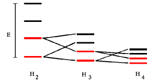
Figure 4: Schematic representations of the usual NRG algorithm (left), an alternative NRG algorithm (middle) and the energy levels in the effective Hamiltonian $H_{\ell}$ for increasing subsystem system size $\ell$ (right).

The NRG method is very accurate for the Kondo problem and more generally for quantum impurity problems. Unfortunately, NRG and related truncation schemes have proved to be unreliable for quantum lattice systems such as the Hubbard model [23]. It is easy to understand the failure of the standard NRG in those cases. A subsystem always has an artificial boundary at which the low-energy eigenstates of a quantum lattice Hamiltonian tend to vanish smoothly. Thus the truncation procedure based on the effective eigenenergies may keep only states that vanish at the artificial boundary. As a consequence, at later RG iterations the eigenstates of the effective Hamiltonian of larger subsystems may have unwanted features like nodes where the artificial boundary of the previous subsystems were located. The application of the second NRG algorithm (in the middle in fig. 4) to the problem of a quantum particle in a one-dimensional box gives a clear illustration of this effect [20, 24]. The ground state wavefunction for a $N$-site lattice $\phi(x)=\sqrt{\frac{2}{N+1}}\sin\left(\frac{\pi x}{N+1}\right)$ has a minimum (node) where the ground state wavefunction of the twice larger system ($N\rightarrow 2N$) has a maximum as seen in fig. 5. Therefore, the low-energy eigenstates of a small system are not necessarily the best states to form the low-energy eigenstates of a larger system. An approach proposed by White and Noack [24] to solve this problem is the construction of an effective Hamiltonian including the effects of the subsystem environment to eliminate the artificial boundary. DMRG is the extension of this idea to interacting many-particle problems.

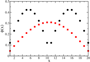
Figure 5: Ground-state wavefunctions of the tight-binding particle-in-the-box problem for two systems of $N=$10 sites (circles) and one system of $N=20$ sites (squares).

Consider a quantum system which can be split into two parts called the subsystem and its environment. A basis of the system Hilbert space is given by the tensor product

$$|i,j\rangle=|i\rangle\otimes|j\rangle_{\rm E}$$ (23)

of basis states $|i\rangle\ (i=1,\dots,d)$ and $|j\rangle_{\rm E}\ (j=1,\dots,d_{\rm E})$ for the subsystem and its environment, respectively. The dimension of this basis is $d_{\rm S}=d\cdot d_{\rm E}$. Any state $|\psi\rangle$ of the system can be expanded in this basis $|\psi\rangle=\sum_{i,j}\psi_{ij}\ |i\rangle\otimes|j\rangle_{\rm E}$ . The most important states in the subsystem to represent the state $|\psi\rangle$ are given by its reduced density matrix, which is obtained by tracing out the states of the environment

$$\rho_{i,i^{\prime}}=\sum_{j}\psi^{*}_{ij}\psi_{i^{\prime}j}.$$ (24)

This density matrix is symmetric and has $d$ positive eigenvalues $w_{\alpha}\geq 0$ satisfying the normalization $\sum_{\alpha}w_{\alpha}=1$. A new basis of the subsystem, $|v_{\alpha}\rangle=\sum_{i}v_{\alpha i}|i\rangle$, can be defined using the eigenvectors of the density matrix $\sum_{i^{\prime}}\rho_{i,i^{\prime}}v_{\alpha i^{\prime}}=w_{\alpha}v_{\alpha i};\alpha,i=1,\dots,d.$ In the new basis the state $|\psi\rangle$ can be written

$$|\psi\rangle=\sum_{\alpha}\lambda_{\alpha}|v_{\alpha}\rangle\otimes|u_{\alpha}\rangle_{\rm E},$$ (25)

with $\lambda^{2}_{\alpha}=w_{\alpha}>0$ and normalized states $|u_{\alpha}\rangle_{\rm E}=\frac{1}{\lambda_{\alpha}}\sum_{i,j}v^{*}_{\alpha i}\psi_{ij}|j\rangle_{\rm E}.$ Therefore, $w_{\alpha}$ is the probability that a subsystem is in a state $|v_{\alpha}\rangle$ if the superblock is in the state $|\psi\rangle$. The density matrix provides an optimal choice for selecting the $m$ states of the subsystem to be kept in a RG transformation: keep density matrix eigenstates $|v_{\alpha}\rangle$ with the largest weights $w_{\alpha}$. This is the key idea of the density matrix renormalization group approach.

3.2 DMRG algorithms

In a DMRG calculation one first forms a new subsystem with $\ell+1$ sites and an effective Hilbert space of dimension $d=mn$ by adding a site to the current subsystem with $\ell$ sites as in the NRG method. Then one considers a larger system, called a superblock, which is made of the new subsystem and an environment. A basis of the superblock Hilbert space is given by the tensor product (23). Assuming initially that we want to compute the system ground state only, we then calculate the ground state $|\psi\rangle$ of the superblock Hamiltonian using the techniques discussed in subsect. 2.3. Then the reduced density matrix (24) for the subsystem is obtained by tracing out the environment states. The $m$ density matrix eigenstates $|v_{\alpha}\rangle$ with the largest weights $w_{\alpha}$ are kept to build an optimal effective basis of dimension $m$ for the subsystem with $\ell+1$ sites. This subsystem is then used to start the next iteration and build the next larger subsystem. This procedure defines a generic density matrix RG transformation. Clearly, the accuracy of a DMRG calculation will depend on the quality of the environment used. The environment should make up as much as possible of the lattice which is not already included in the subsystem. Constructing such a large and accurate environment is as difficult as the original quantum many-body problem. Therefore, the environment must also be constructed self-consistently using a density matrix RG transformation.

In his initial papers [18], White described two DMRG algorithms: the infinite-system method and the finite-system method. The infinite-system method is certainly the simplest DMRG algorithm and is the starting point of many other algorithms. Its defining characteristic is that the environment is constructed using a “reflection” of the current subsystem. The superblock size increases by two sites at each step as illustrated in fig. 6. The system is assumed to be homogeneous and “symmetric” to allow this operation. Iterations are continued until an accurate approximation of an infinite system is obtained. The infinite-system method is sometimes used to calculate properties of finite systems. While this approach may work just fine in many cases, it should be kept in mind that there is no guarantee of convergence to the eigenstates of the finite system.

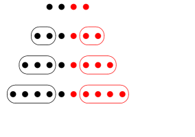
Figure 6: Schematic representation of DMRG algorithms. Left: Infinite-system algorithm (from top to bottom). Right: Finite-system DMRG algorithm for a ten-site lattice. The environment block is on the right-hand side when going from top to bottom and on the left-hand-side when going from bottom to top.

The finite-system method is the most versatile and reliable DMRG algorithm and with some later improvements [19, 20] it has also become a very efficient method. It is designed to calculate the properties of a finite system accurately. The environment is chosen so that the superblock represents the full lattice at every iteration. The environments can also be considered as being subsystems and are calculated self-consistently using DMRG with the usual subsystems playing the part of their environment. Iterations are continued back and forth through every configuration of the superblock (i.e., every splitting of the lattice in one subsystem and its environment) until convergence. This procedure is illustrated in fig. 6. This ensures the self-consistent optimization of the subsystems and their environments (for a given number $m$ of states kept) and thus considerably improves the results reliability compared to the infinite-system method.

Most DMRG algorithms use only two blocks (the subsystem and its environment) to form the superblock, but it is possible and useful for some problems to consider a more complicated configuration. For instance, one can use four blocks to treat one-dimensional problems with periodic boundary conditions and using several blocks can also be advantageous for systems with boson degrees of freedom such as phonons [25].

The DMRG sites usually correspond to the physical sites of the lattice model investigated, such as spin, fermionic, or bosonic degree of freedom. [For a phonon mode (boson), which has an infinite Hilbert space, a DMRG site represents a finite dimensional basis of the phonon states [26] as already discussed for exact diagonalization methods (subsect. 2.1).] However, the DMRG sites can also represent a combination of several physical sites [for instance, the electron and phonon at each site of the Holstein-Hubbard model (2)], a fraction of the Hilbert space associated with a given physical site (as in the pseudo-site method for bosonic degrees of freedom presented in subsubsect. 3.4.1).

It is possible to compute several quantum states simultaneously with DMRG. In that case, the density matrix is formed as the sum of the density matrices (24) calculated for each target state. A target state can be any quantum state which is well-defined (and can be computed) in every superblock of a DMRG calculation. This feature turns out to be very important for the calculations of dynamical properties (see sect. 4).

3.3 Truncation errors

With DMRG an error is made when projecting operators onto the subspace spanned by the most important $m$ density matrix eigenstates. This is called the truncation error. Probably the most important characteristic of a DMRG calculation is the rate at which the truncation error decreases with an increasing number $m$ of states kept. In the most favorable cases (gapped one-dimensional systems with short-range interactions only and open boundary conditions), the accuracy increases roughly exponentially with $m$. For instance, the ground-state energy of the spin-one Heisenberg chain on lattices with hundreds of sites can be calculated to an accuracy of the order of $10^{-10}$ with a modest computational effort. In very difficult cases (long-range off-diagonal interactions, two-dimensional systems with periodic boundary conditions), the truncation error in the ground state energy can decrease as slowly as $m^{-2}$. It is possible to calculate exactly the density matrix spectrum of several integrable models [27]. This analysis shows that the distribution of density matrix eigenvalues $w_{\alpha}$ varies greatly. As a result, truncation errors may fall exponentially with increasing $m$ in some favorable cases but decrease extremely slowly for other ones. Correspondingly, DMRG accuracy and performance depend substantially on the specific problem investigated.

For any target state $|\psi\rangle$ written down in its representation (25), the truncation of the density matrix basis corresponds to making an approximation

$$|\psi^{\prime}\rangle=\sum_{m\;\mbox{\scriptsize kept states}}\lambda_{\alpha}\ |v_{\alpha}\rangle\otimes|u_{\alpha}\rangle_{\rm E},$$ (26)

which minimizes the error

$$D_{m}=\left||\psi\rangle-|\psi^{\prime}\rangle\right|^{2}=\sum_{d-m\;\mbox{\scriptsize discarded states}}w_{\alpha}=1-\sum_{m\;\mbox{\scriptsize kept states}}w_{\alpha},$$ (27)

for a fixed number $m$ of states kept. The total weight of the discarded density matrix eigenstates (discarded weight) $D_{m}$ is related to the truncation errors of physical quantities. For $D_{m}\ll 1$ it can be shown that the truncation error in the eigenenergy of any target eigenstates of the Hamiltonian $H$ scales linearly with the discarded weight, $E^{\prime}_{m}-E_{\rm exact}=cD_{m}+\mathcal{O}(D_{m}^{2})\;,$ where $E^{\prime}_{m}=\langle\psi^{\prime}|H|\psi^{\prime}\rangle/\langle\psi^{\prime}|\psi^{\prime}\rangle$ is the energy in the approximate state $|\psi^{\prime}\rangle$ and $c$ is a constant. For the expectation values of other operators the truncation error theoretically scales as $\sqrt{D_{m}}$. The discarded weight $D_{m}$ decreases (and thus the accuracy of DMRG results increases) when the number $m$ of density matrix eigenstates kept is increased. In particular, for large enough $m$ the discarded weights vanish at every RG iteration for both subsystems and environments and truncation errors become negligible. Therefore, DMRG is an exact numerical method as defined in the introduction (sect. 1). Moreover, if the number $m$ of density matrix eigenstates kept is so large that the discarded weight is exactly zero at every RG iteration, DMRG becomes equivalent to an exact diagonalization (sect. 2).

In real DMRG applications, series of density matrix basis truncations are performed in successive superblock configurations. Therefore, the measured discarded weights $D_{m}$ do not represent the real error in the wave function of the target. Nevertheless, in most cases, the energy truncation error scales linearly with the average measured discarded weight $D_{m}$ for $D_{m}\ll 1$ as shown in fig. 7(a). This can (and should) be used to make an $D_{m}\rightarrow 0$ extrapolation of the energy. For other physical quantities such as an order parameter, truncation errors sometimes scale as $(D_{m})^{r}$, with $r\approx 0.5$ as seen in fig. 7(b). This can also be used to estimate truncation errors. The measured discarded weight $D_{m}$ alone should not be used as an indication of a calculation accuracy, because truncation errors for physical quantities can be several orders of magnitude larger than $D_{m}$.

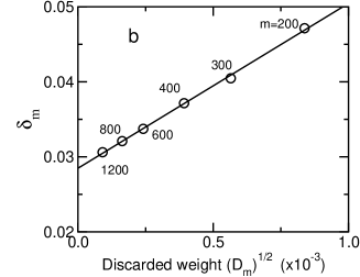
Figure 7: (a) Ground state energy $E^{\prime}_{m}$ calculated with DMRG for a $12\times 3$ Hubbard ladder with $U=t$ and 6 holes as a function of the discarded weight $D_{m}$ for several number of density matrix eigenstates kept $m=300$ to 2200. The zero of the energy is given by a (nearly) exact quantum Monte Carlo result [28]. (b) Staggered bond order parameter $\delta_{m}$ calculated with DMRG in an extended 1D half-filled Hubbard model [29] for $U=3t$ and $V=1.5t$ on a 1024-site lattice as a function of $\sqrt{D_{m}}$ for $m=200$ to 1200. Solid lines are linear fits.

It should be noted that DMRG can be considered as a variational approach. The system energy $E(\psi)=\langle\psi|H|\psi\rangle/\langle\psi|\psi\rangle$ is minimized in a variational subspace of the system Hilbert space to find the ground-state wavefunction $|\psi_{0}\rangle$ and energy $E_{0}=E(\psi_{0})$. If the ground-state wavefunction is calculated with an error of the order of $\epsilon\sim\sqrt{D_{m}}\ll 1$ (i.e., $|\psi\rangle=|\psi_{0}\rangle+\epsilon|\phi\rangle$, with $\langle\phi|\phi\rangle=1$), the energy obtained is an upper bound to the exact result and the error in the energy is of the order of $\epsilon^{2}\ (\sim D_{m}$) as in all variational approaches. For specific algorithms the variational wave function can be written down explicitly as a matrix product wave function or as a product of local tensors [19].

The computational effort of a DMRG calculation usually increases as a power law for increasing system size $N$, number $m$ of states kept, or DMRG site dimension $n$. In the most favorable case (1D system with short-range interactions only), the CPU time increases theoretically as $Nm^{3}n^{3}$, while the amount of stored data is of the order of $\sim m^{2}n^{2}$. In most cases, however, $m$ has to be increased with the system size $N$ to keep truncation errors constant.

3.4 Methods for electron-phonon systems

A significant limitation of DMRG and exact diagonalizations is that they require a finite basis for each site. In electron-phonon lattice models such as the Holstein-Hubbard model (2), the number of phonons (bosons) is not conserved and the Hilbert space is infinite for each site representing an oscillator. Of course, the number of phonons can be artificially constrained to a finite number $M$ per site, but the number $M$ needed for an accurate treatment may be quite large. This often severely constrains the system size or the regime of coupling which may be studied with DMRG [26] and exact diagonalizations (sect. 2).

Here, we describe two methods for treating systems including sites with a large Hilbert space. Both methods use the information contained in a density matrix to reduce the computational effort required for the study of such systems. The first method [30], called pseudo-site method, is just a modification of the usual DMRG technique which allows us to deal more efficiently with sites having a large Hilbert space. The second method [31, 32], called the optimal basis method, is a procedure for generating a controlled truncation of the phonon Hilbert space, which allows the use of a very small optimal basis without significant loss of accuracy.

3.4.1 Pseudo-site method

The DMRG algorithms presented above can easily be generalized to treat systems including phonons (bosons). In a standard implementation of the DMRG method, however, each boson forms one lattice site and thus memory and CPU time requirements increase as $M^{2}$ and $M^{3}$, respectively. Therefore, performing calculations for the Holstein model requires much more computer resources than computations for purely electronic systems.

To understand the basis of the pseudo-site approach [30], it is important to note that, in principle, the computer resources required by DMRG increase linearly with the number of lattice sites. Thus, DMRG is much better able to handle several few-state sites rather than one many-state site. The key idea of the pseudo-site approach is to transform each boson site with $M=2^{P}$ states into $P$ pseudo-sites with 2 states. This approach is motivated by a familiar concept: The representation of a number in binary form. In this case the number is the boson state index $s$ going from 0 to $P-1$. Each binary digit $r_{j}$ is represented by a pseudo-site, which can be occupied ($r_{j}=1$) or empty ($r_{j}=0$). One can think of these pseudo-sites as hard-core bosons. Thus, the level (boson state) with index $s=0$ is represented by $P$ empty pseudo-sites, while the highest level, $s=2^{P}-1$, is represented by one boson on each of the $P$ pseudo-sites.

Figure 8: Symbolic representations (a) of the standard DMRG approach for $M=8$ and (b) of the pseudo-site approach for $P=3$.

Figure 8 illustrates the differences between standard and pseudo-site DMRG approaches for $M=8$ ($P=3$). In the standard approach [fig. 8(a)], a new block (dashed rectangle) is built up by adding a boson site (oval) with $M$ states to another block (solid rectangle) with $m$ states. Initially, the Hilbert space of the new block contains $mM$ states and is truncated to $m$ states according to the DMRG method. In the pseudo-site approach [fig. 8(b)], a new block is made of the previous block with $m$ states and one pseudo-site with two states. The Hilbert space of this new block contains only $2m$ states and is also truncated to $m$ states according to the DMRG method. It takes $P$ steps to make the final block (largest dashed rectangle) including the initial block and all pseudo-sites, which is equivalent to the new block in fig. 8(a). However, at each step we have to manipulate only a fraction $2/M$ of the bosonic Hilbert space.

To implement this pseudo-site method, we introduce $P$ pseudo-sites $j=1,...,P$ with a two-dimensional Hilbert space $\{|r_{j}\rangle,r_{j}=0,1\}$ and the operators $a^{\dagger}_{j},a^{\phantom{{\dagger}}}_{j}$ such that $a^{\phantom{{\dagger}}}_{j}|1\rangle=|0\rangle,\ a^{\phantom{{\dagger}}}_{j}|0\rangle=0$ and $a^{\dagger}_{j}$ is the hermitian conjugate of $a^{\phantom{{\dagger}}}_{j}$. These pseudo-site operators have the same properties as hard-core boson operators: $a^{\phantom{{\dagger}}}_{j}a^{\dagger}_{j}+a^{\dagger}_{j}a^{\phantom{{\dagger}}}_{j}=1$, and operators on different pseudo-sites commute. The one-to-one mapping between a boson level $|s\rangle$, $s=0,...,M-1$, where $b^{\dagger}b|s\rangle=s|s\rangle$, and the $P$-pseudo-site state $|r_{1},r_{2},...,r_{P}\rangle$ is given by the relation $s=\sum_{j=1}^{P}2^{j-1}r_{j}$ between an integer number and its binary representation. The next step is to write all boson operators in terms of pseudo-site operators. It is obvious that the boson number operator is given by $N_{\rm b}=b^{\dagger}b=\sum_{j=1}^{P}2^{j-1}\,a^{\dagger}_{j}a^{\phantom{{\dagger}}}_{j}$. Other boson operators take a more complicated form. For instance, to calculate the representation of $b^{\dagger}$ we first write $b^{\dagger}=B^{\dagger}\sqrt{N_{\rm b}+1}$, where $B^{\dagger}|s\rangle=|s+1\rangle$. The pseudo-site operator representation of the second term is

$$\sqrt{N_{\rm b}+1}=\sum_{s=0}^{M-1}\sqrt{s+1}\ A_{1}(r_{1})\,A_{2}(r_{2})...A_{P}(r_{P}),$$ (28)

where $A_{j}(1)=a^{\dagger}_{j}a^{\phantom{{\dagger}}}_{j}$, $A_{j}(0)=a^{\phantom{{\dagger}}}_{j}a^{\dagger}_{j}$ and the $r_{j}$ ($j=1,..,P$) are given by the binary digits of $s$. For $B^{\dagger}$ we find

$$B^{\dagger}=a^{\dagger}_{1}+a^{\dagger}_{2}a^{\phantom{{\dagger}}}_{1}+a^{\dagger}_{3}a^{\phantom{{\dagger}}}_{2}a^{\phantom{{\dagger}}}_{1}+...+a^{\dagger}_{P}a^{\phantom{{\dagger}}}_{P-1}a^{\phantom{{\dagger}}}_{P-2}...a^{\phantom{{\dagger}}}_{1}.$$ (29)

Thus one can substitute $P=\log_{2}(M)$ pseudo-sites for each boson site in the lattice and rewrite the system Hamiltonian and other operators in terms of the pseudo-site operators. Then the finite system DMRG algorithm can be used to calculate the properties of this system of interacting electrons and hard-core bosons.

The pseudo-site approach outperforms the standard approach when computations become challenging. For $M=32$, the pseudo-site approach is already faster than the standard approach by two orders of magnitude. With the pseudo-site method it is possible to carry out calculations on lattices large enough to eliminate finite size effects while keeping enough states per phonon mode to render the phonon Hilbert space truncation errors negligible. For instance, this technique provides some of the most accurate results [30, 33] for the polaron problem in the Holstein model (see also the paper by Fehske, Alvermann, Hohenadler and Wellein). It has also been successfully used to study quantum phase transitions in the 1D half-filled Holstein-Hubbard model (see ref. [34] and the separate paper by Fehske and Jeckelmann).

3.4.2 Optimal phonon basis

The number of phonon levels $M$ needed for an accurate treatment of a phonon mode can be strongly reduced by choosing a basis which minimizes the error due to the truncation of the phonon Hilbert space instead of using the bare phonon basis made of the lowest eigenstates of the operators $b^{\dagger}_{i}b^{\phantom{{\dagger}}}_{i}$. As with DMRG, in order to eliminate phonon states without loss of accuracy, one should transform to the basis of eigenvectors of the reduced density matrix and discard states with low probability. The key difference is that here the subsystem is a single site. To be specific, consider the translationally invariant Holstein-Hubbard model (2). A site includes both the phonon levels and the electron degrees of freedom. Let $\alpha$ label the four possible electronic states of a particular site and let $s$ label the phonon levels of this site. Let $j$ label the combined states of all of the rest of the sites. Then a wave function of the system can be written as

$$|\psi\rangle=\sum_{\alpha,s,j}\psi_{\alpha s,j}|\alpha,s\rangle|j\rangle.$$ (30)

The density matrix for this site for a given electronic state $\alpha$ of the site is

$$\rho^{\alpha}_{s,r}=\sum_{j}\psi_{\alpha s,j}\psi_{\alpha r,j}^{*},$$ (31)

where $r$ also labels the phonon levels of this site. Let $w_{\alpha k}$ be the eigenvalues and $\phi_{\alpha k}(n)$ the eigenvectors of $\rho$, where $k$ labels the different eigenstates for a given electronic state of the site. The $w_{\alpha k}$ are the probabilities of the states $\phi_{\alpha k}$ if the system is in the state (30). If $w_{\alpha k}$ is negligible, the corresponding eigenvector can be discarded from the basis for the site without affecting the state (30). If one wishes to keep a limited number of states $m$ for a site, the best states to keep are the eigenstates of the density matrices (31) with the largest eigenvalues. In EP systems, these $m$ eigenstates form an optimal phonon basis. We note that we obtain different optimal phonon states for each of the four electron states of the site.

Unfortunately, in order to obtain the optimal phonon states, we need the target state (30), which we do not know –usually we want the optimal states to help get this state. This problem can be circumvented in several ways [31]. Here, we describe one algorithm in conjunction with an exact diagonalization approach (sect. 2) but it can also be incorporated into a standard DMRG algorithm. One site of the system (called the big site) has both optimal states and a few extra phonon levels. (These $n$ extra levels are taken from a set of $M\gg m$ bare levels but are explicitly orthogonalized to the current optimal states.) To be able to perform an exact diagonalization of the system, each site of the lattice is allowed to have only a small number of optimal phonon levels, $m\sim 3-4$. This approach is illustrated in fig. 9. The ground state of the Hamiltonian is calculated in this reduced Hilbert space using an exact diagonalization technique. Then the density matrix (31) of the big site is diagonalized. The most probable $m$ eigenstates are new optimal phonon states, which are used on all other sites for the next diagonalization. Diagonalizations must be repeated until the optimal states have converged. Each time different extra phonon levels are used for the big site. They allow improvements of the optimal states by mixing in the $M$ bare states little by little.

Figure 9: Schematic representation of the big site algorithm. Each site (circles) has the electronic degrees of freedom and three optimal states (wiggly bars). The big site (second site from the left) has the optimal states plus two bare levels (straight bars).

The improvement coming from using optimal phonon states instead of bare phonon levels is remarkable. For the Holstein-Hubbard model the ground state energy converges very rapidly as a function of the number of optimal phonon levels [31, 32]. Two or three optimal phonon states per site can give results as accurate as with a hundred or more bare phonon states per site. For intermediate coupling ($\omega_{0}=t$, $g=1.5$, and $U=0$) in the half-filled band case, the energy is accurate to less than 0.1% using only two optimal levels, whereas keeping eleven bare levels the error is still greater than 5%.

Combined with ED techniques the above algorithm for generating optimal phonon states can be significantly improved [35, 36]. First, the use of a different phonon basis for the big site artificially breaks the system symmetries. This can be solved by including all those states into the phonon basis that can be created by symmetry operations and by summing the density matrices generated with respect to every site. Second, the effective phonon Hilbert space is unnecessarily large if one uses the configuration shown in fig. 9. As eigenvalues $w_{\alpha k}$ of the density matrix decrease very rapidly we can introduce a cut-off for the lattice phonon states, which is reminiscent of the energy or phonon number cut-off (6) discussed in subsubsect. 2.1.2, to further reduce the phonon Hilbert space dimension without loss of accuracy.

In the Holstein-Hubbard model it is possible to transfer optimal phonon states from small systems to larger ones because of the localized nature of the phonon modes. Therefore, one can first calculate a large optimal phonon basis in a two-site system and then use it instead of the bare phonon basis to start calculations on larger lattices. This is the simplest approach for combining the optimal phonon basis method with standard DMRG techniques for large lattices such as the infinite- and finite-system algorithms [37].

The features of the optimal phonon states can sometimes be understood qualitatively [31, 32]. In the weak-coupling regime optimal states are simply eigenstates of an oscillator with an equilibrium position $\langle q\rangle\approx 2g$ as predicted by a mean-field approximation. In the strong-coupling regime ($g^{2}\omega_{0}\gg U,t$) the most important optimal phonon states for $n_{i}=0$ or 2 electrons on the site can be obtained by a unitary Lang-Firsov transformation of the bare phonon ground state $S(g)=e^{-g\sum_{i}(b_{i}^{\dagger}-b^{\phantom{{\dagger}}}_{i})n_{i}}$, in agreement with the strong-coupling theory. The optimal phonon state for a singly occupied site is not given by the Lang-Firsov transformation but is approximately the superposition of the optimal phonon states for empty or doubly occupied sites due to retardation effects [31]. In principle, the understanding gained from an analysis of the optimal phonon states calculated numerically with our method could be used to improve the optimized basis used in variational approaches (see the related paper by Cataudella).

An interesting feature of the optimal basis approach is that it provides a natural way to dress electrons locally with phonons [32]. This allows us to define creation and annihilation operators for composite electron-phonon objects like small polarons and bipolarons and thus to calculate their spectral functions. However, the dressing by phonons at a finite distance from the electrons is completely neglected with this method.

4 Dynamical DMRG

Calculating the dynamics of quantum many-body systems such as solids has been a long-standing problem of theoretical physics because many experimental techniques probe the low-energy, low-temperature dynamical properties of these systems. For instance, spectroscopy experiments, such as optical absorption, photoemission, or nuclear magnetic resonance, can measure dynamical correlations between an external perturbation and the response of electrons and phonons in solids [38].

The DMRG method has proved to be extremely accurate for calculating the properties of very large low-dimensional correlated systems and even allows us to investigate static properties in the thermodynamic limit The calculation of high-energy excitations and dynamical spectra for large systems has proved to be more difficult and has become possible only recently with the development of the dynamical DMRG (DDMRG) approach [39, 40]. Here we first discuss the difficulty in calculating excited states and dynamical properties within the DMRG approach and several techniques which have been developed for this purpose. Then we present the DDMRG method and a finite-size scaling analysis for dynamical spectra. In the final section, we discuss the application of DDMRG to electron-phonon systems.

4.1 Calculation of excited states and dynamical properties

The simplest method for computing excited states within DMRG is the inclusion of the lowest $R$ eigenstates as target instead of the sole ground state, so that the RG transformation produces effective Hamiltonians describing these states accurately. As an example, fig. 10 shows the dispersion of the lowest 32 eigenenergies as a function of the momentum $\hbar k$ in the one-dimensional Holstein model on a 32-site ring with one electron (the so-called polaron problem, see the paper by Fehske, Alvermann, Hohenadler, and Wellein for a discussion of the polaron physics in that model). These energies have been calculated with the pseudo-site DMRG method using the corresponding 32 eigenstates as targets. Unfortunately, this approach is limited to small number $R$ of targets (of the order of a few tens), which is not sufficient for calculating a complete excitation spectrum.

Figure 10: Dispersion of the lowest 32 eigenenergies in the one-dimensional Holstein model with one electron on a 32-site lattice for $\omega_{0}=t$ and $g=1$ calculated with DMRG (circles). The diamonds show a hypothetical polaron dispersion $\epsilon(k)=E_{\rm p}-2t^{*}[\cos(k)-1]$, where $E_{\rm p}=-2.471t$ and the effective hopping $t^{*}=0.753t$ have been fitted to the DMRG dispersion around $k=0$. The squares show the free-electron dispersion $\epsilon(k)=-2t\cos(k)$.

4.1.1 Dynamical correlation functions

The (zero-temperature) linear response of a quantum system to a time-dependent perturbation is often given by dynamical correlation functions (with $\hbar=1$)

$$G_{A}(\omega+i\eta)=-\frac{1}{\pi}\langle\psi_{0}|A^{{\dagger}}\frac{1}{E_{0}+\omega+i\eta-H}A|\psi_{0}\rangle,$$ (32)

where $H$ is the time-independent Hamiltonian of the system, $E_{0}$ and $|\psi_{0}\rangle$ are its ground-state energy and wavefunction, $A$ is the quantum operator corresponding to the physical quantity which is analyzed, and $A^{{\dagger}}$ is the Hermitian conjugate of $A$. A small real number $\eta$ is used in the calculation to shift the poles of the correlation function into the complex plane. As a first example, the real part $\sigma_{1}(\omega>0)$ of the optical conductivity is related to the imaginary part of the dynamical current-current correlation function, which corresponds to the operator $A={it}\sum_{j\sigma}(c^{\dagger}_{j+1\sigma}c^{\phantom{{\dagger}}}_{j\sigma}-c^{\dagger}_{j\sigma}c^{\phantom{{\dagger}}}_{j+1\sigma})$ in the above equation for the 1D Hubbard and Holstein-Hubbard models. As another example, on a one-dimensional lattice the angle-resolved photoemission spectrum is related to the spectral function $A(k,\omega)$ given by the imaginary part of (32) with the operator $A=\frac{1}{\sqrt{N}}\sum_{j}e^{ikj}c_{j\sigma}$.

In general, we are interested in the imaginary part of the correlation function

$$I_{A}(\omega+i\eta)={\rm Im}\ G_{A}(\omega+i\eta)=\frac{1}{\pi}\langle\psi_{0}|A^{{\dagger}}\frac{\eta}{(E_{0}+\omega-H)^{2}+\eta^{2}}A|\psi_{0}\rangle$$ (33)

in the $\eta\rightarrow 0$ limit, $I_{A}(\omega)=\lim_{\eta\rightarrow 0}I_{A}(\omega+i\eta)\geq 0.$ It should be noted that the spectrum $I_{A}(\omega+i\eta)$ for any finite $\eta>0$ is equal to the convolution of the spectral function $I_{A}(\omega)$ with a Lorentzian distribution of width $\eta$

$$I_{A}(\omega+i\eta)=\int_{-\infty}^{+\infty}d\omega^{\prime}I_{A}(\omega^{\prime})\frac{1}{\pi}\frac{\eta}{(\omega-\omega^{\prime})^{2}+\eta^{2}}>0.$$ (34)

Let $|n\rangle,n=0,1,2,\dots$ be the complete set of eigenstates of $H$ with eigenenergies $E_{n}$ ($|n=0\rangle$ corresponds to the ground state $|\psi_{0}\rangle$). The spectral function (33) can be written in the so-called Lehmann spectral representation

$$I_{A}(\omega+i\eta)=\frac{1}{\pi}\sum_{n}|\langle n|A|0\rangle|^{2}\frac{\eta}{(E_{n}-E_{0}-\omega)^{2}+\eta^{2}},$$ (35)

where $E_{n}-E_{0}$ is the excitation energy and $|\langle n|A|0\rangle|^{2}$ the spectral weight of the $n$-th excited state. Obviously, only states with a finite spectral weight contribute to the dynamical correlation function (32) and play a role in the dynamics of the physical quantity corresponding to the operator $A$. In the one-dimensional half-filled Hubbard model the Hilbert space dimension increases exponentially with the number of sites $N$ but the number of eigenstates with non-zero matrix elements $\langle n|A|0\rangle$ increases only as a power-law of $N$ for the optical conductivity or the one-electron density of states.

4.1.2 Symmetries

The simplest method for calculating specific excited states uses symmetries of the system. If symmetry operators are well defined in every subsystem, DMRG calculations can be carried out to obtain the $R$ lowest eigenstates in a specific symmetry subspace. It is also possible to target simultaneously the lowest eigenstates in two different subspaces and to calculate matrix elements $\langle n|A|0\rangle$ between them. This allows one to reconstruct the dynamical correlation function at low energy using eq. (35).

There are several approaches for using symmetries in DMRG calculations. From a computational point of view, the best approach is an explicit implementation of the corresponding conserved quantum numbers in the program This is easily done for so-called additive quantum numbers such as the particle number or the projection of the total spin onto an axis. For instance, if the $z$-projection of the total spin is conserved (i.e., the spin operator $S_{z}$ commutes with the Hamilton operator $H$), one can calculate the lowest eigenstates for various quantum numbers $S_{z}$ to investigate spin excitations [41]. As another example, if we study a system with $N_{\rm e}$ electrons, we can compute the ground-state energy $E_{0}(N^{\prime})$ for different number $N^{\prime}$ of electrons around $N_{\rm e}$ and thus obtain the (charge) gap $E_{\rm g1}=E_{0}(N_{\rm e}+1)+E_{0}(N_{\rm e}-1)-2E_{0}(N_{\rm e})$ in the spectrum of free electronic charge excitations (see the separate paper by Fehske and Jeckelmann for an application of this approach). The extension of DMRG to non-abelian symmetries such as the $SU(2)$ spin symmetry of the Hubbard model is presented in ref. [42].

A second approach for using symmetries is the construction of projection matrices onto invariant subspaces of the Hamiltonian. They can be used to project the matrix representation of the superblock Hamiltonian [43] or the initial wave function of the iterative algorithm used to diagonalize the superblock Hamiltonian [44] (so that it converges to eigenstates in the chosen subspace). This approach has successfully been used to study optical excitations in one-dimensional models of conjugated polymers [44, 45].

A third approach consists in adding an interaction term to the system Hamiltonian $H$ to shift the eigenstates with the chosen symmetry to lower energies. For instance, if the total spin $\mathbf{S}^{2}$ commutes with the Hamilton operator $H$, one applies the DMRG method to the Hamiltonian $H^{\prime}=H+\lambda\mathbf{S}^{2}$ with $\lambda>0$ to obtain the lowest singlet eigenstates without interference from the $\mathbf{S}^{2}>0$ eigenstates [46].

Using symmetries is the most efficient and accurate approach for calculating specific low-lying excited states with DMRG. However, its application is obviously restricted to those problems which have relevant symmetries and it provides only the lowest $R$ eigenstates for given symmetries, where $R$ is at most a few tens for realistic applications. Thus this approach cannot describe high-energy excitations nor any complex or continuous dynamical spectrum.

4.1.3 Lanczos-DMRG

The Lanczos-DMRG approach was introduced by Karen Hallberg in 1995 as a method for studying dynamical properties of lattice quantum many-body systems [47]. It combines DMRG with the continuous fraction expansion technique, also called Lanczos algorithm (see subsubsect. 2.4.1), to compute the dynamical correlation function (32). Firstly, the Lanczos algorithm is used to calculate the complete dynamical spectrum of a superblock Hamiltonian. Secondly, some Lanczos vectors are used as DMRG target in an attempt at constructing an effective Hamiltonian which describes excited states contributing to the correlation function accurately. Theoretically, one can systematically improve the accuracy using an increasingly large enough number $L$ of Lanczos vectors as targets. Unfortunately, the method becomes numerically instable for large $L$ as soon as the DMRG truncation error is finite. Therefore, Lanczos-DMRG is not an exact numerical method except for a few special cases. The cause of the numerical instability is the tendency of the Lanczos algorithm to blow up the DMRG truncation errors. In practice, only the first few Lanczos vectors are included as target. The accuracy of this type of calculation is unknown and can be very poor.

From a physical point of view, the failure of the Lanczos-DMRG approach for complex dynamical spectra can be understood. With this method one attempts to construct a single effective representation of the Hamiltonian $H$ which describes the relevant excited states for all excitation energies. This contradicts the essence of a RG calculation, which is the construction of an effective representation of a system at a specific energy scale by integrating out the other energy scales.

Nevertheless, Lanczos-DMRG is a relatively simple and quick method for calculating dynamical properties within a DMRG approach and it has already been used in several works [19]. It gives accurate results for systems slightly larger than those which can be investigated with exact diagonalization techniques. It is also reliable for larger systems with simple discrete spectra made of a few peaks. Moreover, Lanczos-DMRG gives accurate results for the first few moments of a spectral function and thus provides us with a simple independent check of the spectral functions calculated with other methods.

In the context of EP systems the Lanczos algorithm has been successfully combined with the optimal phonon basis DMRG method (see subsubsect. 3.4.2). The optical conductivity, single-electron spectral functions and electron-pair spectral functions have been calculated for the 1D Holstein-Hubbard model at various band fillings [32, 48]. Results for these dynamical quantities agree qualitatively with results obtained by conventional exact diagonalizations using powerful parallel computers (sect. 2).

4.1.4 Correction vector DMRG

Using correction vectors to calculate dynamical correlation functions with DMRG was first proposed by Ramasesha et al. [49]. The correction vector associated with $G_{A}(\omega+i\eta)$ is defined by

$$|\psi_{A}(\omega+i\eta)\rangle=\frac{1}{E_{0}+\omega+i\eta-H}|A\rangle,$$ (36)

where $|A\rangle=A|\psi_{0}\rangle$ is the first Lanczos vector. If the correction vector is known, the dynamical correlation function can be calculated directly

$$G_{A}(\omega+i\eta)=-\frac{1}{\pi}\langle A|\psi_{A}(\omega+i\eta)\rangle.$$ (37)

To calculate a correction vector, one first solves an inhomogeneous linear equation

$$\left[(E_{0}+\omega-H)^{2}+\eta^{2}\right]|\psi\rangle=-\eta|A\rangle,$$ (38)

which always has a unique solution $|\psi\rangle=|Y_{A}(\omega+i\eta)\rangle$ for $\eta\neq 0$. The correction vector is then given by $|\psi_{A}(\omega+i\eta)\rangle=|X_{A}(\omega+i\eta)\rangle+i|Y_{A}(\omega+i\eta)\rangle$, with

$$|X_{A}(\omega+i\eta)\rangle=\frac{H-E_{0}-\omega}{\eta}|Y_{A}(\omega+i\eta)\rangle.$$ (39)

One should note that the states $|X_{A}(\omega+i\eta)\rangle$ and $|Y_{A}(\omega+i\eta)\rangle$ are complex if the state $|A\rangle$ is not real, but they always determine the real part and imaginary part of the dynamical correlation function $G_{A}(\omega+i\eta)$, respectively. The approach can be extended to higher-order dynamic response functions such as third-order optical polarizabilities [49] and to derivatives of dynamical correlation functions [40].

The distinct characteristic of a correction vector approach is that a specific quantum state (36) is constructed to compute the dynamical correlation function (32) at each frequency $\omega$. To obtain a complete dynamical spectrum, the procedure has to be repeated for many different frequencies. Therefore, this approach is generally less efficient than the iterative methods presented in sect. 2.4 in the context of exact diagonalizations. For DMRG calculations, however, this is a highly favorable characteristic. The dynamical correlation function can be determined for each frequency $\omega$ separately using effective representations of the system Hamiltonian $H$ and operator $A$ which have to describe a single energy scale accurately.

Kühner and White [50] have devised a correction vector DMRG method which uses this characteristic to perform accurate calculations of spectral functions for all frequencies in large lattice quantum many-body systems. In their method, two correction vectors with close frequencies $\omega_{1}$ and $\omega_{2}$ and finite broadening $\eta\sim\omega_{2}-\omega_{1}>0$ are included as target. The spectrum is then calculated in the frequency interval $\omega_{1}\mathrel{\raise 1.29167pt\hbox{$<$\kern-7.5pt\lower 4.30554pt\hbox{$\sim$}}}\omega\mathrel{\raise 1.29167pt\hbox{$<$\kern-7.5pt\lower 4.30554pt\hbox{$\sim$}}}\omega_{2}$ using eq. (37) or the continuous fraction expansion. The calculation is repeated for several (overlapping) intervals to determine the spectral function over a large frequency range. This procedure makes the accurate computation of complex or continuous spectra possible. Nevertheless, there have been relatively few applications of the correction vector DMRG method [19] because it requires substantial computational resources and is difficult to use efficiently.

4.2 Dynamical DMRG method

The capability of the correction vector DMRG method to calculate continuous spectra shows that using specific target states for each frequency is the right approach. Nevertheless, it is highly desirable to simplify this approach and to improve its performance. A closer analysis shows that the complete problem of calculating dynamical properties can be formulated as a minimization problem. This leads to the definition of a more efficient and simpler method, the dynamical DMRG (DDMRG) [40].

DDMRG enables accurate calculations of dynamical properties for all frequencies in large systems with up to a few hundred particles using a workstation. Combined with a proper finite-size-scaling analysis (subsect. 4.3) it also enables the investigation of spectral functions in the thermodynamic limit. Therefore, DDMRG provides a powerful new approach for investigating the dynamical properties of quantum many-body systems.

4.2.1 Variational principle

In the correction vector DMRG method the most time-consuming task is the calculation of correction vectors in the superblock from eq. (38). A well-established approach for solving an inhomogeneous linear equation (38) is to formulate it as a minimization problem. Consider the equation $M\mathbf{x}=\mathbf{a}$, where $M$ is a positive definite symmetric matrix with a non-degenerate lowest eigenvalue, $\mathbf{a}$ is a known vector, and $\mathbf{x}$ is the unknown vector to be calculated. One can define the function $W(\mathbf{x})=\mathbf{x}\cdot M\mathbf{x}-\mathbf{x}\cdot\mathbf{a}-\mathbf{a}\cdot\mathbf{x}$, which has a non-degenerate minimum for the vector $\mathbf{x}_{\rm min}=M^{-1}\mathbf{a}$ which is solution of the inhomogeneous linear equation. (Kühner and White [50] used a conjugate gradient method to solve this minimization problem.)

Generalizing this idea one can formulate a variational principle for dynamical correlation functions. One considers the functional

$$W_{A,\eta}(\omega,\psi)=\langle\psi|(E_{0}+\omega-H)^{2}+\eta^{2}|\psi\rangle+\eta\langle A|\psi\rangle+\eta\langle\psi|A\rangle.$$ (40)

For any $\eta\neq 0$ and a fixed frequency $\omega$ this functional has a well-defined and non-degenerate minimum for the quantum state which is solution of eq. (38), i.e. $|\psi_{{\rm min}}\rangle=|Y_{A}(\omega+i\eta)\rangle.$ It is easy to show that the value of the minimum is related to the imaginary part of the dynamical correlation function

$$W_{A,\eta}(\omega,\psi_{{\rm min}})=-\pi\eta I_{A}(\omega+i\eta).$$ (41)

Therefore, the calculation of spectral functions can be formulated as a minimization problem. To determine $I_{A}(\omega+i\eta)$ at any frequency $\omega$ and for any $\eta>0$, one minimizes the corresponding functional $W_{A,\eta}(\omega,\psi)$. Once this minimization has been carried out, the real part of the correlation function $G_{A}(\omega+i\eta)$ can be calculated using eqs. (37) and (39). This is the variational principle for dynamical correlation functions. It is clear that if we can calculate $|Y_{A}(\omega+i\eta)\rangle$ exactly, this variational formulation is completely equivalent to a correction vector approach. However, if we can only calculate an approximate solution with an error of the order $\epsilon\ll 1$, $|\psi\rangle=|Y_{A}(\omega+i\eta)\rangle+\epsilon|\phi\rangle$ with $\langle\phi|\phi\rangle=1$, the variational formulation is more accurate. In the correction vector method the error in the spectrum $I_{A}(\omega+i\eta)$ calculated with eq. (37) is also of the order of $\epsilon$. In the variational approach it is easy to show that the error in the value of the minimum $W_{A,\eta}(\omega,\psi_{{\rm min}})$, and thus in $I_{A}(\omega+i\eta)$, is of the order of $\epsilon^{2}$. With both methods the error in the real part of $G_{A}(\omega+i\eta)$ is of the order of $\epsilon$.

The DMRG procedure used to minimize the energy functional $E(\psi)$ (see sect. 3) can also be used to minimize the functional $W_{A,\eta}(\omega,\psi)$ and thus to calculate the dynamical correlation function $G_{A}(\omega+i\eta)$. This approach is called the dynamical DMRG method. In principle, it is equivalent to the correction vector DMRG method of Kühner and White [50] because the same target states are used to build the DMRG basis in both methods. In practice, however, DDMRG has the significant advantage over the correction vector DMRG that errors in $I_{A}(\omega+i\eta)$ are significantly smaller (of the order of $\epsilon^{2}$ instead of $\epsilon$ as explained above) as soon as DMRG truncation errors are no longer negligible.

4.2.2 DDMRG algorithm

The minimization of the functional $W_{A,\eta}(\omega,\psi)$ is easily integrated into the usual DMRG algorithm. At every step of a DMRG sweep through the system lattice, a superblock representing the system is built and the following calculations are performed in the the superblock subspace:

1. The energy functional $E(\psi)$ is minimized using a standard iterative algorithm for the eigenvalue problem. This yields the ground state vector $|\psi_{0}\rangle$ and its energy $E_{0}$ in the superblock subspace.

2. The state $|A\rangle$ is calculated.

3. The functional $W_{A,\eta}(\omega,\psi)$ is minimized using an iterative minimization algorithm. This gives the first part of the correction vector $|Y_{A}(\omega+i\eta)\rangle$ and the imaginary part $I_{A}(\omega+i\eta)$ of the dynamical correlation function through eq. (41).

4. The second part $|X_{A}(\omega+i\eta)\rangle$ of the correction vector is calculated using eq. (39).

5. The real part of the dynamical correlation function can be calculated from eq. (37).

6. The four states $|\psi_{0}\rangle$, $|A\rangle$, $|Y_{A}(\omega+i\eta)\rangle$, and $|X_{A}(\omega+i\eta)\rangle$ are included as target in the density matrix renormalization to build a new superblock at the next step.

The robust finite-system DMRG algorithm must be used to perform several sweeps through a lattice of fixed size. Sweeps are repeated until the procedure has converged to the minimum of both functionals $E(\psi)$ and $W_{A,\eta}(\omega,\psi)$.

To obtain the dynamical correlation function $G_{A}(\omega+i\eta)$ over a range of frequencies, one has to repeat this calculation for several frequencies $\omega$. If the DDMRG calculations are performed independently, the computational effort is roughly proportional to the number of frequencies. It is also possible to carry out a DDMRG calculation for several frequencies simultaneously, including several states $|X_{A}(\omega+i\eta)\rangle$ and $|Y_{A}(\omega+i\eta)\rangle$ with different frequencies $\omega$ as target. As calculations for different frequencies are essentially independent, it would be easy and very efficient to use parallel computers.

Because of the variational principle one naively expects that the DDMRG results for $I_{A}(\omega+i\eta)$ must converge monotonically from below to the exact result as the number $m$ of density matrix eigenstates is increased. In practice, the convergence is less regular because of two approximations made to calculate the functional $W_{A,\eta}(\omega,\psi)$. First, the ground-state energy $E_{0}$ and the state $|A\rangle$ used in the definition (40) of $W_{A,\eta}(\omega,\psi)$ are not known exactly but calculated with DMRG. Second, one calculates an effective representation of $H$ only and assumes that $(H^{2})_{\rm eff}\approx(H_{\rm eff})^{2}$ to compute $W_{A,\eta}(\omega,\psi)$ in the superblock subspace. These approximations can cause a violation of the variational bound $W_{A,\eta}(\omega,\psi)\geq-\pi\eta I_{A}(\omega+i\eta)$. In practice, for a sufficiently large number $m$ of density matrix eigenstates kept, the absolute errors in $I_{A}(\omega+i\eta)$ decrease systematically with increasing $m$. Errors becomes negligible if enough states are kept to make the discarded weight vanish. It is also possible to estimate the accuracy of a DDMRG calculation from the results obtained for different values of $m$. Therefore, DDMRG is an exact numerical method as defined in the introduction (sect. 1).

The accuracy of the DDMRG approach for 1D correlated electron systems has been demonstrated by numerous comparisons with exact analytical results [39, 40, 51, 52, 53, 54, 55]. As an example, fig. 11 shows the optical conductivity of the 1D half-filled Hubbard model for $U=3t$. The DDMRG result (calculated using a broadening $\eta=0.1t$ on a 128-site lattice) agrees perfectly with the field-theoretical prediction (also broadened with a Lorentzian distribution of width $\eta$) [39, 51].

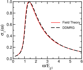
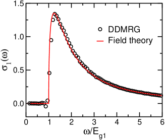
Figure 11: Optical conductivity of the one-dimensional half-filled Hubbard model for $U=3t$. Left panel: DDMRG result calculated on a 128-site lattice using a broadening $\eta=0.1t$ (dashed line) and field-theoretical prediction for the infinite chain [39] broadened with a Lorentzian of width $\eta=0.1t$ (solid line). Right panel: the field-theoretical prediction without broadening (solid line) and the DDMRG result after deconvolution (circles).

4.3 Spectrum in the thermodynamic limit

DDMRG allows us to calculate spectral functions of a large but finite system with a broadening given by the parameter $\eta>0$. To determine the properties of a dynamical spectrum in the thermodynamic limit, one has to analyze the scaling of the corresponding spectra $I_{N,\eta}(\omega)$ as a function of the system size $N$ for vanishing broadening $\eta$

$$I(\omega)=\lim_{\eta\rightarrow 0}\lim_{N\rightarrow\infty}I_{N,\eta}(\omega).$$ (42)

Computing both limits in this equation from numerical results for $I_{N,\eta}(\omega)$ requires a lot of accurate data for different values of $\eta$ and $N$ and can be the source of large extrapolation errors. A much better approach is to use a broadening $\eta(N)>0$ which decreases with increasing $N$ and vanishes in the thermodynamic limit [40]. The dynamical spectrum is then given by $I(\omega)=\lim_{N\rightarrow\infty}I_{N,\eta(N)}(\omega).$ From the existence of both limits in eq. (42) it can be demonstrated that there exists a minimal broadening $\eta_{0}(N)\geq 0$, which converges to zero for $N\rightarrow\infty$, such that this procedure is exact for all functions $\eta(N)$ with $\eta(N)>\eta_{0}(N)$ and $\lim_{N\rightarrow\infty}\eta(N)=0$.

The function $\eta_{0}(N)$ depends naturally on the specific problem studied and can also vary for each frequency $\omega$ considered. For one-dimensional correlated electron systems such as the Hubbard model (1), one finds empirically that a sufficient condition is

$$\eta(N)=\frac{c}{N},$$ (43)

where the constant $c$ is comparable to the effective width of the dynamical spectrum $I(\omega)$, which is finite in such lattice models. This condition has a very simple physical interpretation. The spectral function $I_{N,\eta}(\omega)$ represents the dynamical response of the system over a time period $\sim 1/\eta$ after one has started to apply an external force. Typically, in a lattice model the spectral width is proportional to the velocity of the excitations involved in the system response. Thus the condition (43) means that excitations are too slow to travel the full length $\sim N$ of the system in the time interval $\sim 1/\eta$ and do not “sense” that the system is finite.

An additional benefit of a broadening satisfying the condition (43) is that the finite-system spectrum $I_{N,\eta}(\omega)$ becomes indistinguishable from the infinite-system spectrum with the same broadening $\eta$ for relatively small $N$. Therefore, if one knows a spectral function $I(\omega)$ for an infinite system, its convolution with a Lorentzian of width $\eta$ can be compared directly with the numerical results for the finite-system spectrum $I_{N,\eta}(\omega)$. This is the approach used in fig. 11 (left panel) to compare DDMRG results for a finite lattice with the field-theoretical prediction for an infinite chain.

Finally, an approximation for an infinite-system (continuous) spectrum can be obtained by solving the convolution equation (34) numerically for $I_{A}(\omega^{\prime})$ using the numerical DDMRG data for a finite system on the left-hand side of this equation [55]. Performing such a deconvolution is a ill-conditioned inverse problem, which can only be solved approximately using some assumptions on the spectrum properties like its smoothness. Therefore, the accuracy of deconvolved DDMRG spectra is unknown. In practice, however, one obtains often accurate results as shown in fig. 11 (right panel), where a deconvolved DDMRG spectrum is compared to an exact field-theoretical result.

In summary, the dynamical spectrum of an infinite system can be determined accurately and efficiently from numerical (DDMRG) data for finite-system spectra using a finite-size scaling analysis with a size-dependent broadening $\eta(N)$.

4.4 Application to electron-phonon problems

The DDMRG algorithm described in the previous section can be applied to EP systems such as the Holstein-Hubbard model without modification [56]. It can naturally be combined with the special DMRG techniques for systems with bosonic degrees of freedom which are described in subsect. 3.4. As for ground-state simulations, these special techniques substantially reduce the computational cost for calculating dynamical properties of EP systems. Nevertheless, applications of DDMRG to the Holstein-Hubbard model are significantly more costly than those for comparable purely electronic systems such as the Hubbard model.

As an illustration, we compare DDMRG and ED-KPM (subsubsect. 2.4.2) results for the spectral functions of an eight-site spinless Holstein model in fig. 12. There is an excellent overall agreement between both methods. The observable differences are due to the larger broadening $\eta=0.1t$ used in the DDMRG simulation. This hides the sharpest details of the spectrum like the oscillations which are visible in the KPM spectrum.

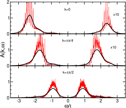
Figure 12: Spectral functions $A(k,\omega)$ (for electron removal, $\omega<0$, and electron injection, $\omega>0$) of the spinless Holstein model at half filling on a 8-site lattice with periodic boundary conditions. The system is in the CDW/Peierls insulating phase ($\omega=0.1t$ and $g=4$). The rapidly oscillating thin lines are the KPM results while the smooth thick line are the DDMRG results with the pseudo-site method. Note that only $|k|\leq\pi/2$ is shown because $A(k\pm\pi,\omega)=A(k,-\omega)$.

A significant difference between both methods is the computational cost. These DDMRG calculations took only 150 CPU hours on an Opteron 244 processor (1.8 GHz) and required less than 300 MBytes of memory. It is thus possible to simulate significantly larger EP systems than this eight-site lattice with DDMRG while this system size is the largest one which can be simulated with exact diagonalization techniques.

Finally, we note that the broadening $\eta=0.1t$ used for the DDMRG results in fig. 12 is one order of magnitude smaller than the value used for a purely electronic systems of comparable size (see fig. 11). It seems that the scaling (43) is not applicable to EP systems. Analytical and numerical investigations will be necessary to determine the function $\eta_{0}(N)$ for EP systems before one can investigate their dynamical properties in the thermodynamic limit using the techniques described in subsect. 4.3.

5 Conclusion

Exact diagonalization and density matrix renormalization group techniques are powerful and versatile exact numerical approaches for investigating the properties of electron-phonon lattice models for strongly correlated (low-dimensional) materials. Thanks to recent developments we can now calculate dynamical quantities which are directly related to experimental techniques used in solid-state spectroscopy and often determine the properties in the thermodynamic limit using a finite-size scaling analysis.

- [1]
- [2] For an overview on several important aspects of strongly correlated electron systems, see Science Vol. 288 Nr. 5465 (2000).
- [3] \BYBishop A.R. \atqueSwanson B.I. \INNovel Electronic Materials: the MX Family. Los Alamos Science211993133.
- [4] \BYHubbard J. \INProc. R. Soc. London, Ser. A2761963238.
- [5] \BYHolstein T. \INAnn. Phys. (N.Y.)81959325; 343.
- [6] Bäuml B., Wellein G. and Fehske H., Phys. Rev. B, 58 (1998) 3663.
- [7] Wellein G., Röder H. and Fehske H., Phys. Rev. B, 53 (1996) 9666.
- [8] Augier D. and Poilblanc D., Eur. Phys. J. B, 1 (1998) 19.
- [9] Sykora S., Hübsch A., Becker K.W., Wellein G. and Fehske H., Phys. Rev. B, 71 (2005) 045112.
- [10] Bonča J., Trugman S.A. and Batistić I., Phys. Rev. B, 60 (1999) 1633.
- [11] Ku L.C., Trugman S.A. and Bonča J., Phys. Rev. B, 65 (2002) 174306.
- [12] Cullum J.K. and Willoughby R.A., Lanczos Algorithms for Large Symmetric Eigenvalue Computations, Volume I & II (Birkhäuser, Boston), 1985.
- [13] Davidson E.R., J. Comput. Phys., 17 (1975) 87.
- [14] Barret R. et al., Templates for the Solution of Linear Systems: Building Blocks for Iterative Methods (SIAM, Philadelphia), 1993.
- [15] Weiße A., Wellein G., Alvermann A. and Fehske H., The kernel polynomial method, Rev. Mod. Phys., 78 (2006) 275, URL http://arXiv.org/abs/cond-mat/0504627.
- [16] Silver R.N. and Röder H., Phys. Rev. E, 56 (1997) 4822.
- [17] Sénéchal D., Perez D. and Pioro-Ladrière M., Phys. Rev. Lett., 84 (2000) 522.
- [18] \BYWhite S.R. \INPhys. Rev. Lett.6919922863; \INPhys. Rev. B48199310345.
- [19] For a recent review, see \BYSchollwöck U. \INRev. Mod. Phys.772005259.
- [20] \BYNoack R.M. \atqueWhite S.R. \TITLEThe Density Matrix Renormalization Group, in \TITLEDensity-Matrix Renormalization, A New Numerical Method in Physics, edited by \NAMEPeschel I., Wang X., Kaulke M. \atqueHallberg K. (Springer, Berlin) 1999, Chap. 2.
- [21] See URL http://alps.comp-phys.org/.
- [22] \BYWilson K.G. \INRev. Mod. Phys.471975773.
- [23] \BYBray J.W. \atqueChui S.T. \INPhys. Rev. B1919794876.
- [24] \BYWhite S.R. \atqueNoack R.M. \INPhys. Rev. Lett.6819923487.
- [25] \BYBursill R.J. \INPhys. Rev. B6019991643.
- [26] \BYCaron L.G. \atqueMoukouri S. \INPhys. Rev. Lett.7619964050; \INPhys. Rev. B561997R8471.
- [27] \BYPeschel I., Kaulke M. \atqueLegeza Ö. \INAnn. Phys. (Leipzig)81999153; \BYPeschel I. \atqueChung M.-C. \INJ. Phys. A3219998419; \BYChung M.-C. \atquePeschel I. \INPhys. Rev. B6220004191; \SAME642001064412.
- [28] \BYBonca J., Gubernatis J.E., Guerrero M., Jeckelmann E. \atqueWhite S.R. \INPhys. Rev. B6120003251.
- [29] \BYJeckelmann E. \INPhys. Rev. Lett.892002236401.
- [30] \BYJeckelmann E. \atqueWhite S.R. \INPhys.Rev B5719986376.
- [31] \BYZhang C., Jeckelmann E. \atqueWhite S.R. \INPhys. Rev. Lett.8019982661.
- [32] \BYZhang C., Jeckelmann E. \atqueWhite S.R. \INPhys. Rev. B60199914092.
- [33] \BYRomero A.H., Brown D.W. \atqueLindenberg K. \INJ. Chem. Phys.10919986540.
- [34] \BYJeckelmann E., Zhang C. \atqueWhite S.R. \INPhys.Rev B6019997950.
- [35] \BYWeiße A., Fehske H., Wellein G. \atqueBishop A.R. \INPhys. Rev. B622000R747.
- [36] \BYWeisse A., Wellein G. \atqueFehske H. \TITLEDensity-Matrix Algorithm for Phonon Hilbert Space Reduction in the Numerical Diagonalization of Quantum Many-Body Systems, in \TITLEHigh Performance Computing in Science and Engineering’01, edited by \NAMEKrause E. \atqueJäger W. (Springer, Berlin) 2002, pp 131.
- [37] \BYFriedman B. \INPhys Rev. B6120006701.
- [38] \BYKuzmany H. \TITLESolid-State Spectroscopy (Springer, Berlin) 1998.
- [39] \BYJeckelmann E., Gebhard F. \atqueEssler F.H.L \INPhys. Rev. Lett.8520003910.
- [40] \BYJeckelmann E. \INPhys. Rev. B662002045114.
- [41] \BYWhite S.R. \atqueHuse D.A. \INPhys. Rev. B4819933844.
- [42] \BYMcCulloch I.P. \atqueGulácsi M. \INEurophys. Lett.572002852.
- [43] \BYRamasesha S., Pati S.K., Krishnamurthy H.R., Shuai Z. \atqueBrédas J.L. \INPhys. Rev. B5419967598.
- [44] \BYBoman M. \atqueBursill R.J. \INPhys. Rev. B57199815167.
- [45] \BYRamasesha S., Pati S.K., Shuai Z. \atqueBrédas J.L. in \TITLEAdvances in Quantum Chemistry, Volume 38 (Academic Press) 2001, pp. 121-215.
- [46] \BYDaul S. \atqueNoack R.M. \INPhys. Rev. B5819982635.
- [47] \BYHallberg K.A. \INPhys. Rev. B521995R9827.
- [48] \BYZhang C. \TITLENumerical Study of the One-Dimensional Holstein Model (Ph.D. thesis, University of California at Irvine) 1999.
- [49] \BYPati S.K., Ramasesha S., Shuai Z. \atqueBrédas J.L. \INPhys. Rev. B59199914827; \BYRamasesha S., Pati S.K., Krishnamurthy H.R., Shuai Z. \atqueBrédas J.L. \INSynth. Met.8519971019.
- [50] \BYKühner T.D. \atqueWhite S.R. \INPhys. Rev B601999335.
- [51] \BYEssler F.H.L, Jeckelmann E. \atqueGebhard F. \INPhys. Rev. B642001125119.
- [52] \BYJeckelmann E. \INPhys. Rev. B672003075106.
- [53] \BYBenthien H., Gebhard B. \atqueJeckelmann E. \INPhys. Rev. Lett.922004256401.
- [54] \BYBenthien H. \TITLEDynamical Properties of Quasi One-Dimensional Correlated Electron Systems (Ph.D. thesis, University of Marburg, Germany) 2005.
- [55] \BYNishimoto S. \atqueJeckelmann E. \INJ. Phys. Condens. Matter162004613.
- [56] \BYHager G., Jeckelmann E., Fehske H. \atqueWellein G. \TITLEExact Numerical Treatment of Finite Quantum Systems using Leading-Edge Supercomputers, in \TITLEModelling, Simulation and Optimization of Complex Processes, edited by \NAMEBock H.G., Kostina E., Phu H.-X. \atqueRannacher R. (Springer, Heidelberg) 2005, pp. 165.