0pt0.4pt 0pt0.4pt 0pt0.4pt

Integrable models for asymmetric Fermi superfluids: Emergence of a new exotic pairing phase

Abstract

We introduce an exactly-solvable model to study the competition between the Larkin-Ovchinnikov-Fulde-Ferrell (LOFF) and breached-pair superfluid in strongly interacting ultracold asymmetric Fermi gases. One can thus investigate homogeneous and inhomogeneous states on an equal footing and establish the quantum phase diagram. For certain values of the filling and the interaction strength, the model exhibits a new stable exotic pairing phase which combines an inhomogeneous state with an interior gap to pair-excitations. It is proven that this phase is the exact ground state in the strong coupling limit, while numerical examples in finite lattices show that also at finite interaction strength it can have lower energy than the breached-pair or LOFF states.

Superconducting and Fermi superfluid phenomena have been a subject of fascination since their discovery. Both phenomena are direct macroscopic-scale manifestations of quantum physics, with the electric charge of their relevant microscopic constituents being the crucial factor differentiating them. Interest in their various fundamental aspects has increased recently because advances in the field of ultracold atomic Fermi gases Regal ; becbcs are leading to new experimental probes to investigate unexplored territory, with consequences in condensed matter as well as high energy physics (e.g., the physics in the core of neutron stars).

Of particular importance is the nature of their ground states (GSs) under various external conditions since novel thermodynamic phases might show up. The present manuscript studies the relative vacuum stability of a two-species fermion gas as a function of the pairing interaction strength $g$ and different species population. Without loss of generality we denote the two species as $a$ and $b$ with densities $\rho_{a(b)}$. Differences among the two species could be related to their masses $m_{a(b)}$, spin or hyperfine states. Asymmetry, in general, makes pairing less favorable and questions about the nature of the resulting competing phases might arise. To this end, we introduce a model system that will prove to be exactly solvable and which displays the competition between the Larkin-Ovchinnikov-Fulde-Ferrell (LOFF) loff , breached-pair (or Sarma) sarma ; liu , deformed Fermi-surface superfluid sedra , and segregated phases bedaque . Its quantum phase diagram as a function of the asymmetry density $\delta\rho=(\rho_{a}-\rho_{b})/(\rho_{a}+\rho_{b})$ and the coupling strength $g$ has been recently studied, at the mean-field level, in the one-channel phase and two-channel models phase2 . In our exact solution, albeit in a finite-size lattice, we find different regimes of stability for these various phases. A key result is the prediction of a new exotic inhomogeneous phase characterized by a particular center-of-mass momentum of the condensed pairs. This phase is the exact GS in the large-$g$ limit.

Consider $N_{a}$ and $N_{b}$ fermionic atoms confined to a $D$-dimensional box of volume $V$, i.e. $\rho_{a(b)}=N_{a(b)}/V$, with periodic boundary conditions and $g<0$. (The exact solvability of the problem is not restricted to these latter conditions but for notational convenience we will specialize to this case). The following model Hamiltonian contains the right ingredients to study the competition between the various phases

$$H=\sum_{\mathbf{k}}(\varepsilon_{\mathbf{k}}^{a}\ n^{a}_{\mathbf{k}}+\varepsilon_{\mathbf{k}}^{b}\ n^{b}_{\mathbf{k}})+2g\sum_{\mathbf{k},\mathbf{k}^{\prime}}a_{\mathbf{k}+\mathbf{Q}}^{\dagger}b_{-\mathbf{k}}^{\dagger}b_{-\mathbf{k}^{\prime}}^{\;}a_{\mathbf{k}^{\prime}+\mathbf{Q}}^{\;},$$ (1)

where $a_{\mathbf{k}}^{\dagger}$($b_{\mathbf{k}}^{\dagger}$) creates a particle of type $a$($b$) with momentum $\mathbf{k}$ and $n^{a}_{\mathbf{k}}=a_{\mathbf{k}}^{\dagger}a^{\;}_{\mathbf{k}}$, $n^{b}_{\mathbf{k}}=b_{\mathbf{k}}^{\dagger}b^{\;}_{\mathbf{k}}$. The pairing interaction scatters pairs with center-of-mass momentum $\mathbf{Q}$ and “band” energies $\varepsilon_{\mathbf{k}}^{\alpha}=\epsilon_{\mathbf{k}}/2m_{\alpha}$ ($\alpha=a,b$), with $\epsilon_{\mathbf{k}}$ representing an arbitrary dispersion (including a non-rotational-invariant one sedra ).

The quantum integrability and exact solvability of the Hamiltonian (1) can be derived using an $su(2)$ algebra

$${\tau}_{\mathbf{k},\mathbf{Q}}^{+}=a_{\mathbf{k}+\mathbf{Q}}^{\dagger}b_{-\mathbf{k}}^{\dagger}=(\tau_{\mathbf{k},\mathbf{Q}}^{-})^{\dagger}\ ,\ {\tau}_{\mathbf{k},\mathbf{Q}}^{z}=\frac{1}{2}(n^{a}_{\mathbf{k}+\mathbf{Q}}+n^{b}_{-\mathbf{k}}-1)\ ,$$ (2)

and a second, independent, realization of $su(2)$

$${S}_{\mathbf{k},\mathbf{Q}}^{+}=a_{\mathbf{k}+\mathbf{Q}}^{\dagger}b_{-\mathbf{k}}^{\;}=(S_{\mathbf{k},\mathbf{Q}}^{-})^{\dagger}\ ,\ {S}_{\mathbf{k},\mathbf{Q}}^{z}=\frac{1}{2}(n^{a}_{\mathbf{k}+\mathbf{Q}}-n^{b}_{-\mathbf{k}})\ .$$ (3)

These two mutually commuting algebras are often referred to as charge and spin $su(2)$ realizations, respectively. Using the algebraic techniques of the Richardson-Gaudin model NB , one can write down a complete set of integrals of motion $R^{\sf{T}}_{\mathbf{k},\mathbf{Q}}$, with $[R^{\sf{T}}_{\mathbf{k},\mathbf{Q}},R^{{\sf{T}}^{\prime}}_{\mathbf{k}^{\prime},\mathbf{Q}}]=0$ (for ${\sf{T}},{\sf{T}}^{\prime}=\tau,S$): $R_{\mathbf{k},\mathbf{Q}}^{{\sf{T}}}={\sf{T}}_{\mathbf{k},\mathbf{Q}}^{z}+2g_{\sf{T}}\sum_{\mathbf{k}^{\prime}(\neq\mathbf{k})}X_{\mathbf{k}\mathbf{k}^{\prime}}^{\sf{T}}\ \vec{{\sf{T}}}_{\mathbf{k},\mathbf{Q}}\cdot\vec{{\sf{T}}}_{\mathbf{k}^{\prime},\mathbf{Q}}$, where $X_{\mathbf{k}\mathbf{k}^{\prime}}^{\sf{T}}=1/(\eta^{\sf{T}}_{\left(\mathbf{k},\mathbf{Q}\right)}-\eta^{\sf{T}}_{\left(\mathbf{k}^{\prime},\mathbf{Q}\right)})$, with arbitrary functions $\eta^{\sf{T}}$ depending upon $\mathbf{k}$ and $\mathbf{Q}$, and $g_{\sf{T}}$ are the coupling constants. Their complete set of eigenvectors are of the form

$$\left|\Psi\right\rangle=\prod\limits_{\ell=1}^{M_{\sf{T}}}\left(\sum_{\mathbf{k}}\frac{1}{2\eta_{\left(\mathbf{k},\mathbf{Q}\right)}^{\sf{T}}-E_{\ell}^{\sf{T}}}\ {\sf{T}}_{\mathbf{k},\mathbf{Q}}^{+}\right)\left|\nu^{\sf{T}}\right\rangle,$$ (4)

where $\left|\nu^{\sf{T}}\right\rangle\equiv$ $\prod\limits_{\mathbf{k}}\left|\nu_{\mathbf{k},\mathbf{Q}}^{\sf{T}}\right\rangle$ is a quasispin vacuum state defined by ${\sf{T}}_{\mathbf{k},\mathbf{Q}}^{-}\left|\nu^{\sf{T}}\right\rangle=0$, and ${\sf{T}}_{\mathbf{k},\mathbf{Q}}^{z}\left|\nu^{\sf{T}}\right\rangle=d_{\mathbf{k},\mathbf{Q}}^{\sf{T}}\left|\nu^{\sf{T}}\right\rangle$, with $d_{\mathbf{k},\mathbf{Q}}^{\sf{T}}=(2\nu^{\sf{T}}_{\mathbf{k},\mathbf{Q}}-\Omega_{\mathbf{k},\mathbf{Q}})/4$, $\Omega_{\mathbf{k},\mathbf{Q}}=2$, and the seniority quantum number $\nu_{\mathbf{k},\mathbf{Q}}^{\sf{T}}=1,0$, which for the $su(2)$ pair algebra (2) counts the number of unpaired fermions. The complex spectral parameters $E_{\ell}^{\sf{T}}$ satisfy the set of non-linear equations

$$\frac{1}{4g_{\sf{T}}}-\sum_{\mathbf{k}}\frac{d_{\mathbf{k},\mathbf{Q}}^{\sf{T}}}{2\eta^{\sf{T}}_{\left(\mathbf{k},\mathbf{Q}\right)}-E_{\ell}^{\sf{T}}}+\sum_{m\left(\neq\ell\right)}\frac{1}{E_{\ell}^{\sf{T}}-E_{m}^{\sf{T}}}=0\ .$$ (5)

To simplify matters, and because our goal is to show exact solvability of (1), we will only consider dynamics in the charge space (i.e., $g_{S}=0$, $g_{\tau}=g$, dropping the label ${\sf{T}}$). The total number of atoms is $N=N_{a}+N_{b}=2M+\nu$, where $M$ is the number of atom pairs and $\nu$ the number of unpaired ones. Consider now the linear combination $H_{\tau}=2\sum_{\mathbf{k}}\eta_{\left(\mathbf{k},\mathbf{Q}\right)}R_{\mathbf{k},\mathbf{Q}}^{\tau}=\sum_{\mathbf{k}}2\eta_{\left(\mathbf{k},\mathbf{Q}\right)}\tau_{\mathbf{k},\mathbf{Q}}^{z}+2g\sum_{\mathbf{k},\mathbf{k}^{\prime}}\tau_{\mathbf{k},\mathbf{Q}}^{+}\tau_{\mathbf{k}^{\prime},\mathbf{Q}}^{-}+C$, where $C=3g\sum_{\mathbf{k}}d_{\mathbf{k},\mathbf{Q}}+g\left(N-L\right)^{2}/2-g\left(N-L\right)$. Comparing $H_{\tau}$ with (1) we immediately see that they differ in the kinetic term. Making use of the spin $su(2)$ algebra by adding a term of the form $2\sum_{\mathbf{k}}\xi_{(\mathbf{k},\mathbf{Q})}S^{z}_{\mathbf{k},\mathbf{Q}}$, it leads to (up to an irrelevant constant)

$$H = \sum_{\mathbf{k}}[(\eta_{\left(\mathbf{k},\mathbf{Q}\right)}+\xi_{\left(\mathbf{k},\mathbf{Q}\right)})n^{a}_{\mathbf{k}+\mathbf{Q}}+(\eta_{\left(\mathbf{k},\mathbf{Q}\right)}-\xi_{\left(\mathbf{k},\mathbf{Q}\right)})n^{b}_{-\mathbf{k}}]$$ (6)

$$+ 2g\sum_{\mathbf{k},\mathbf{k}^{\prime}}\tau_{\mathbf{k},\mathbf{Q}}^{+}\tau_{\mathbf{k}^{\prime},\mathbf{Q}}^{-}.$$

Identifying $\eta_{\left(\mathbf{k},\mathbf{Q}\right)}=\frac{1}{2}[\varepsilon^{a}_{\mathbf{k}+\mathbf{Q}}+\varepsilon^{b}_{-\mathbf{k}}]$, and $\xi_{\left(\mathbf{k},\mathbf{Q}\right)}=\frac{1}{2}[\varepsilon^{a}_{\mathbf{k}+\mathbf{Q}}-\varepsilon^{b}_{-\mathbf{k}}]$, we get the Hamiltonian of Eq. (1), after constraining the vectors $\mathbf{k}+\mathbf{Q}$ and $\mathbf{k}$ to be in the same set. The eigenvalue $E$ corresponding to the solutions of Eqs. (5) are given by

$$E=\sum_{\mathbf{k}}\left(\varepsilon^{a}_{\mathbf{k}+\mathbf{Q}}\nu^{a}_{\mathbf{k}+\mathbf{Q}}+\varepsilon^{b}_{-\mathbf{k}}\nu^{b}_{-\mathbf{k}}\right)+\sum_{\ell}E_{\ell},$$ (7)

where $\nu^{\alpha}_{\mathbf{k}}$ denotes the number of unpaired $\alpha$ particles in the state with momentum $\mathbf{k}$. The space dimensionality of the problem enters through the band dispersion $\varepsilon_{\mathbf{k}}^{\alpha}$, and the effective degeneracies $d_{\mathbf{k},\mathbf{Q}}$ in the exact solution (5). The latter are in turn defined by $\eta_{\left(\mathbf{k},\mathbf{Q}\right)}$. Assuming space-inversion symmetry ($\varepsilon_{\mathbf{k}}^{\alpha}=\varepsilon_{-\mathbf{k}}^{\alpha}$), the degeneracies $\Omega_{\mathbf{k},\mathbf{Q}}$ count the number of states [$\mathbf{k},\mathbf{Q}$] with the same value of $\eta_{\left(\mathbf{k},\mathbf{Q}\right)}$.

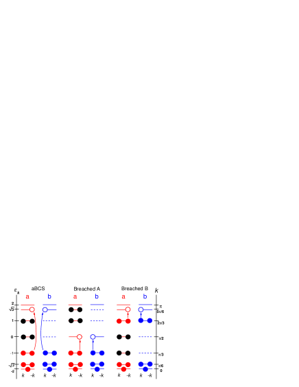
Figure 1: Three $\mathbf{Q}={\bf 0}$ configurations, asymmetric BCS (aBCS), breached A, and breached B, as described in the text for a $D=1$ lattice with 12 sites, $N_{a}=9$ and $N_{b}=5$ atoms. The left vertical axis displays the single-particle energies $\varepsilon_{\mathbf{k}}^{\alpha}=-2\cos\mathbf{k}$ ($\alpha=a,b$) while the right one shows the corresponding momenta $\mathbf{k}$. An allowed pair-scattering process is indicated in each case with arrows.

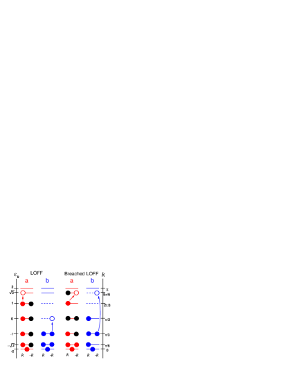
Figure 2: Two possible $\mathbf{Q}=\pi/3$ configurations. The first one (LOFF) corresponds to a Fermi sea. A possible pair-scattering process is indicated with arrows. We show a breached LOFF configuration as a second example. The $\mathbf{k}$ momentum values are the same as in LOFF.

Our exactly-solvable model is valid for arbitrary $\mathbf{Q}$ values. The $\mathbf{Q}={\bf 0}$ limit restores the homogeneous BCS phase giving rise to a breached-pair phase in terms of ${\bf 0}$-momentum pairs, while a finite value of $\mathbf{Q}$ gives rise to the LOFF phase with $\mathbf{Q}$-momentum pairs. For an asymmetric system with an excess of the $a$ species ($N_{a}>N_{b}$), the atoms fill the lowest states up to $\mathbf{k}_{F}^{b}$ with $|\mathbf{k}_{F}^{a}|>|\mathbf{k}_{F}^{b}|$ at weak coupling. When the interaction is switched on, several possible states compete to determine the absolute GS. The position of the unpaired atoms, defining the seniority quantum numbers $\nu_{\mathbf{k},\mathbf{Q}}$, block the available states from scattering pairs of atoms effectively reducing the degeneracies to $d_{\mathbf{k},\mathbf{Q}}$. When $\mathbf{Q}={\bf 0}$ the equations reduce to the well-known Richardson model with blocked states RichN ; NB . In general, configurations are identified by their $g\rightarrow 0$ limit, with specific pair and seniority occupations. They can be categorized as follows:

• asymmetric BCS (aBCS): $\mathbf{Q}={\bf 0}$, $a$ and $b$ particles fill their lowest orbitals up to their corresponding Fermi levels.

• breached A: same as aBCS, but the unpaired $a$ particles move up in energy such that pairing correlations can develop around $\mathbf{k}_{F}^{b}$.

• breached B: same as aBCS, but the unpaired $a$ particles move down in energy such that pairing correlations can develop around $\mathbf{k}_{F}^{a}$.

• LOFF: finite $\mathbf{Q}$, $a$ and $b$ particles fill their lowest orbitals up to their corresponding Fermi levels.

• breached LOFF: finite $\mathbf{Q}$, but now some of the unpaired $a$ particles move to allow more pairing correlations.

We illustrate some of these states by using a $D=1$ lattice with $L=12$ modes as an example. In Fig. 1 we show the level scheme for a system with $N_{a}=9$ and $N_{b}=5$. In the first column, labeled aBCS, the excess of $a$ atoms occupy the states between $\mathbf{k}_{F}^{b}$ and $\mathbf{k}_{F}^{a}$ completely blocking these states. The corresponding $b$ states are represented by a dash line. Pair scattering can only occur between states below $\mathbf{k}_{F}^{b}$ and states above $\mathbf{k}_{F}^{a}$, as indicated in the figure. It is worth noting that the excess of $a$ atoms could be located in any configuration in $\mathbf{k}$-space. In the second column we display a breached-pair superfluid state sarma ; liu ; bedaque (Breached A) where the unpaired $a$ atoms are promoted to higher-energy states to leave some space around $\mathbf{k}_{F}^{b}$ for pairing. A possible pair-scattering process is indicated in the figure. Alternatively, the blocked states could be moved down for the pair scattering to take place around $\mathbf{k}_{F}^{a}$ as shown in the third column of the same figure (Breached B). The relative stability of each one of these possible states will depend upon the competition between the kinetic energy and the pairing interaction.

Figure 2 displays two examples of a LOFF state configuration. Here we assume a momentum $\mathbf{Q}$ that exactly matches the two Fermi energies ($\mathbf{Q}=\mathbf{k}_{F}^{a}-\mathbf{k}_{F}^{b}=\pi/3$). In the first example, corresponding to the first two columns of Fig. 2, the atoms occupy the lowest single-particle energies $\varepsilon_{\mathbf{k}}^{\alpha}$ defining a configuration which is expected to be the lowest LOFF state at weak coupling. The numbers within the circles indicate the $\mathbf{Q}=\pi/3$ momentum pairs. The unpaired $a$ atoms, displayed with a black circle, block the corresponding states of the $b$ atoms. A possible breached LOFF configuration is shown as a second example.

We will now explore the competition between the possible phases in a numerical example for $D=2$. We assume a square lattice with dispersion $\varepsilon_{\mathbf{k}}^{\alpha}=-2(\cos(k_{x})+\cos(k_{y}))$, with units chosen such that $k_{x}$ and $k_{y}$ are multiples of $2\pi/L$, where $L$ is the linear size of the lattice. Being the dispersion equal for both atomic species, we are excluding an asymmetry in the masses or a deformed Fermi surface. Preliminary results for asymmetric masses do not show qualitative differences with the results presented below, except that for $m_{a}>m_{b}$ breached A will be more stable than breached B because particles of type $a$ will require less kinetic energy to shift to higher momenta than particles of type $b$.

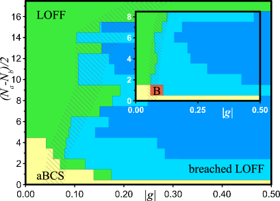
Figure 3: Quantum phase diagram for a $6\times 6$ lattice at half filling; the inset displays the quarter-filling case (aBCS: yellow, LOFF: green, breached B: red, breached LOFF: blue, dark blue for $\mathbf{Q}=(\pi,\pi)$). The shaded area indicates the transition from the normal to the superfluid phase elec .

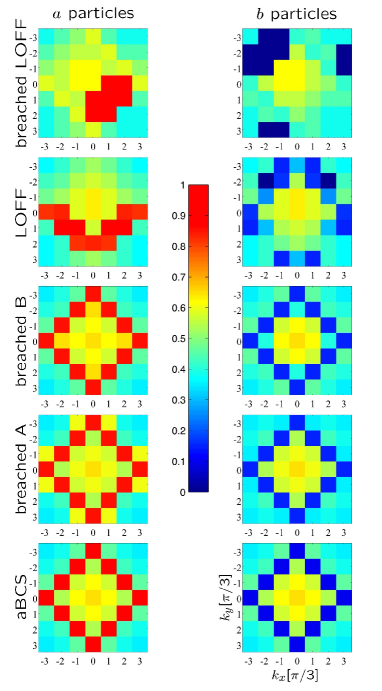
Figure 4: Occupation numbers in momentum space for various configurations with particle numbers $N_{a}=22$ and $N_{b}=14$, at $g=-0.5$, for a $6\times 6$ lattice (LOFF:$\mathbf{Q}=(\pi/3,0)$; breached LOFF:$\mathbf{Q}=(\pi/3,\pi/3)$). Occupation numbers for the unpaired particles have been symmetrized over all possible orientations.

We discuss first the limiting cases of a very weak or very strong pairing interaction. If the interaction strength $g$ is much smaller than the level spacing, then the full problem reduces to a pairing problem for each level separately, with the coupling between levels entering at order $g^{2}$. The leading order is the single-particle energy. This means that the GS fills the lowest single-particle orbitals up to the Fermi levels of species $a$ and $b$, respectively. This leaves no room for the breached-pair phase in the GS. aBCS and LOFF are degenerate to leading order. This degeneracy is lifted at first or second order in $g$. The pairing interaction favors open shells, hence it prefers a non-zero value of $\mathbf{Q}$ when the valence shell is completely filled, while it might prefer $\mathbf{Q}={\bf 0}$ for open valence shells. For the $6\times 6$ model studied here, we found that aBCS dominates the weak limit for $N_{a}-N_{b}<4$ at quarter filling and for $N_{a}-N_{b}<10$ at half filling.

In the strong-coupling limit one can expand Eq. (5) in terms of $g^{-1}$. In this way, the asymptotic GS of (1) can be analytically determined Yuzba03 . The resulting GS energy is given by

$$E_{0} = -2gN_{b}(2\Omega+1-N_{b})+\sum_{\mathbf{k}}\varepsilon_{\mathbf{k}}^{a}\nu_{\mathbf{k}}^{a}$$ (8)

$$+ 2N_{b}\ \frac{\sum_{\mathbf{k}}d_{\mathbf{k},\mathbf{Q}}\ \eta_{(\mathbf{k},\mathbf{Q})}}{\sum_{\mathbf{k}}d_{\mathbf{k},\mathbf{Q}}}+{\mathcal{O}(g^{-1})},$$

with $\Omega=\sum_{\mathbf{k}}\Omega_{\mathbf{k},\mathbf{Q}}$. Upon inspection one finds that for the lattice model considered here, the lowest possible value for $E_{0}$ will occur when $\mathbf{Q}=(\pi,\pi)$. In that case all $\eta_{(\mathbf{k},\mathbf{Q})}$ vanish, and the first line of Eq. (8) becomes an exact expression with the excess $a$ atoms occupying the lowest single-particle states. One can describe this regime as an extreme breached LOFF state. This result is exact in the limit of $|g|$ much larger than the bandwidth, which is an unphysical assumption. However, it indicates that at some finite value of $g$ a transition to an exotic inhomogeneous phase must occur, combining a breached configuration with a non-zero value for $\mathbf{Q}$. We find such configurations to have a lower energy than the aBCS, breached A or B or LOFF configurations at interaction strengths as weak as $g=-0.1$, which might be realizable in a physical setting.

We have studied model (1) numerically on a $6\times 6$ lattice, with 18 (quarter-filled) or 36 (half-filled) particles, distributed over $a$ and $b$ states. Finding the optimal configuration for the unpaired particles turned out to be highly non-trivial because of the large number of possibilities. We addressed this problem using a quantum Monte Carlo technique Romb05 that provided a number of candidate GS configurations for various values of $g$ and $\mathbf{Q}$. Starting from the $g=0$ configurations, the solution of Eq. (5) was then obtained by slowly increasing the value of $g$, and by applying the iteration techniques explained in Ref. Romb04 . In this way we evaluated the exact energies for each configuration up to $g=-0.5$, and we were able to determine the GS and the exact transition points. One can see in Fig. 3 that exotic configurations such as LOFF or breached LOFF can have a lower energy than the aBCS state. There is a subtle competition between LOFF and the various breached BCS states, and both phenomena appear simultaneously in the emergent breached-LOFF regime that dominates the phase diagram at larger asymmetries and interaction strengths. The recently observed Ket normal state region at weak coupling could be qualitatively determined using the techniques discussed in elec . Our approach also allows computation of the occupation numbers in momentum space. They are derived from the integrals of motion using the Hellman-Feynman theorem. Figure 4 shows results for a selected number of configurations, corresponding to the lowest-lying states of the half-filled model at $N_{a}-N_{b}=8$, to illustrate the aBCS, breached A and B, LOFF and breached LOFF phases at $g=-0.5$.

In summary, we presented a one-channel exactly-solvable model that admits several homogeneous and inhomogeneous phases depending upon the relative strength between kinetic and pairing interactions, and the difference in the number of atomic species (given a fixed total number of atoms). The inhomogeneous phases (LOFF) show up as soon as the difference in Fermi momentum between the two species becomes commensurate with the unit lattice momentum. A most significant result is the prediction of a new exotic phase which combines pairs with definite momentum and breached superfluidity/superconductivity, that we dubbed breached LOFF. We expect this new phase to be the stable ground state at large interaction strengths for fixed, asymmetric particle numbers. These phases can be experimentally differentiated in time-of-flight measurements of the molecular velocity, after sweeping the system through the BCS-to-BEC crossover region Regal ; becbcs . The momentum distribution of unpaired fermions may distinguish the various exotic phases discussed here. The present analysis can also be extended to a two-channel integrable model with the explicit treatment of the Feshbach resonance phase2 in a similar way as in Ref. AtMol .

We acknowledge discussions with J. Carlson, W. V. Liu, C. Lobo, S. Reddy and D. Van Neck. JD, SR and KVH acknowledge financial support from the Spanish DGI under grant BFM2003-05316-C02-02, and the FWO - Flanders.

References

- (1) C. A. Regal, M. Greiner, and D. S. Jin, Phys. Rev. Lett. 92, 040403 (2004); M. W. Zwierlein et. al, Phys. Rev. Lett. 92, 120403 (2004).
- (2) G. Ortiz and J. Dukelsky, Phys. Rev. A 72, 043611 (2005).
- (3) A. I. Larkin and Yu. N. Ovchinnikov, Sov. Phys. JETP 20, 762 (1965); P. Fulde and R. A. Ferrell, Phys. Rev. 135, A550 (1964).
- (4) G. Sarma, J. Phys. Chem. Solids 24, 1029 (1963).
- (5) W. V. Liu and F. Wilczek, Phys. Rev. Lett. 90, 047002 (2003).
- (6) H. Muther, and A. Sedrakian, Phys. Rev. Lett. 88, 252503 (2002).
- (7) P. Bedaque et al., Phys. Rev. Lett. 91, 247002 (2003).
- (8) A. Sedrakian et al., Phys. Rev. A 72 013613(2005); C. -H. Pao et al., Phys. Rev. B 73, 132506 (2006); D. T. Son, and M. A. Stephanov, cond-mat/0507586; K. Yang, cond-mat/0508484.
- (9) D. E. Sheehy, and L. Radzihovsky, Phys. Rev. Lett. 96, 060401 (2006).
- (10) J. Dukelsky et al., Rev. Mod. Phys. 76, 643 (2004); G. Ortiz et al., Nucl. Phys. B 707, 421 (2005).
- (11) R. W. Richardson, Phys. Lett. 3, 277 (1963); Nucl. Phys. 52, 221 (1964).
- (12) R. W. Richardson, J. Math. Phys. 18, 1802 (1977); E.A. Yuzbashyan, A.A. Baytin, and B.L. Altshuler, Phys. Rev. B 68, 214509 (2003).
- (13) S. M. A. Rombouts, K. Van Houcke, and L. Pollet, Phys. Rev. Lett. 96 180603 (2006).
- (14) S. Rombouts, D. Van Neck, and J. Dukelsky, Phys. Rev. C 69, 061303 (2004).
- (15) M. W. Zwierlein et al., Science 311, 492 (2006); G. B. Partridge et al., ibid. 311, 503 (2006).
- (16) J. Dukelsky et al., Phys. Rev. Lett. 88, 062501 (2002).
- (17) J. Dukelsky et al., Phys. Rev. Lett. 93, 050403 (2004).