Spin-3 Chromium Bose-Einstein Condensates

Abstract

We analyze the physics of spin-3 Bose-Einstein condensates, and in particular the new physics expected in on-going experiments with condensates of Chromium atoms. We first discuss the ground-state properties, which, depending on still unknown Chromium parameters, and for low magnetic fields can present various types of phases. We also discuss the spinor-dynamics in Chromium spinor condensates, which present significant qualitative differences when compared to other spinor condensates. In particular, dipole-induced spin relaxation may lead for low magnetic fields to transfer of spin into angular momentum similar to the well-known Einstein-de Haas effect. Additionally, a rapid large transference of population between distant magnetic states becomes also possible.

Within the very active field of ultra cold atomic gases, multicomponent (spinor) Bose-Einstein condensates (BECs) have recently attracted a rapidly growing attention. Numerous works have addressed the rich variety of phenomena revealed by spinor BEC, in particular in what concerns ground-state and spin dynamics Ho98 ; Ohmi98 ; Law98 ; Koashi00 ; Ciobanu00 ; Koashi00b ; Pu01 ; You04 ; Ho00b ; Hall98 ; Stenger98 ; Barret01 ; Schmaljohann04 ; Chang04 ; Kuwamoto04 ; Wheeler04 ; Higbie05 ; Widera05 . The first experiments on spinor BEC were performed at JILA using mixtures of ⁸⁷Rb BEC in two magnetically confined internal states (spin-$1/2$ BEC) Hall98 . Optical trapping of spinor condensates was first realized in spin-$1$ Sodium BEC at MIT Stenger98 constituting a major breakthrough since, whereas magnetic trapping confines the BEC to weak-seeking magnetic states, an optical trap enables confinement of all magnetic substates. In addition, the atoms in a magnetic substate can be converted into atoms in other substates through interatomic interactions. Hence, these experiments paved the way towards the above mentioned fascinating phenomenology originating from the spin degree of freedom. Various experiments have been realized since then in spin-$1$ BEC, in particular in ⁸⁷Rb in the $F=1$ manifold. It has been predicted that spin-$1$ BEC can present just two different ground states phases, either ferromagnetic or polar Ho98 . In the case of $F=1$ ⁸⁷Rb it has been shown that the ground-state presents a ferromagnetic behavior Schmaljohann04 ; Chang04 ; Klausen01 . These analyses have been recently extended to spin-$2$ BEC, which presents an even richer variety of possible ground-states, including in addition the so-called cyclic phases Ciobanu00 ; Koashi00b . Recent experiments have shown a behavior compatible with a polar ground-state, although in the very vicinity of the cyclic phase Schmaljohann04 ; Klausen01 . Recently, spin dynamics has attracted a major interest, revealing the fascinating physics of the coherent oscillations between the different components of the manifold Barret01 ; Schmaljohann04 ; Chang04 ; Kuwamoto04 ; Wheeler04 ; Higbie05 .

Very recently, a Chromium BEC (Cr-BEC) has been achieved at Stuttgart University Griesmaier05 . Cr-BEC presents fascinating new features when compared to other experiments in BEC. On one hand, since the ground state of ⁵²Cr is ⁷S₃, Cr-BEC constitutes the first accessible example of a spin-3 BEC. We show below that this fact may have very important consequences for both the ground-state and the dynamics of spinor Cr-BEC. On the other hand, when aligned into the state with magnetic quantum number $m=\pm 3$, ⁵²Cr presents a magnetic moment $\mu=6\mu_{B}$, where $\mu_{B}$ is the Bohr magneton. This dipolar moment should be compared to alkali atoms, which have a maximum magnetic moment of $1\mu_{B}$, and hence $36$ times smaller dipole-dipole interactions. Ultra cold dipolar gases have attracted a rapidly growing attention, in particular in what concerns its stability and excitations Dipoles . The interplay of the dipole-dipole interaction and spinor-BEC physics has been also considered Pu01 ; You04 . Recently, the dipolar effects have been observed for the first time in the expansion of a Cr-BEC Stuhler05 .

This Letter analyzes spin-3 BEC, and in particular the new physics expected in on-going experiments in Cr-BEC. After deriving the equations that describe this system, we focus on the ground-state, using single-mode approximation (SMA), showing that various phases are possible, depending on the applied magnetic field, and the (still unknown) value of the $s$-wave scattering length for the channel of total spin zero. This phase diagram presents certain differences with respect to the diagram first worked out recently by Diener and Ho Diener05 . In the second part of this Letter, we discuss the spinor dynamics, departing from the SMA. The double nature of Cr-BEC as a spin-3 BEC and a dipolar BEC is shown to lead to significant qualitative differences when compared to other spinor BECs. The larger spin can allow for fast population transfer from $m=0$ to $m=\pm 3$ without a sequential dynamics as in $F=2$ ⁸⁷Rb Schmaljohann04 . In addition, dipolar relaxation violates spin conservation, leading to rotation of the different components, resembling the well-known Einstein-de Haas (EH) effect Einstein15 .

In the following we consider an optically trapped Cr-BEC with $N$ particles. The Hamiltonian regulating Cr-BEC is of the form $\hat{H}=\hat{H}_{0}+\hat{V}_{sr}+\hat{V}_{dd}$. The single-particle part of the Hamiltonian, $\hat{H}_{0}$, includes the trapping energy and the linear Zeeman effect (quadratic Zeeman effect is absent in Cr-BEC), being of the form

$$\hat{H}_{0}=\int d{\bf r}\sum_{m}\hat{\psi}_{m}^{\dagger}({\bf r})\left[\frac{-\hbar^{2}}{2M}\nabla^{2}+U_{trap}({\bf r})+pm\right]\hat{\psi}_{m}({\bf r}),$$ (1)

where $\hat{\psi}_{m}^{\dagger}$ ($\hat{\psi}_{m}$) is the creation (annihilation) operator in the $m$ state, $M$ is the atomic mass, and $p=g\mu_{B}B$, with $g=2$ for ⁵²Cr, and $B$ is the applied magnetic field.

The short-range (van der Waals) interactions are given by $\hat{V}_{sr}$. For any interacting pair with spins ${\bf S}_{1,2}$, $\hat{V}_{sr}$ conserves the total spin, $S$, and is thus described in terms of the projector operators on different total spins $\hat{\cal P}_{S}$, where $S=0$, $2$, $4$, and $6$ (only even $S$ is allowed)Ho98 :

$$\hat{V}_{sr}=\frac{1}{2}\int d{\bf r}\sum_{S=0}^{6}g_{S}\hat{\cal P}_{S}({\bf r}),$$ (2)

where $g_{S}=4\pi\hbar^{2}a_{S}/M$, and $a_{S}$ is the $s$-wave scattering length for a total spin $S$. Since ${\bf S}_{1}\cdot{\bf S}_{2}=(S^{2}-S_{1}^{2}-S_{2}^{2})/2$, then $\sum_{S}\hat{\cal P}_{S}({\bf r})=:\hat{n}^{2}({\bf r}):$, $\sum_{S}\lambda_{S}\hat{\cal P}_{S}({\bf r})=:\hat{F}^{2}({\bf r}):$, and $\sum_{S}\lambda_{S}^{2}\hat{\cal P}_{S}({\bf r})=:\hat{O}^{2}({\bf r}):$, where $::$ denotes normal order, $\lambda_{S}=[S(S+1)-24]/2$, $\hat{n}({\bf r})=\sum_{m}\hat{\psi}_{m}^{\dagger}({\bf r})\hat{\psi}_{m}({\bf r})$, $\hat{F}^{2}=\sum_{i=x,y,z}\hat{F}_{i}^{2}$, with $\hat{F}_{i}({\bf r})=\sum_{mn}\hat{\psi}_{m}^{\dagger}({\bf r})S_{mn}^{i}\hat{\psi}_{n}({\bf r})$, and $\hat{O}^{2}=\sum_{i,j}\hat{O}_{ij}^{2}$, with $\hat{O}_{ij}=\sum_{m,n}\hat{\psi}_{m}^{\dagger}({\bf r})(S^{i}S^{j})_{mn}\hat{\psi}_{n}(\vec{r})$. $S^{x,y,z}$ are the spin matrices. Hence,

$$\hat{V}_{sr}=\frac{1}{2}\int d{\bf r}[c_{0}:\hat{n}^{2}({\bf r})+c_{1}\hat{F}^{2}({\bf r})+c_{2}\hat{\cal P}_{0}({\bf r})+c_{3}\hat{O}^{2}({\bf r}):],$$ (3)

where $\hat{\cal P}_{0}({\bf r})=\frac{1}{7}\sum_{m,n}(-1)^{m+n}\hat{\psi}_{m}^{\dagger}\hat{\psi}_{-m}^{\dagger}\hat{\psi}_{n}\hat{\psi}_{-n}$, and $c_{0}=(-11g_{2}+81g_{4}+7g_{6})/77$, $c_{1}=(g_{6}-g_{2})/18$, $c_{2}=g_{0}+(-55g_{2}+27g_{4}-5g_{6})/33$, $c_{3}=g_{2}/126-g_{4}/77+g_{6}/198$. For the case of ⁵²Cr Werner05 , $a_{6}=112a_{B}$, where $a_{B}$ is the Bohr radius, and $c_{0}=0.65g_{6}$, $c_{1}=0.059g_{6}$, $c_{2}=g0+0.374g_{6}$, and $c_{3}=-0.002g_{6}$. The value of $a_{0}$ is unknown, and hence, in the following, we consider different scenarios depending on the value of $g_{0}/g_{6}$. Note that Eq. (3) is similar to that obtained for spin-2 BEC Ciobanu00 ; Koashi00b , the main new feature being the $c_{3}$ term, which introduce qualitatively new physics as discussed below.

The dipole-dipole interaction $\hat{V}_{dd}$ is of the form

$$\hat{V}_{dd} = \frac{c_{d}}{2}\int d{\bf r}\int d{\bf r}^{\prime}\frac{1}{|{\bf r}-{\bf r}^{\prime}|^{3}}\hat{\psi}_{m}^{\dagger}({\bf r})\hat{\psi}_{m}^{\prime{\dagger}}({\bf r}^{\prime})$$ (4)

$$\!\!\!\!\!\!\!\!\!\!\!\!\!\!\!\!\!\!\!\!\left[{\bf S}_{mn}\cdot{\bf S}_{m^{\prime}n^{\prime}}-3({\bf S}_{mn}\cdot{\bf e})({\bf S}_{m^{\prime}n^{\prime}}\cdot{\bf e})\right]\hat{\psi}_{n}({\bf r})\hat{\psi}_{n}^{\prime}({\bf r}^{\prime}),$$

where $c_{d}=\mu_{0}\mu_{B}^{2}g_{S}^{2}/4\pi$, with $\mu_{0}$ the magnetic permeability of vacuum, and ${\bf e}=({\bf r}-{\bf r}^{\prime})/|{\bf r}-{\bf r}^{\prime}|$. For ⁵²Cr $c_{d}=0.004g_{6}$. $\vec{V}_{dd}$ may be re-written as:

$$\hat{V}_{dd} = \sqrt{\frac{3\pi}{10}}c_{d}\int\int\frac{d{\bf r}d{\bf r}^{\prime}}{|{\bf r}-{\bf r}^{\prime}|^{3}}:\left\{{\cal F}_{zz}({\bf r},{\bf r}^{\prime})Y_{20}\right\delimiter 00$$ (5)

$$\left\delimiter 00+{\cal F}_{z,-}({\bf r},{\bf r}^{\prime})Y_{21}+{\cal F}_{z,+}({\bf r},{\bf r}^{\prime})Y_{2-1}\right\delimiter 00$$

$$\left\delimiter 00+{\cal F}_{-,-}({\bf r},{\bf r}^{\prime})Y_{22}+{\cal F}_{+,+}({\bf r},{\bf r}^{\prime})Y_{2-2}\right\}:,$$

where ${\cal F}_{zz}({\bf r},{\bf r}^{\prime})=\sqrt{2/3}[3\hat{F}_{z}({\bf r})\hat{F}_{z}({\bf r}^{\prime})-\hat{\bf F}({\bf r})\cdot\hat{\bf F}({\bf r}^{\prime})]$, ${\cal F}_{z,\pm}({\bf r},{\bf r}^{\prime})=\pm[\hat{F}_{\pm}({\bf r})\hat{F}_{z}({\bf r}^{\prime})+\hat{F}_{z}({\bf r})\hat{F}_{\pm}({\bf r}^{\prime})]$, ${\cal F}_{\pm,\pm}({\bf r},{\bf r}^{\prime})=\hat{F}_{\pm}({\bf r})\hat{F}_{\pm}({\bf r}^{\prime})$, $\hat{F}_{\pm}=\hat{F}_{x}\pm i\hat{F}_{y}$, and $Y_{2m}({\bf r}-{\bf r}^{\prime})$ are the spherical harmonics. Note that contrary to the short-range interactions, $\hat{V}_{dd}$ does not conserve the total spin, and may induce a transference of angular momentum into the center of mass (CM) degrees of freedom.

We first discuss the ground-state of the spin-3 BEC for different values of $g_{0}$, and the magnetic field, $p$. We consider mean-field (MF) approximation $\hat{\psi}_{m}({\bf r})\simeq\sqrt{N}\psi_{m}({\bf r})$. In order to simplify the analysis of the possible ground-state solutions we perform SMA: $\psi_{m}({\bf r})=\Phi({\bf r})\psi_{m}$, with $\int d{\bf r}|\Phi({\bf r})|^{2}=1$. Apart from spin-independent terms the energy per particle is of the form:

$$E = pf_{z}+\frac{Nc_{1}\beta}{2}(f_{z}^{2}+f_{+}f_{-})+\frac{2c_{2}N\beta}{7}|s_{-}|^{2}$$ (6)

$$+ \frac{Nc_{3}\beta}{2}\sum_{ij}O_{ij}^{2}+\sqrt{\frac{3\pi}{10}}Nc_{d}\left[\sqrt{2/3}\Gamma_{0}(2f_{z}^{2}-f_{+}f_{-})\right\delimiter 00$$

$$- \left\delimiter 002\Gamma_{+1}f_{z}f_{-}+2\Gamma_{-1}f_{z}f_{+}+\Gamma_{+2}f_{-}^{2}+\Gamma_{-2}f_{+}^{2}\right],$$

where $\beta=\int d{\bf r}|\Phi({\bf r})|^{4}$, $s_{-}=\frac{1}{2}\sum_{m}(-1)^{m}\psi_{m}\psi_{-m}$, $f_{i}=\sum_{m,n}\psi_{m}^{*}S^{i}_{mn}\psi_{n}$, $O_{ij}=\sum_{m,n}\psi_{m}^{*}(S^{i}S^{j})_{mn}\psi_{n}$ and $\Gamma_{m}=\int d{\bf r}\int d{\bf r}^{\prime}|\Phi({\bf r}^{\prime})|^{2}|\Phi({\bf r})|^{2}Y_{2m}({\bf r}-{\bf r}^{\prime})/|{\bf r}-{\bf r}^{\prime}|^{3}$. Note that $\Gamma_{\pm 1}=0$ for any symmetric density $|\Phi({\bf r})|^{2}$.

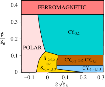
Figure 1: Phase diagram function of $g_{0}/g_{6}$ and $\tilde{p}/g_{6}$, where $\tilde{p}=2g_{S}\mu_{B}B/N\beta$.

Let us consider a magnetic field in the $z$-direction. Hence, the ground-state magnetization must be aligned with the external field, and $f_{+}=f_{-}=0$. Then, we obtain that $\sum_{ij}O_{ij}^{2}=77-12\gamma_{z}+3\gamma_{z}^{2}/2-f_{z}^{2}/2+|\eta|^{2}/2+2|\sigma|^{2}$, where $\gamma_{z}=\sum_{m}m^{2}|\psi_{m}|^{2}$, $\eta=\sum_{m=-3}^{1}\sqrt{[12-(m+2)(m+1)][12-m(m+1)]}\psi_{m+2}^{*}\psi_{m}$, and $\sigma=\sum_{m=-3}^{2}m\sqrt{[12-m(m+1)]}\psi_{m+1}^{*}\psi_{m}$. Removing spin-independent terms, the energy becomes $E=N\beta\epsilon/2$, with

$$\epsilon=\tilde{p}f_{z}+\tilde{c}_{1}f_{z}^{2}+\frac{4c_{2}}{7}|s_{-}|^{2}+c_{3}\left(\frac{3\gamma_{z}^{2}}{2}-12\gamma_{z}+\frac{|\eta|^{2}}{2}+2|\sigma|^{2}\right),$$ (7)

where $\tilde{p}=2p/N\beta$, and $\tilde{c}_{1}=c_{1}-c_{3}/2+\sqrt{16\pi/5}\Gamma_{0}c_{d}/\beta$. Since $c_{d}\ll c_{1}$, dipolar effects are not relevant for the equilibrium discussion. We will hence set $\Gamma_{0}=0$.

We have minimized Eq. (7) with respect to $\psi_{m}$, under the constraints $\sum_{m}|\psi_{m}|^{2}=1$ and $f_{+}=0$ footnote1 . Figs. 1 shows the corresponding phase diagram, which although in basic agreement with that worked out recently in Ref. Diener05 presents certain differences in its final form. For the phases discussed below $\sigma=0$ footnoteZ . For sufficiently negative $g_{0}$ the system is in a polar phase $P=({\bf c}\theta,0,0,0,0,0,{\bf s}\theta)$, with ${\bf c}\equiv\cos$, and ${\bf s}\equiv\sin$. This phase is characterized by $f_{z}\simeq-3\tilde{p}/\tilde{p}_{c}$ ($p_{c}\simeq 6\tilde{c}_{1}\simeq 0.36$), $4|s_{-}|^{2}=1-(\tilde{p}/\tilde{p}_{c})^{2}$, $\gamma_{z}=9$, and $|\eta|=0$. The polar phase extends up to $g_{0}/g_{6}=0.01$ for $p=0$. For sufficiently large $g_{0}$ and $\tilde{p}$, $CY_{-3,2}=({\bf c}\theta,0,0,0,0,{\bf s}\theta,0)$ occurs. This phase is cyclic ($s_{-}=0$) and it is characterized by $f_{z}=-3\tilde{p}/\tilde{p}_{c}$, $\gamma_{z}\simeq 6+3\tilde{p}/\tilde{p}_{c}$, and $|\eta|=0$. Both P and $CY_{-3,2}$ continuously transform at $\tilde{p}=\tilde{p}_{c}$ into a ferromagnetic phase $F=(1,0,0,0,0,0,0)$. For $0.04<\tilde{p}\leq 2\tilde{c}_{1}+9c_{3}$ $CY_{-3,2}$ becomes degenerated with the cyclic phase $CY_{-1,2}=(0,0,{\bf c}\theta,0,0,0,{\bf s}\theta,0)$. The latter state differs from $CY_{-3,2}$, since $\gamma_{z}=2-3\tilde{p}/\tilde{p}_{c}$. For sufficiently large $g_{0}$ and $\tilde{p}<0.04$, a cyclic phase ($CY_{-3,-1,1,3}$) of the form $(\psi_{-3},0,\psi_{-1},0,\psi_{1},0,\psi_{-3})$ occurs. Contrary to the other cyclic phases this phase is characterized by $|\eta|>0$ FootnoteBiaxial . Finally for a region around $g_{0}=0$ an additional phase with $|\eta|>0$, $|s_{-}|>0$ is found. In this phase two possible ground states are degenerated footnoteG , namely $S_{-2,0,2}=(0,\psi_{-2},0,\psi_{0},0,\psi_{+2},0)$, and $S_{-3,-1,1,3}$, which has a similar form as $CY_{-3,-1,1,3}$.

For a Cr-BEC in a spherical trap of frequency $\omega$ in the Thomas-Fermi regime, $\tilde{p}=\tilde{p}_{c}$ for a magnetic field (in mG) $B\simeq 1.25\left(N/10^{5}\right)^{2/5}\left(\omega/10^{3}\times 2\pi\right)^{6/5}$. Hence, most probably, magnetic shielding seems necessary for the observation of non-ferromagnetic ground-state phases. We would like to stress as well, that there are still uncertainties in the exact values of $a_{2,4,6}$. In this sense, we have checked for $a_{6}=98a_{B}$, $a_{4}=64a_{B}$, and $a_{2}=-27a_{B}$, that apart from a shift of $0.2$ towards larger values of $g_{0}/g_{6}$, the phase diagram remains qualitatively the same.

In the last part of this Letter, we consider the spinor dynamics within the MF approximation, but abandoning the SMA. The equations for the dynamics are obtained by deriving the MF Hamiltonian with respect to $\psi_{m}^{*}({\bf r})$:

$$i\hbar\frac{\partial}{\partial t}\psi_{m}({\bf r}) = \left[\frac{-\hbar^{2}\nabla^{2}}{2M}+U_{trap}+pm\right]\psi_{m}$$ (8)

$$+ N\left[c_{0}n+m(c_{1}f_{z}+c_{d}{\cal A}_{0})\right]\psi_{m}$$

$$+ \frac{N}{2}\left[c_{1}f_{-}+2c_{d}{\cal A}_{-}\right]S^{+}_{m,m-1}\psi_{m-1}$$

$$+ \frac{N}{2}\left[c_{1}f_{+}+2c_{d}{\cal A}_{+}\right]S^{-}_{m,m+1}\psi_{m+1}$$

$$+ (-1)^{m}\frac{2Nc_{2}}{7}s_{-}\psi_{-m}^{*}$$

$$+ Nc_{3}\sum_{n}\sum_{i,j}O_{ij}(S^{i}S^{j})_{mn}\psi_{n},$$

where ${\cal A}_{0}=\sqrt{6\pi/5}[\sqrt{8/3}\Gamma_{0,z}+\Gamma_{1,-}+\Gamma_{-1,+}]$, ${\cal A}_{\pm}=\sqrt{6\pi/5}[-\Gamma_{0,\pm}/\sqrt{6}\mp\Gamma_{\pm,z}+\Gamma_{\pm 2,\mp}]$, $\Gamma_{m,i}=\int d{\bf r}^{\prime}f_{i}({\bf r}^{\prime})Y_{2m}({\bf r}-{\bf r}^{\prime})/|{\bf r}-{\bf r}^{\prime}|^{3}$, and $S^{\pm}_{m,m\mp 1}=\sqrt{12-m(m\mp 1)}$. Note that all $\psi_{m}$, $n$, $f_{i}$, $O_{ij}$, and ${\cal A}_{i}$ have now a spatial dependence. We first consider $p=0$, and discuss on $p\neq 0$ below. There are two main features in the spinor dynamics in Cr-BEC which are absent (or negligible) in other spinor BECs. On one side the $c_{3}$ term allows for jumps in the spin manifold larger than one, and hence for a rapid dynamics from e.g. $m=0$ to $m=\pm 3$. On the other side, the dipolar terms induce a EH-like transfer of spin into CM angular momentum.

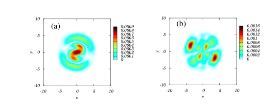
Figure 2: $|\psi_{m=-2}({\bf r})|^{2}$ at $\omega t=40$ (a) and $120$ (b) for $p=0$, $g_{0}=0$, $\omega_{z}=1$kHz, $N=10^{4}$ atoms, and $\psi(t=0)=\psi_{m=-3}$. The $x$ and $y$ axes are in $\sqrt{\hbar/m\omega}$ units.

We consider for simplicity a quasi-2D BEC, i.e. a strong confinement in the $z$-direction by a harmonic potential of frequency $\omega_{z}$. Hence $\psi_{m}({\bf r})=\phi_{0}(z)\psi_{m}({\bf\rho})$, where $\phi_{0}(z)=\exp[-z^{2}/2l_{z}^{2}]/\pi^{1/4}\sqrt{l_{z}}$, with $l_{z}=\sqrt{\hbar/m/\omega_{z}}$. We have then solved the 2D equations using Crank-Nicholson method, considering a harmonic confinement of frequency $\omega$ in the $xy$-plane. In 2D, $\Gamma_{\pm 1,z}=0$, but these terms vanish also in 3D due to symmetry, and hence the 2D physics is representative of the 3D one. The vanishing of $\Gamma_{\pm 1,z}$ is rather important, since if $\psi(t=0)=\psi_{m=\pm 3}$, $\Gamma_{\pm 1,z}$ is responsible for a fast dipolar relaxation (for $\omega t\sim 1$). Hence, a BEC with $\psi(t=0)=\psi_{\pm 3}$ does not present any significant fast spin dynamics. However significant spin relaxation appears in the long time scale, due to the $\Gamma_{2,-}({\bf r})$ terms. This is the case of Fig. 2, where we $\psi(t=0)=\psi_{m=-3}$ footnote2 .

One of the most striking effects related with spin relaxation is the transference of spin into CM angular momentum, which resembles the famous EH effect Einstein15 . The analysis of this effect motivated us to avoid the SMA in the study of the spinor dynamics. In Figs. 2 we show snapshots of the spatial distribution of the $m=-2$ component. Observe that the wavefunction clearly loose its polar symmetry, since spin is converted into orbital angular momentum. The spatial patterns become progressively more complicated in time.

The other special feature of Cr-BEC, namely the appearance of the $c_{3}$ term can have significant qualitative effects in the dynamics both for short and for long time scales. The evolution at long time scale may present interesting features, as large revivals, and it will be considered in future work. Here, we would like to focus on the short-time scales, where the $c_{3}$ term may produce fast transference from $\psi_{m=0}$ to the extremes $\psi_{m=\pm 3}$. The latter is illustrated in Fig. 3, where we consider $g_{0}=g_{6}$. The population is initially all in the $m=0$ footnote2 . Contrary to the case of $F=2$ in ⁸⁷Rb Schmaljohann04 , there is at short time scales a jump to the extremes (the population of $\pm m$ is the same due to symmetry since $p=0$). This large jump is absent if $c_{3}=0$, and depends on the value of $g_{0}$. In particular, if $g_{0}=0$ one obtains at short time scales a sequential population as for $F=2$ ⁸⁷Rb Schmaljohann04 .

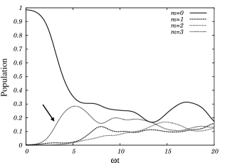
Figure 3: Population of $\psi_{0,1,2,3}$ versus $\omega t$ for $g_{0}=g_{6}$, $p=0$, and $\psi(0)=\psi_{0}$. Note the rapid growth of $m=\pm 3$ (arrow).

We finally comment on the dynamics if $p\neq 0$. In the case of $F=1$ or $F=2$ ⁸⁷Rb, the dynamics is independent of $p$ since the linear Zeeman effect may be gauged out by transforming $\psi_{m}\rightarrow\psi_{m}e^{ipmt/\hbar}$, due to the conservation of the total spin. In Cr-BEC the situation is very different, since the $\Gamma_{\pm 1,z}$ and $\Gamma_{\pm 2,\mp}$ do not conserve the total spin, and hence oscillate with the Larmor frequency $\omega_{L}=p/\hbar$ and $2\omega_{L}$, respectively. If $\omega_{L}\gg\omega$ one may perform rotating-wave approximation and eliminate these terms. Hence the coherent EH-like effect disappears for sufficiently large applied magnetic fields.

In conclusion, spin-3 Cr-BEC is predicted to show different types of spin phases depending on $a_{0}$ and the magnetic field. The spinor dynamics also presents novel features, as a fast transference between $\psi_{0}\rightarrow\psi_{\pm 3}$, and the Einstein-de Haas-like transformation of spin into rotation of the different components due to the dipole interaction.

We would like to thank M. Fattori for enlightening discussions, and the German Science Foundation (DFG) (SPP1116 and SFB/TR 21) for support. We thank H. Mäkelä and K.-A. Suominen for pointing us a mistake in previous calculations, and T.-L. Ho for enlightening e-mail exchanges. During the elaboration of the final version of this paper, the EH-effect has been also discussed in Ref. Kawaguchi05 .

References

(1) T.-L. Ho, Phys. Rev. Lett. 81, 742 (1998).
(2) T. Ohmi and K. Machida,
J. Phys. Soc. Jpn. 67, 1822 (1998).
(3) C. K. Law, H. Pu, and N. P. Bigelow, Phys. Rev. Lett.
81, 5257 (1998); H. Pu et al., Phys. Rev. A 60, 1463 (1999).
(4) M. Koashi and M. Ueda, Phys. Rev. Lett. 84,
1066 (2000).
(5) C. V. Ciobanu, S.-K. Yip, and T.-L. Ho, Phys. Rev. A,
61, 033607 (2000).
(6) M. Koashi and M. Ueda, Phys. Rev. Lett. 84,
1066 (2000); M. Ueda and M. Koashi, Phys. Rev. A 65, 063602 (2002).
(7) H. Pu, W. Zhang, and P. Meystre, Phys. Rev. Lett.
87, 140405 (2001).
(8) S. Yi, L. You, and H. Pu, Phys. Rev. Lett. 93,
040403 (2004).
(9) T.-L. Ho and S. K. Yip, Phys. Rev. Lett. 84,
4031 (2000); Ö. E. Müstercaplıoğlu et al, Phys. Rev. A 68,
063616 (2003).
(10) D. S. Hall et al., Phys. Rev. Lett. 81,
1539 (1998).
(11) J. Stenger et al., Nature 396, 345 (1998).
(12) M. D. Barret, J. A. Sauer, and M. S. Chapman,
Phys. Rev. Lett. 87, 010404 (2001).
(13) H. Schmaljohann et al., Phys. Rev. Lett.
92, 040402 (2004).
(14) M.-S. Chang et al., Phys. Rev. Lett.
92, 140403 (2004); W. Zhang et al., Phys. Rev. A 72,
013602 (2005).
(15)
T. Kuwamoto et al., Phys. Rev. A 69, 063604 (2004).
(16) M. H. Wheeler et al., Phys. Rev. Lett. 93, 170402 (2004).
(17) J. M. Higbie et al. Phys. Rev. Lett. 95,
050401 (2005).
(18) A. Widera et al., cond-mat/0505492.
(19) N. N. Klausen, J. L. Bohn, and C. H. Green, Phys. Rev. A
64, 053602 (2001).
(20) A. Griesmaier et al., Phys. Rev. Lett. 94,
160401 (2005).
(21) S. Yi and L. You, Phys. Rev. A 61, 041604 (2000);
K. Góral, K. Rza̧żewski, and T. Pfau, Phys. Rev. A
61, 10501601(R) (2000); L. Santos et al.,
Phys. Rev. Lett. 85, 1791 (2000);
L. Santos, G. V. Shlyapnikov, and M. Lewenstein,
Phys. Rev. Lett. 90, 250401 (2003).
(22) J. Stuhler et al. Phys. Rev. Lett. 95, 150406 (2005).
(23) R. Diener, and T.-L. Ho, cond-mat/0511751.
(24) A. Einstein and W. J. de Haas, Verhandl. Deut. Physik Ges. 17, 152 (1915).
(25) J. Werner et al., Phys. Rev. Lett. 94, 183201
(2005).
(26) For every and
we performed up to different runs of a simulated annealing
method to avoid the numerous local minima.
(27) We also found numerically states (similar to the Z states of Ref. Diener05 )
with tiny , which are however very slight variations of neighboring phases,
with which they are in practice degenerated.
(28) leads to the interesting possibility of biaxial nematics, as recently
pointed out for the first time in Ref. Diener05 .
(29) These phases are degenerated for any practical purposes, with relative energy differences .
(30) A small seed in the other components triggers the mean-field evolution.
(31) H. Saito, and M. Ueda, cond-mat/0506520.
(32) Y. Kawaguchi, H. Saito, and M. Ueda, cond-mat/0511052.