Thermoelectric transport near the pair breaking quantum phase transition out of a $d$-wave superconductor

Abstract

We study electric, thermal, and thermoelectric conductivities in the vicinity of a $z=2$ superconductor-diffusive metal transition in two dimensions, both in the high and low frequency limits. We find violation of the Wiedemann-Franz law and a dc thermoelectric conductivity $\alpha$ that does not vanish at low temperatures, in contrast to Fermi liquids. We introduce a Langevin equation formalism to study critical dynamics over a broad region surrounding the quantum critical point.

I Introduction

Transport of heat and charge provide a useful probe of strongly correlated electronic systems. For example, a violation of the Wiedemann-Franz law at low temperatures signals non-Fermi liquid physics. One possible origin of such a violation is proximity to a quantum critical point (QCP), where the presence of low energy critical modes leads to novel phenomena. There has been much theoretical and experimental attention directed towards electrical transport at QCP’s, in the context of the superconductor-insulator transition in amorphous films, and the Quantum Hall transitions (see Sachdev (1999); Sondhi et al. (1997) for reviews). Recently, experimental investigations of thermal and thermoelectric properties at quantum phase transitions have been pursued with very interesting results. These include measurements of thermal conductivity in highly underdoped cuprate systems near critical doping Sutherland et al. (2005); Proust et al. , and of thermoelectric transport (Nernst and Seebeck coefficients) near a heavy fermion QCP Bel et al. (2004). However, there has been relatively little theoretical work on thermal and thermoelectric transport at QCP’s. In this paper we calculate the nontrivial electric, thermal, and thermoelectric conductivities at a $z=2$, $d=2$ quantum critical point for the transition from an unconventional (non $s$-wave) superconductor to a diffusive metal in 2 dimensions.

In an applied electric field $E$ and temperature gradient $\nabla T$, the electric ($\sigma$), thermal ($\kappa$), and thermoelectric ($\alpha$) conductivities are defined by,

$$\left(\begin{array}[]{c}j\\ j_{Q}\end{array}\right)=\left(\begin{array}[]{c c}\sigma&\alpha\\ \alpha T&\tilde{\kappa}\end{array}\right)\left(\begin{array}[]{c}E\\ -\nabla T\end{array}\right).$$ (7)

where $j$ and $j_{Q}$ are the electrical and heat currents, respectively. Thermal conductivity measurements are always carried in open circuit ($j=0$) boundary conditions, so that $\kappa=\tilde{\kappa}-\alpha^{2}T/\sigma$. The difference between $\kappa$ and $\tilde{\kappa}$ is negligible in metals, but this need not be the case in systems with strong particle-hole symmetry breaking, as considered here. Our results are shown in Table 1. We find that, while the dc thermal conductivity is metallic, the dc electric conductivity diverges as $T\to 0$. Hence, there is a strong violation of Wiedemann-Franz law (WF) in the bosonic sector, with an apparent excess of charge carriers. The total conductivities are sums of fermionic and bosonic parts, $\sigma=\sigma_{f}+\sigma_{\Phi}$ (and similarly for $\alpha$, $\kappa$). Thus, the magnitude of the expected WF violation is difficult to estimate. Another striking effect is that $\alpha_{\Phi}$ has a very weak $T$ dependence at low temperatures ($\sim\ln\ln T$), unlike $\alpha_{f}$, which vanishes linearly with $T$. Hence, experimental measurement of the anomalous thermoelectric conductivity would give direct information regarding critical transport properties, as well as yielding the dimensionless “thermoelectric figure of merit” $ZT={\alpha^{2}T\over\sigma\kappa}$, a measure of the strength of particle-hole breaking.

	$T=0$	$\Omega=0$
$\sigma$	const	$\frac{(2e)^{2}}{h}\frac{b}{8\pi^{2}\eta}\ln\frac{\Lambda}{T}$
$\alpha$	$\sim i\frac{\Omega}{T}$	$\frac{2ek_{B}}{h}\frac{1}{8\pi^{2}\eta}\ln{\ln\frac{\Lambda}{T}}$
$\tilde{\kappa}/T$	$\sim\frac{\Omega^{2}}{T^{2}}$	const

Table 1: Asymptotic low $T$ behavior of transport coefficients along the line $s=s_{c}$ in the zero temperature ($\Omega/T\to\infty$) and dc ($\Omega/T\to 0$) limits. The prefactor of $\sigma(\Omega=0)$ is given in an extreme low $T$ limit $b=[{\tan^{-1}({1}/{\eta})+{4\eta}/({1+\eta^{2}})}]/{2\ln\ln(\Lambda/T)}$. Improved values for the $\Omega=0$ results, valid for a broader $T$ range appear below Eq. (28). Explicit expressions for $\sigma(T=0)$ and $\tilde{\kappa/T}(\Omega=0)$ are given in Eqs. (13) and (14).

A QCP with either Lorentz or Galilean invariance will have infinite thermal conductivity, because a “boosted” thermal distribution will never decay; the same logic applies to electric conductivity if there is only one sign of charge carrier. We find below that a finite $\eta$ at the $z=2$ QCP regularizes the thermal conductivity. It is also crucial that the $z=2$ theory breaks particle-hole symmetry so that the thermoelectric coefficient can be nonzero; the $z=2$ theory is thus the simplest critical theory for which all the transport coefficients in (7) are finite.

II Model and currents

Our starting point is an electron model with a pairing interaction favoring unconventional superconductivity, and a disorder potential whose main effect is to render electrons diffusive. Then, introducing a Hubbard-Stratanovich field $\Phi$ in the Cooper channel and integrating out fermions yields a Ginsburg-Landau action for $\Phi$,Herbut (2000)

$$S[\Phi] = \int_{0}^{\beta}d\tau\int d^{2}r\left[\Phi^{*}\left(\partial_{\tau}+\eta|\partial_{\tau}|-\frac{1}{2m}\nabla^{2}+s\right)\Phi\right.$$ (8)

$$\left.+\frac{V}{2}|\Phi|^{4}\right],$$

where the dissipative term $|\partial_{\tau}|$, shorthand for the Matsubara expression $|\omega_{n}|$, arises from the decay of Cooper pairs into gapless fermions. Note that, for unconventional superconductors, disorder is pair-breaking. This insures that the critical theory (8) is localHerbut (2000). Naive power counting of model (8) yields dynamical critical exponent $z=2$. Although disorder dominates extremely close to the transition, one can choose microscopic parameters such that eq. (8) describes a large crossover region near the QCPHerbut (2000). For instance, for a clean sample with an elastic mean free path of 100 nm, Model (8) is valid provided $T$ is larger than a few millikelvinthermoelectricLargeN . This paper focuses on transport in this region. Equation (8) also applies to the onset of antiferromagnetic order in an itinerant electron systemMillis (1993), with $\Phi$ an O(3) order parameter. Many of our results apply to this QCP as well (eg. thermal conductivity) but the field $\Phi$ carries spin, and not charge.

The electric and heat currents $j=\frac{\partial S}{\partial A_{e}}$ and $j_{Q}=\frac{\partial S}{\partial A_{T}}$ are obtained by making the action (8) gauge-covariant through the substitution $\nabla\to{\cal D}\equiv\nabla-ieA_{e}-iA_{T}(i\partial_{t})$ (see Ref. Moreno and Coleman ),

$$j = \frac{ie}{m}\left(\Phi^{\dagger}{\cal D}\Phi-({\cal D}\Phi)^{\dagger}\Phi\right)$$

$$j_{Q} = \frac{1}{2m}\left((\partial_{t}-is)\Phi^{\dagger}{\cal D}\Phi+({\cal D}\Phi)^{\dagger}(\partial_{t}+is)\Phi\right)$$

We compute conductivities from Kubo formulas involving the dynamical correlations of these currents.

III Order of $T\to 0$ and $\Omega\to 0$ limits

Conductivities near the $2d$ QCP depend on ratios of small energy scales (and possibly a UV cutoff scale $\Lambda$), and on the dimensionless parameters $mV$ and $\eta$,

$$G_{\gamma}(\Omega)=g_{\gamma}\left(\frac{|s-s_{c}|^{\nu z}}{T},\frac{\Omega}{T},\frac{\Lambda}{T},mV,\eta\right).$$ (9)

Here, $G_{0}\equiv\sigma$, $G_{1}\equiv\alpha$, and $G_{2}\equiv\tilde{\kappa}/T$, $\Omega$ is the frequency of the external field, and $\nu z=1$ for the $d=2$, $z=2$ model in question. At the QCP, $s=s_{c}$, $G_{\gamma}$ depend on the order of the limits $\Omega\to 0$ and $T\to 0$Damle and Sachdev (1997). Sending $\Omega\to 0$ first yields the dc conductivities, which are more readily accessible to experiment, but are typically more difficult to compute than their $T=0$ analogs.

For a $d=2$, $z=2$ theory, the quartic interaction $V$ is dangerously irrelevant. Thus, at the $T=0$ QCP, the correct dynamics is obtained from the limit $V\to 0^{+}$. We first consider this non-interacting case. Note that, even without interactions, finite transport is plausible, due to dissipation in action (8). Indeed, $\sigma$ is metallic in the zero temperature limitHerbut (2000), as shown in the middle column of Table 1. On the other hand, to compute dc conductivities, we shall consider finite temperatures, for which interactions give important logarithmic corrections.

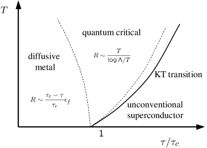
Figure 1: Phase diagram in the vicinity of the QCP as a function of disorder, parameterized by the lifetime $\tau$ of electrons in the diffusive metal. At finite $T$, interactions shift the transition line to the right, so that the diffusive metal phase lies above the QCP. The crossover into the quantum critical regime occurs when $R\approx T$.

IV Non-interacting case

The conductivities are obtained from Kubo formulas, $G_{\gamma}(\Omega)=\frac{(2e)^{2-\gamma}k_{B}^{\gamma}}{i\Omega T^{\gamma}}\Pi_{\gamma}(\Omega+i\delta)$. For $V=0$, $\Pi_{\gamma}$ is given by a single-loop integral,

$$\Pi_{\gamma}(i\Omega_{n}) = \frac{i^{\gamma}}{\beta}\sum_{\omega_{n}}\int{\frac{d^{2}k}{(2\pi)^{2}}}\frac{k_{x}^{2}}{m^{2}}\left\{-\omega_{n}^{\gamma}{\cal{G}}(k,\omega_{n})^{2}\right.$$

$$+ \left.(\omega_{n}+\Omega_{n}/2)^{\gamma}{\cal{G}}(k,\omega_{n}){\cal{G}}(k,\omega_{n}+\Omega_{n})\right\},$$

where ${\cal{G}}$ is the Matsubara Green’s functions, ${\cal{G}}(k,\omega_{n})=\left(i\omega_{n}-\eta|\omega_{n}|-\epsilon_{k}-s\right)^{-1},$ where $\epsilon_{k}=k^{2}/2m$. Rewriting this in terms of the spectral function, ${\cal{G}}(k,\omega_{n})=\int\frac{d\omega^{\prime}}{2\pi}\frac{{\cal{A}}(k,\omega^{\prime})}{i\omega_{n}-\omega^{\prime}}$, ${\cal{A}}(k,\omega)=\frac{2\eta\omega}{(\omega-\epsilon_{k}-s)^{2}+\eta^{2}\omega^{2}}$, we obtain,

$$\Pi_{\gamma}(i\Omega_{n}) = \frac{1}{\beta}\sum_{\omega_{n}}\int_{\omega_{1},\omega_{2},{\bf k}}\left(\frac{\omega_{1}+\omega_{2}}{2}\right)^{\gamma}{\cal{A}}(k,\omega_{1}){\cal{A}}(k,\omega_{2})$$ (11)

$$\frac{k_{x}^{2}}{m^{2}}\left\{\frac{1}{(i\omega_{n}-\omega_{1})(i(\omega_{n}+\Omega_{n})-\omega_{2})}\right.$$

$$\left.-\frac{1}{(i\omega_{n}-\omega_{1})(i\omega_{n}-\omega_{2})}\right\},$$

In (11) we have made the substitution $i\omega_{n}\to(\omega_{1}+\omega_{2})/2$. This accounts for the fact that the time derivative in $j_{Q}$ does not commute with the time-ordering symbol, and is necessary to obtain the correct thermal conductivity Ambegaokar and Griffin (1964). Performing the $\omega_{n}$ sum and using the identity, $f^{0}(\omega+i\Omega_{n})=f^{0}(\omega)$, before analytically continuing to real frequencies, $i\Omega_{n}\to\Omega+i\delta$, we find

$${\rm Im} \Pi_{\gamma}(\Omega+i\delta)=\frac{1}{2}\int_{\omega_{2},{\bf k}}\frac{k_{x}^{2}}{m^{2}}\left(\omega_{2}-\frac{\Omega}{2}\right)^{\gamma}\times$$

$${\cal{A}}(k,\omega_{2}-\Omega){\cal{A}}(k,\omega_{2})\left(f^{0}(\omega_{2}-\Omega)-f^{0}(\omega_{2})\right),$$

where $f^{0}(\omega)=(\exp\left(\beta\omega\right)-1)^{-1}$ is the Bose occupation factor. The integrals are UV finite, and hence the dependence on the cutoff $\Lambda$ drops out,

$$G_{\gamma}^{\rm scaling}(\Omega)=g^{\rm scaling}_{\gamma}\left(\frac{|s-s_{c}|^{\nu z}}{T},\frac{\Omega}{T},\eta\right).$$

Expression (IV) can readily be evaluated for generic $\Omega/T$.

IV.1 Zero temperature ($\Omega/T\to\infty$) limit

The results in the zero temperature limit at the QCP ($s=s_{c}=0$) are summarized in the middle column of Table 1. While $\sigma$ is metallic, $\alpha$ and $\tilde{\kappa}/T$ are divergent (note that $\alpha$ is purely reactive). The electric conductivity depends on the dissipation $\eta$,

$$\sigma\left(\frac{\Omega}{T}\to\infty\right) = \frac{(2e)^{2}/h}{4\pi\eta^{2}}\left\{[2\eta+\pi(1+\eta^{2})]\arctan\eta\right.$$ (13)

$$\left.-\pi\eta-\eta^{2}-(1+\eta^{2})\arctan^{2}\eta\right\},$$

since $\eta$ is marginal.

IV.2 DC ($\Omega/T\to 0$) limit

On the other hand, the dc transport properties at $V=0$ are drastically different. Whereas $\sigma=\frac{(2e)^{2}}{h}\frac{T}{4|\Omega|}$ and $\alpha=\frac{2ek_{B}}{h}\frac{1}{8\pi^{2}\eta}\ln\frac{T}{|\Omega|}$ are divergent, $\frac{\tilde{\kappa}}{T}$ is metallic,

$$\frac{\tilde{\kappa}}{T}\left(\frac{\Omega}{T}\to 0\right)=\frac{k_{B}^{2}}{h}\left(\frac{\eta+\arctan(1/\eta)}{12\pi\eta}\right)$$ (14)

In order to elucidate the dc results, we employ a simple Boltzmann equation approach, which is exact for weak dissipation $\eta\to 0$. The dissipating term in the action (8) can be interpreted as the self-energy of bosons due to their interactions with the fermion bath,

$$\Sigma(i\omega_{n})=\eta|\omega_{n}|.$$

This is purely imaginary for real frequencies ($|z|=z\,{\rm sign}({\rm Re}\,z)$). Hence, while the energy of a quasi particle is not renormalized, quasi particles are given a finite lifetime,

$$\frac{1}{\tau_{k}} = i\left[\Sigma(\omega+i\delta)-\Sigma(\omega-i\delta)\right]_{\omega=\epsilon_{k}}=2\eta\epsilon_{k}.$$ (15)

This is the boson lifetime, at bubble level, in the fermion model. Here we neglect corrections to the transport lifetime from higher order diagrams.

The Boltzmann equation for the occupation function $f({\bf k},{\bf r},t)$ in the scattering lifetime approximation yields

$$\partial_{t}f+{\bf v}\cdot\nabla_{\bf r}f+\dot{{\bf k}}\cdot\nabla_{\bf k}f=-\frac{1}{\tau_{\bf k}}(f-f^{0}).$$ (16)

The electric and energy currents are expressed in terms of $f$,

$$j^{a}({\bf r},t) = \int{\frac{d^{2}k}{(2\pi)^{2}}}\,(2e)v_{\bf k}^{a}f({\bf k},{\bf r},t)$$ (17)

$$j^{a}_{Q}({\bf r},t) = \int{\frac{d^{2}k}{(2\pi)^{2}}}\,(\epsilon_{\bf k}-s)v_{\bf k}^{a}f({\bf k},{\bf r},t).$$ (18)

The conductivities are then

$$G_{\gamma}=\frac{(2e)^{2-\gamma}k_{B}^{\gamma}}{T^{\gamma}\hbar}\int{\frac{d^{2}k}{(2\pi)^{2}}}\,\frac{\tau_{\bf k}}{1-i\Omega\tau_{\bf k}}\frac{\epsilon_{k}^{1+\gamma}}{m}\left(-\frac{\partial f^{0}}{\partial\epsilon_{\bf k}}\right).$$ (19)

For $\eta\to 0$, this gives perfect agreement with the previous results for $G_{\gamma}$ in the dc limit. Here, we see that the reason for the divergences in $\sigma$ and $\alpha$ is that low energy quasiparticles have arbitrarily large lifetimes $\tau_{\bf k}$. On the other hand, these very long-lived quasiparticles, having low energies, contribute little to the energy current. Hence $\tilde{\kappa}/T$ is finite.

V Interacting case

For $T>0$, the dangerously irrelevant interaction $V$ must be taken into account. The most important effect of interactions is to shift the phase transition, such that the QCP is approached at finite temperatures from the diffusive metal phase, as shown in Fig. 1. This is captured by a renormalized mass $R$, discussed below, which is positive above the transition. $R$ acts as an effective gap for low energy quasiparticles, thus rendering all dc transport coefficients finite. The situation is in contrast with Ref. Damle and Sachdev (1997), where interactions regularize transport by introducing quasiparticle scattering. Here, the leading low $T$ dc conductivities are obtained from a Hartree-Fock (HF) analysis, where the only effect of interactions is to shift the quasiparticle mass $R$. The HF results are shown in the last column of Table 1. These results are valid for extremely low temperatures, such that $\ln\ln\Lambda/T\gg 1$. To study transport on a much broader region surrounding the QCP, we introduce a classical treatment of the order parameter which, when supplemented by Langevin dynamics, will be shown to capture the correct quantum critical transport behavior over the region where the much weaker condition, $\ln\Lambda/T\gg 1$, is satisfied.

V.1 Classical action for order parameter

With interactions, the critical point is shifted away from $s_{c}=0$. To linear order in $V$,

$$s_{c}=2V\int_{\omega,k}\frac{1}{i\omega_{n}-\eta|\omega_{n}|-\epsilon_{k}}$$

In the vicinity of the QCP, we renormalize $V$ by a one loop RG equation, up to the scale where the system either develops a gap, or when the rescaled temperature reaches an upper frequency cutoff $\Lambda_{\omega}$Fisher and Hohenberg (1987); Millis (1993),

$$V_{R}\approx\frac{2\pi^{2}}{m\left(\tan^{-1}\frac{1}{\eta}+\frac{4\eta}{1+\eta^{2}}\right)}\frac{1}{\ln\frac{\Lambda_{\omega}}{{\rm Max}(T,|s-s_{c}|)}}$$

The static properties of the finite $T$ model can be studied by integrating out all non-zero Matsubara frequency modes. After rescaling, $\Phi=\sqrt{2mT}\psi$, ${\bf r}={\bf x}/\sqrt{2m},$ the $\omega_{n}=0$ mode has the following classical action,

$$S_{c}=\int d^{2}x\left[|\nabla_{x}\psi|^{2}+\tilde{R}|\psi|^{2}+\frac{U}{2}|\psi|^{4}\right]$$

where $U=2mTV_{R}$. This theory is super-renormalizable, and is rendered UV finite by introducing a renormalized mass $R$,

$$\tilde{R}=R-2U\int_{0}^{\Lambda}{\frac{d^{2}k}{(2\pi)^{2}}}\frac{1}{k^{2}+R}.$$ (20)

$R$ has a universal expression in terms of $s-s_{c}$, reflecting the contribution of the $\omega_{n}\neq 0$ modes

$$R = (s-s_{c})+\frac{U}{2\pi T}\int_{0}^{\infty}dy\left[\frac{T}{y+R}-\frac{T}{y+s-s_{c}}\right.$$ (21)

$$\left.+\int_{0}^{\infty}\frac{d\Omega}{\pi}\frac{\eta\Omega}{e^{\Omega/T}-1}\left(\frac{1}{(\Omega-y-(s-s_{c}))^{2}+\eta^{2}\Omega^{2}}\right.\right.$$

$$+\left.\left.\frac{1}{(\Omega+y+s-s_{c})^{2}+\eta^{2}\Omega^{2}}\right)\right]$$

$$= s-s_{c}+\frac{U}{2\pi}\left\{\ln\frac{T}{R}+F(s-s_{c},\eta)\right\},$$

where $F(s-s_{c},\eta)\to\ln\sqrt{1+\eta^{2}}$ as $s\to s_{c}$. Solving this self-consistent equation at $s=s_{c}$ yields,

$$R\sim\frac{T}{\ln(\Lambda_{\omega}/T)}$$ (22)

up to a prefactor of order $\ln\ln(\Lambda_{\omega}/T)$. Note that, for $T>0$, $R$ is always positive, even for arbitrarily negative values of $s-s_{c}$. This is due to the absence of long-range order (LRO) in $2d$ at finite $T$. For an O(2) order parameter, however, quasi LRO is established at a $T>0$ Kosterlitz-Thouless transition.

A description in terms of a classical action dunkel is appropriate whenever $\log\Lambda_{\omega}/T\gg 1$. In this limit, $U\ll T$, so that modes with $\omega_{n}\neq 0$ are significantly gapped.

V.2 Dynamics of order parameter

We approximate the low frequency dynamics of the classical order parameter by a Langevin equation (model A dynamics of Ref. Hohenberg and Halperin (1977)),

$$\frac{\partial\psi}{\partial t} = -(i+\eta)\frac{\delta S_{c}}{\delta\psi^{*}}+f_{\eta}$$ (23)

$$\langle f_{\eta}^{*}(x,t)f_{\eta}(x^{\prime},t^{\prime})\rangle = 2\eta\delta(x-x^{\prime})\delta(t-t^{\prime})$$

Equal time correlators computed with these dynamics are equal to those of the classical action $S_{c}$, as necessary. The appearance of the “bare” value of $\eta$ in eq. (23) is due to the fact that dispersion in the quantum action is non-local in time and therefore is not renormalized.

Consider the HF approximation, in which (23) becomes a linear equation with mass $R$. Solving for $\sigma$,

$${\rm Re}\,\sigma(\Omega) = \frac{(2e)^{2}}{h}\frac{T}{2\pi\Omega}\tan^{-1}\frac{\Omega}{4\eta R}$$ (26)

$$\to \frac{(2e)^{2}}{h}\left\{\begin{array}[]{c l}\frac{T}{4|\Omega|}&{\rm for}\,R=0\\ \frac{T}{8\pi\eta R}&{\rm for}R\neq 0,\,\Omega\to 0\end{array}\right.$$

For $R=0$, this reproduces the non-interacting result, as expected. On the other hand, for $R\neq 0$, we obtain a finite dc conductivity,

$$\sigma\sim\ln\frac{\Lambda_{\omega}}{T}$$ (27)

We note that Eq. (27) disagrees with Ref. Dalidovich and Phillips (2001), which predicts $\sigma\sim\ln\ln(\Lambda_{\omega}/T)$. This is due to an erroneous computation of $T^{*}$ in Eq. (12) of that reference.

Naive use of Eq. (23) yields divergent values of $\alpha$ and $\tilde{\kappa}/T$. This is not surprising: the Langevin equation assumes classical modes, whose occupation factors satisfy equipartition, $f_{\rm eq}(\omega)=T/\omega$. However, inspection of the Boltzmann approach, eq. (19), shows that for such distribution, $\alpha$ and $\tilde{\kappa}/T$ have UV catastrophes. In this sense, the Langevin equation does not capture the correct dynamics of high energy quantum modes. However, high energy modes are very weakly perturbed by the quartic interaction. Thus, the correct result is given by the Boltzmann equation with a full Bose distribution, as in Eq. (19), but with a chemical potential set by $R$. Equivalently, this corresponds to evaluating the one-loop quantum expression (11) with chemical potential $R$. This yields the last column of Table 1.

The HF results can be obtained independently from an exact solution of the quantum model (8) in the large $N$ limitthermoelectricLargeN , where $N$ is the number of components of the order parameter ($N=2$ for superconductivity). This is an important check that the Langevin equation (23) captures the correct universal dynamics. We see from Eq. (21) that, for $s=s_{c}$ and at low $T,$

$$\frac{U}{R}\propto\frac{1}{\ln T/R}\sim\frac{1}{\ln\ln\Lambda_{\omega}/T}$$

which justifies HF provided that $\ln\ln(\Lambda_{\omega}/T)$ is a large number. More generally, to go beyond HF, we must consider higher order corrections in $U$. From the Kubo formula and the fluctuation-dissipation theorem, we deduce that the dc electric conductivity obeys

$$\sigma=\frac{(2e)^{2}}{h}\frac{T}{8\pi\eta R}\Phi_{\sigma}\left(\frac{U}{R},\eta\right),$$ (28)

for some scaling function $\Phi_{\sigma}$ satisfying $\Phi_{\sigma}(0,\eta)=1$. A similar analysis applies to $\alpha$ and $\tilde{\kappa}/T$, with the important difference that substractions are necessary to cancel leading UV divergences, as discussed above. When working with the renormalized $R$, the only UV divergence comes from the diagrams already computed. Thus,

$$\alpha=\alpha_{\rm quantum,1\,loop}+\frac{2e}{2}\Phi_{\alpha}\left(\frac{U}{R},\eta\right),$$

$$\frac{\tilde{\kappa}}{T}=\frac{\tilde{\kappa}_{\rm quantum,1\,loop}}{T}+\frac{R}{2T}\Phi_{\kappa}\left(\frac{U}{R},\eta\right),$$

where the small $R$ limit of the (quantum, 1 loop) results is $\frac{2ek_{B}}{8\pi^{2}\eta h}\ln\frac{T}{R}$ for $\alpha$, and Eq. (14) for $\tilde{\kappa}/T$. The functions $\Phi_{\gamma}$ can be evaluated numerically by introducing a lattice,

$$S_{cL}=\sum_{\langle ij\rangle}|\psi_{i}-\psi_{j}|^{2}+\sum_{i}\left[\tilde{R}_{L}a^{2}|\psi_{i}|^{2}+\frac{Ua^{2}}{2}|\psi_{i}|^{4}\right]$$

and requiring that the renormalized $R$ be the same in the lattice and continuum theories,

$$\tilde{R}_{L}=R-2U\int_{-\pi}^{\pi}\frac{dk_{x}}{2\pi}\int_{-\pi}^{\pi}\frac{dk_{y}}{2\pi}\frac{1}{4-2\cos k_{x}-2\cos k_{y}+Ra^{2}}.$$

Fig. 2 shows the scaling function $\Phi_{\sigma}(U/R,\eta=1).$ This, combined with Eqs. (21) and (28), gives the electric conductivity for the entire quantum critical regime. We stress that these results rely only on the condition $\log\Lambda/T\gg 1$. This use of Langevin dynamics to obtain full scaling functions for transport quantities at a QCP should be applicable at many other transitions. Here, we have used them to find WF violation and an anomalous thermoelectric conductivity at a transition of experimental interest.

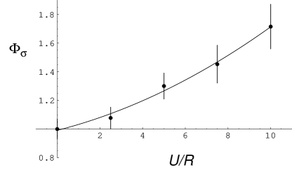
Figure 2: Estimated scaling function $\Phi_{\sigma}(U/R,\eta=1)$ from numerical integration of the Langevin equation (23). Convergence for static quantities of the Langevin algorithm was tested by comparison with results from a Wolff cluster algorithm. Each data point represents at least $2\times 10^{7}$ time steps on a lattice of spacing $a=0.1$ and linear size $L=64$, which for static quantities with $\eta=0$ is known to approximate well the continuum limit $a\rightarrow 0$. Results were normalized by the $U/R=0$ result and fit by a quadratic polynomial (solid line).

VI Conclusions

VII Acknowledgments

We benefited from useful discussions with B. Binz, A. Paramekanti, T. Senthil, and members of the 2005 Aspen Center for Physics Workshop on Competing Orders, where part of this work was completed. This work was supported by NSF grants DMR-0238760 (J.M.) and DMR-0537077 (S.S.), the Hellman Fund (J.M.), and the LDRD program of LBNL under DOE grant DE-AC02-05CH11231 (D.P. and A.V.).

References

- Sachdev (1999) S. Sachdev, Quantum Phase Transitions (Cambridge University Press, 1999).
- Sondhi et al. (1997) S. L. Sondhi et al., Rev. Mod. Phys. 69, 315 (1997).
- Sutherland et al. (2005) M. Sutherland et al., Phys. Rev. Lett. 94, 147004 (2005).
- (4) C. Proust et al., cond-mat/050551.
- Bel et al. (2004) R. Bel et al., Phys. Rev. Lett. 92, 217002 (2004).
- Herbut (2000) I. F. Herbut, Phys. Rev. Lett. 85, 1532 (2000).
- Millis (1993) A. J. Millis, Phys. Rev. B 48, 7183 (1993).
- Damle and Sachdev (1997) K. Damle and S. Sachdev, Phys. Rev. B 56, 8714 (1997).
- (9) J. Moreno and P. Coleman, cond-mat/9603079.
- Ambegaokar and Griffin (1964) V. Ambegaokar and A. Griffin, Phys. Rev. 137, A1151 (1964).
- Fisher and Hohenberg (1987) D. S. Fisher and P. C. Hohenberg, Phys. Rev. B 37, 4936 (1987).
- (12) S. Sachdev and E. R. Dunkel, Phys. Rev. B 73, 085116 (2006).
- Hohenberg and Halperin (1977) P. C. Hohenberg and B. I. Halperin, Rev. Mod. Phys. 49, 435 (1977).
- Dalidovich and Phillips (2001) D. Dalidovich and P. Phillips, Phys. Rev. B 63, 224503 (2001).
- (15) D. Podolsky, A. Vishwanath, J. E. Moore, and S. Sachdev (to appear).