Magnetic field effects and renormalization of the long-range Coulomb interaction in Carbon Nanotubes

Abstract

We develop two theoretical approaches for dealing with the low-energy effects of the repulsive interaction in one-dimensional electron systems. Renormalization Group methods allow us to study the low-energy behavior of the unscreened interaction between currents of well-defined chirality in a strictly one-dimensional electron system. A dimensional regularization approach is useful, when dealing with the low-energy effects of the long-range Coulomb interaction. This method allows us to avoid the infrared singularities arising from the long-range Coulomb interaction at $D=1$. We can also compare these approaches with the Luttinger model, in order to analyze the effects of the short range term in the interaction.

Thanks to these methods, we are able to discuss the effects of a strong magnetic field $B$ in quasi one-dimensional electron systems, by focusing our attention on Carbon Nanotubes. Our results imply a variation with $B$ in the value of the critical exponent $\alpha$ for the tunneling density of states, which is in fair agreement with that observed in a recent transport experiment involving carbon nanotubes. The dimensional regularization allows us to predict the disappearance of the Luttinger liquid, when the magnetic field increases, with the formation of a chiral liquid with $\alpha=0$.

I Introduction

In the last 20 years progresses in semiconductor device fabrication and carbon technology allowed for the construction of several new devices at the nanometric scale and many novel transport phenomena have been revealed in mesoscopic low-dimensional structures. The limits of further miniaturization (predicted by Moore’s law) have increased the research toward the development of electronics at the nanoscale and new efforts of scientists have been stimulated by the progress in carbon and semiconductor technology, aimed at building a nanoelectronics 1n ; 2n . One-dimensional (1D) nanodevices, such as carbon nanotubes (CNs) and semiconductor Quantum Wires (QWs), are the building blocks of this new kind of electronicsnoiras , and recent experiments have revealed that they are also excellent systems for the investigation of electronic transport in one dimension (for other low dimensional semiconductor devices, such as Quantum Dots, see e.g.noidot ).

Semiconductor QWs are quasi 1D devices (having a width smaller than $1000\AA$thor and a length of some microns) made from a two-dimensional electron gas (2DEG) created in heterostructures between different thin semiconducting layers (typically $GaAs:AlGaAs$) thor . An ideal Single Wall CN (SWCN) is a hexagonal network of carbon atoms (graphene sheet) that has been rolled up, in order to make a cylinder with a radius about $1nm$ and a length about $1\mu m$. The unique electronic properties of CNs are due to their diameter and chiral angle (helicity)3n . Multi Wall CNs (MWCNs), instead, are made by several (typically 10) concentrically arranged graphene sheets with a radius about $5nm$ and a length about $1/100\mu m$.

Electron transport in 1D devices attracts considerable interest because of the fundamental importance of the electron-electron (e-e) interaction in 1D systems: the e-e interaction in a 1D system is expected to lead to the formation of a so-called Tomonaga-Luttinger (TL) liquid with properties very different from those of the non-interacting Fermi gasegg ; TL ; TLreviwew . It is well known that the TL liquid behavior describes the regime with absence of electron quasiparticles that is characteristic of 1D electron systems with dominant repulsive interactions 4n ; 5n ; 6n . The interest in TL liquids increased in recent years because of the progresses in the experimental research about CNscnts ; tubes and semiconductor QWs tarucha ; yacoby .  In these systems, the fact of having low-energy linear branches at the Fermi level introduces a number of different scattering channels, depending on the location of the electron modes near the Fermi points. It has been shown, however, that processes which change the chirality of the modes, as well as processes with large momentum-transfer (known as backscattering and Umklapp processes), are largely subdominant, with respect to those between currents of like chirality (known as forward scattering processes)8n ; 9n ; egepj . Therefore CNs and QWs should fall into the Luttinger liquid universality class 9n ; egepj . So, most experiments concentrated on the power-law behavior of the tunneling density of states (DOS), supporting that expectation.

From the theoretical point of view, a relevant question is the determination of the effects of the long-range Coulomb interaction in CNs. It is known that the Coulomb interaction is not screened in one spatial dimension 13n ; 14n ; noiprb , although in several analyses carried out for such systems, the e-e interaction is taken actually as short-range (TL model). As we discussed in previous papersnpb , the effects of the long-range Coulomb interaction have been shown to lead in general to unconventional electronic properties18n and also to be responsible for a strong attenuation of the quasiparticle weight in graphite19n .

In this paper we show how the presence of a transverse magnetic field modifies the role played by the e-e interaction in a 1D electron system, also taking into account its long range effects. The focal point is the rescaling of all repulsive terms in the interaction between electrons, due to the competition between the edge localization of the electrons and the reduction of the magnetic length. Theoretically, it is predicted that a perpendicular magnetic field modifies the DOS of a nanotube [33] , leading to the Landau level formation that was observed in a MWNT single-electron transistor[34] .

The effects of a transverse magnetic field acting on MWNTs were also investigated in the last few years: Kanda et al.kprl examined the dependence of the conductance $G$ on perpendicular magnetic fields. They found that the exponent $\alpha$ depends significantly on the magnetic field and, in most cases, $G$ is smaller for higher magnetic fields. In particular, they showed that $\alpha$ is reduced from a value of $0.34$ to a value $0.11$ for a magnetic field ranging from $0$ to $4$ T (and from a value of $0.06$ to a value $0.005$ for a different value of the gate voltage $V_{g}$).

Recently we discussed the effects of a transverse magnetic field in QWsnoimf and large radius CNsnoimf1 . In ref.noimf we discussed the effects of a strong magnetic field in QWs by focusing on the case of a very short range e-e interaction. The presence of a magnetic field produces a strong reduction of the backward scattering due to the edge localization of the electrons. This phenomenon can be easily explained in terms of the Lorentz force which localizes the opposite current at opposite edges of the device. The low-energy behavior of Luttinger liquids is dramatically affected by impurities which can modify the conductance in the wire. In ref.noimf we also showed that the backward scattering reduction and the rescaling of the e-e interaction could favor the weak potential limit (strong tunneling), by raising the temperature at which the wire becomes a perfect insulator ($G=0$).

In a previous paper24n , we developed an analytic continuation in the number D of dimensions, in order to accomplish the renormalization of the long-range Coulomb interaction at $D\rightarrow 1$. The attenuation of the electron quasiparticles becomes increasingly strong as $D\rightarrow 1$, leading to an effective power-law behavior of the tunneling DOS. In this way, we were able to predict a lower bound of the corresponding exponent, which turned out to be very close to the value measured in experimental observations of the tunneling conductance for MWNTs22n . More recentlynpb we introduced the effect of the number of subbands that contribute to the low-energy properties of CNs. This issue was relevant for the investigation of the nanotubes of large radius that are present in MWNTs, which are usually doped and may have a large number of subbands crossing the Fermi level 25an .

In this paper, we focus on the presence of the magnetic field and the long range electron repulsion in CNs, by using two different approaches which allow us to calculate the different values of the critical exponent $\alpha$ measured for the tunneling DOS.

We also propose different models for the e-e interaction, i.e. an unscreened Coulomb interaction in two dimensions and a generalized Coulomb interaction in arbitrary dimensions, which allows us to implement the dimensional crossover approach.

With our calculations we explain the observed reduction of the critical exponent $\alpha$ corresponding to the tunneling DOS for a quasi 1D electron systems. In particular, this approach allows us to fit the recently measured behavior of MWNTs under the effect of a strong magnetic field.

II Band structure of graphene and single particle hamiltonian for CNs

The band structure of CNs can be obtained by the technique of projecting the band dispersion of a two-dimensional (2D) graphite layer into the 1D longitudinal dimension of the nanotube. The 2D band dispersion of graphene25n consists of an upper and a lower branch that only touch each other at the corners of the hexagonal Brillouin zone.

The 2D layers in graphite have a honeycomb structure with a simple hexagonal Bravais lattice and two carbon atoms in each primitive cell, so the tight-binding calculation for the honeycomb lattice gives the known bandstructure of graphite

$$E({\bf k})=\pm\gamma\sqrt{1+4\cos^{2}(\frac{\sqrt{3}}{2}k_{x})+4{\cos(\frac{\sqrt{3}k_{x}}{2})}\cos(\frac{{3}k_{y}}{2})}.$$ (1)

After the definition of the boundary condition (i.e. the wrapping vector $\overrightarrow{w}=(m_{w},n_{w})$), it is easy to obtain the bandstructure of the CN that can be approximated by the formula

$$\varepsilon_{0}({m},\overrightarrow{w},k)\approx\pm\frac{v_{F}\hbar}{R}\sqrt{\left(\frac{m_{w}-n_{w}+3m}{N_{b}}\right)^{2}+R^{2}\left(k\pm K_{s}\right)^{2}},$$

where $R$ is the radius of the tube, connected to the value of $N_{b}$ in a simple way $R\approx N_{b}\sqrt{3}a/(2\pi)$, $a$ denotes the honeycomb lattice constant ($a/\sqrt{3}=a_{0}=1.42\AA$), $K_{s}=\frac{2\,\pi}{3\,a{\sqrt{3}}}$ and $v_{F}$ is the Fermi velocity ($v_{F}\approx 10^{6}m/s$).

For a metallic CN (the armchair one with $m_{w}=n_{w}$) we obtain that the energy vanishes for two different values of the longitudinal momentum $\varepsilon_{0}(\pm K_{s})=0$. The dispersion law $\varepsilon_{0}({m},k)$ in the case of undoped metallic nanotubes is quite linear near the crossing values $\pm K_{s}$. The fact of having four low-energy linear branches at the Fermi level introduces a number of different scattering channels, depending on the location of the electron modes near the Fermi points7n .

Now we assume that the eigenfunctions corresponding to the dispersion law written above are ${\Phi}_{m,k}(\varphi,y)$, so that

$$H_{0}{\Phi}_{m,k}(\varphi,y)=\varepsilon_{0}(m,\overrightarrow{w},k){\Phi}_{m,k}(\varphi,y).$$

Next we approximate $\Phi_{m,k}(\varphi,y)\approx\frac{e^{\frac{im\varphi}{2\pi R}}e^{iky}}{2\pi L^{1/2}}$.

Now we consider a tube with the axis along the $y$ direction, under the action of a magnetic field along the $z$ direction, and we choose the gauge, so that the system has a symmetry along the ${y}$ direction, ${\bf A}=(0,Bx,0)$. So we can write the magnetic term of the Hamiltonian as

$$H_{1}=H-H_{0}=-\omega_{c}R\cos(\varphi)p_{y}+\frac{m_{e}\omega_{c}^{2}R^{2}}{2}\cos^{2}(\varphi),$$ (2)

where $\omega_{c}=\frac{eB}{mc}$ is the cyclotron frequency. The term $H_{1}$ can be taken as a perturbation, and it gives corrections to the energy to the second order in $\omega_{c}$. If we introduce the magnetic length $\ell_{\omega}=\sqrt{\hbar/(m\omega_{c})}$ and a constant $\gamma=\frac{R^{2}}{\ell_{\omega}^{2}}\frac{\hbar k}{mv_{F}}$, we can write

$$\delta\varepsilon_{0,k}=\pm\left(-\frac{\hbar v_{F}k^{2}\gamma^{2}}{R}+\frac{m_{e}\omega_{c}^{2}R^{2}}{4}\right)\;\;\;\;\;\;\;\;\widetilde{v}_{F}\approx v_{F}\left(1-\frac{2\gamma^{2}}{3N_{b}}\right),$$

for the correction to the energy and to the Fermi velocity (here shown for the lowest subband $m=0$). For the lowest subband ($m=0$) the perturbed eigenfunctions are given by

$$\widetilde{\Phi}_{0,\pm k}(\varphi,y)=N_{0}\left(1\pm 2{\gamma}\cos(\varphi)\right)e^{iky}\equiv u_{0}(\varphi,k)\frac{e^{iky}}{\sqrt{2\pi L}},$$ (3)

where $N_{0}$ is the normalization constant $N_{0}=\sqrt{\frac{1}{1+{\gamma}^{2}}}$.

III Interaction Models

As we discussed previously, in this paper we limit ourselves to the one channel model ($n=n^{\prime}=0$), i.e. to the magnetic field dependent effective potential

$$U_{{\bf k,p,q}}({\bf r-r^{\prime}},\omega_{c})=\int_{0}^{2\pi}\int_{0}^{2\pi}d\varphi d\varphi^{\prime}U(|{\bf\widetilde{r}}-{\bf\widetilde{r}}^{\prime}|)u_{0}\left(\varphi,k\right)u_{0}\left(\varphi,p\right)u_{0}\left(\varphi^{\prime},(k+q)\right)u_{0}\left(\varphi^{\prime},(p-q)\right)\;.$$

Here ${\bf r}$ is a vector in the $D$ dimensional space and ${\bf\widetilde{r}}$ is a vector in $D+1$ dimension. Next we need $U_{0}({\bf q})$ which corresponds to the Fourier transform of the Coulomb potential in dimension $D$.

Following the procedure shown above, we can start from the unscreened Coulomb interaction in two dimensions, in agreement with Egger and Gogolinegepj

$$U({\bf r}-{\bf r^{\prime}})=\frac{c_{0}}{\sqrt{(y-y^{\prime})^{2}+4R^{2}\sin^{2}(\frac{\varphi-\varphi^{\prime}}{2})}},$$ (4)

and, after calculating the effective $1D$ potential $U_{{\bf k,p,q}}({y-y^{\prime}},\omega_{c})$, we obtain a formula for the forward scattering term as

$$U_{0}(q,\omega_{c})=\frac{c_{0}}{\sqrt{2}\left(1+2\,{\gamma}^{2}\right)^{2}}\left[K_{0}(\frac{qR}{2})I_{0}(\frac{qR}{2})+{\gamma}^{2}\left(2G_{1}(\frac{q^{2}R^{2}}{4})+G_{2}(\frac{q^{2}R^{2}}{4})\right)\right],$$ (5)

where $K_{n}(q)$ gives the modified Bessel function of the second kind, $I_{n}(q)$ gives gives the modified Bessel function of the first kind and $G_{i}$ are expressed in terms of the $MeijerG$ functions.

Some details about this calculation are shown in Appendix A, where we also calculate the backward scattering term. As we show in Fig.(1,left), this term of the coupling is strongly suppressed by the presence of the transverse magnetic field.

Figure 1: (Left) Backscattering suppression for the unscreened 1D Coulomb interaction in a CN. Here we introduce the parameter as $\gamma(\omega_{c})\propto\omega_{c}$. We can observe how the interaction coupling reduction becomes less strong, as the range of the interaction increases. (Right) Correcting Factor $\Upsilon$ for the Coulomb interaction in arbitrary dimensions.

Because we want develop a dimensional regularization approach, following the calculations in ref.19n , in order to analyze the low energy effects of the divergent long-range Coulomb interaction in one dimension, we have to introduce the interaction potential in arbitrary dimensions

$$U_{D}({\bf r}-{\bf r^{\prime}})=\int_{0}^{2\pi}\int_{0}^{2\pi}d\varphi d\varphi^{\prime}\frac{c_{D}}{4\pi^{2}|{\bf\widetilde{r}}-{\bf\widetilde{r}^{\prime}}|}u_{0}\left(\varphi,k\right)u_{0}\left(\varphi,p\right)u_{0}\left(\varphi^{\prime},(k+q)\right)u_{0}\left(\varphi^{\prime},(p-q)\right)=\frac{c_{D}}{|{\bf r}-{\bf r^{\prime}}|}\Upsilon_{2}(\omega_{c}).$$ (6)

Here ${\bf r}$ is a vector in the $D$ dimensional space and ${\bf\widetilde{r}}$ is a vector in $D+1$ dimensions.

As it is known, the Coulomb potential $1/|{\bf r}|$ can be represented in three spatial dimensions as the Fourier transform of the propagator $1/{\bf k}^{2}$

$$\frac{1}{|{\bf r}|}=\int\frac{d^{3}k}{(2\pi)^{3}}e^{i{\bf k\cdot r}}\;\frac{1}{{\bf k}^{2}}.$$ (7)

If the interaction is projected onto one spatial dimension, by integrating for instance the modes in the transverse dimensions, then the Fourier transform has the usual logarithmic dependence on the momentum14n . We choose instead to integrate formally a number $3-D$ of dimensions, so that the long-range potential gets the representation

$$\frac{1}{|x|}=\int\frac{d^{D}k}{(2\pi)^{D}}e^{ikx}\;\frac{c(D)}{|{\bf k}|^{D-1}},$$ (8)

where $c(D)=\Gamma((D-1)/2)/(2\sqrt{\pi})^{3-D}$.

In order to introduce the effects of the magnetic field in a model of interaction at arbitrary dimensions, we start from the three equations above. We can rescale the constant $c(D)$ by considering the factor $\Upsilon_{2}(\omega_{c})$, which contains the effects of the edge states localization, so that

$$U(p)=\Upsilon_{2}(\omega_{c})\frac{c_{0}(D)}{|{\bf p}|^{D-1}}\equiv\frac{c(D,\omega_{c})}{|{\bf p}|^{D-1}}.$$ (9)

The factor $\Upsilon_{2}(\omega_{c})$ is calculated in appendix B and is plotted in Fig.(1,right), where we show the dependence of this factor on the magnetic field.

IV RG solution for D=1

In a previous paper npb , we have developed a RG approach, in order to regularize the infrared singularity of the long-range Coulomb interaction. Our aim was to find the effective interaction between the low-energy modes of CNs, which have quite linear branches near the top of the subbands ($K_{S}$). We start then with the Hamiltonian

$$H=\int_{0}^{\Lambda}\frac{dp}{(2\pi)}\psi^{+}({p})\varepsilon(p)\psi({p}){+\int_{0}^{\Lambda}\frac{dp}{(2\pi)}\;\rho({p})\;U_{0}(p)\;\rho(-{p})\;\;\;\;\;\;}$$ (10)

where $\rho({p})$ are density operators made of the electron modes $\psi({p})$, and $U_{0}(p)$ corresponds to the Fourier transform of the 1D interaction potential.

Here we follow the calculations published in ref.14n . The main difference is the introduction of the non singular model of the magnetic field dependent interaction shown above, instead of the usual Coulomb long range interaction.

In writing eq.(10), we have neglected backscattering processes that connect the two branches of the dispersion relation. This is justified, in a first approximation, as for the Coulomb interaction the processes with small momentum transfer have a much larger strength than those with momentum transfer $\sim 2k_{F}$. The backscattering processes give rise, however, to a marginal interaction and, as we have shown in the previous section, they are strongly reduced by the magnetic field.

The one-loop polarizability $\Pi_{0}(k,\omega_{k})$ is given by the sum of particle-hole contributions within each branch

$$\Pi_{0}({\bf k},\omega_{k})=\frac{v_{F}{\bf k}^{2}}{|v_{F}^{2}{\bf k}^{2}-\omega_{k}^{2}|}\;\;.$$ (11)

The effective interaction is found by the Dyson equation

$$U_{eff}({k},\omega_{k}) = \frac{U_{0}({k})}{1-U_{0}({k})\Pi_{0}({k},\omega_{k})},$$ (12)

so that the self-energy follows: $\Sigma_{eff}=G_{0}U_{eff}=G_{0}U_{eff}=\frac{G_{0}U_{0}}{1-U_{0}\Pi_{0}}$.

In the spirit of the GW approximation, we consider ${v}_{F}$ as a free parameter that has to match the Fermi velocity in the fermion propagator after self-energy corrections.

The polarization gives the effective interaction $U_{eff}$ as in eq.(12) which incorporates the effect of plasmons in the model. We compute the electron self-energy by replacing the Coulomb potential by the effective interaction calculated starting with our model of interaction in eq.(5)

$$i\Sigma(k,i\omega_{k})=i\frac{e^{2}}{2\pi}\int^{E_{c}}_{-E_{c}}\frac{dp}{2\pi}\int^{+\infty}_{-\infty}\frac{d\omega_{p}}{2\pi}\frac{1}{i(\omega_{p}+\omega_{k})-v_{F}(p+k)}\frac{U_{0}(p)}{1-\frac{e^{2}}{\pi}\frac{{v}_{F}p^{2}}{{v}_{F}^{2}p^{2}+\omega_{p}^{2}}U_{0}(p)}.$$ (13)

Below we show that this approximation reproduces the exact anomalous dimension of the electron field in the Luttinger model with a conventional short-range interaction.

The only contributions in (13) depending on the bandwidth cutoff are terms linear in $\omega_{k}$ and $k$. There is no infrared catastrophe at $\omega_{k}\approx v_{F}k$, because of the correction in the slope of the plasmon dispersion relation, with respect to its bare value $v_{F}$. The result that we get for the renormalized electron propagator is

$$G^{-1}(k,\omega_{k}) = Z^{-1}_{\Psi}\;(\omega_{k}-v_{F}k)-\Sigma(k,\omega_{k})$$ (14)

$$\approx Z^{-1}_{\Psi}\;(\omega_{k}-v_{F}k)+Z^{-1}_{\Psi}\;(\omega_{k}-v_{F}k)\int^{E_{c}}\frac{dp}{|p|}\frac{(1-f(p))^{2}}{2\sqrt{f(p)}\left(1+\sqrt{f(p)}\right)^{2}}+\ldots,$$

where $f(p)\equiv 1+U_{0}(p,\omega_{c})/(2\pi{v}_{F})$ and $Z^{1/2}_{\Psi}$ is the scale of the bare electron field compared to that of the cutoff-independent electron field

$$\Psi_{bare}(E_{c})=Z^{1/2}_{\Psi}\Psi\;.\;$$ (15)

The first RG flow equations, obtained analogously to the more general eq. (23) obtained below, becomes

$$E_{c}\frac{d}{dE_{c}}\>\log\>Z_{\Psi}(E_{c}) = \frac{\left(1-\sqrt{f(E_{c})}\right)^{2}}{8\sqrt{f(E_{c})}}.$$ (16)

As it is knownnpb , the critical exponent can be easily obtained from the right side of eq.(16) in the limit of $\log(E_{c})\rightarrow 0$.

In the case of a short range interaction, where $U(q)$ is a constant, $g$, we can write

$$\sqrt{f(q)}=\sqrt{1+\frac{g}{(2\pi{v}_{F})}}=K.$$

Hence, as it is clear from a comparison with refs.egepj and sh , we have

$$\alpha_{Z}=\frac{\left(1-\sqrt{f(E_{c})}\right)^{2}}{8\sqrt{f(E_{c})}}=\frac{1}{4}\left(K+\frac{1}{K}-2\right)\equiv(K^{2}-1)T_{1}(K).$$

In the general case of a generic interaction we have to introduce the infrared limit of the $\alpha$ function, as we will do in the next section for the Coulomb repulsion. The critical exponent has the form

$$\alpha_{Z}=\frac{\left(1-\sqrt{f(q_{c})}\right)^{2}}{8\sqrt{f(q_{c})}},$$ (17)

where $q_{c}$ has to be taken to be the natural infrared cutoff $2\pi/L$.

V Dimensional regularization near D=1

In a previous paper 24n , we have developed an analytic continuation in the number of dimensions, in order to regularize the infrared singularity of the long-range Coulomb interaction at $D=1$ ccm . Our aim was to find the effective interaction between the low-energy modes of CNs, which have quite linear branches near the top of the subbands ($K_{S}$). For this purpose, we have dealt with the analytic continuation to a general dimension $D$ of the linear dispersion around each Fermi point. We start then with the Hamiltonian

$$H = v_{F}\sum_{\alpha\sigma}\int_{0}^{\Lambda}dp|{\bf p}|^{D-1}\int\frac{d\Omega}{(2\pi)^{D}}\;\psi_{\alpha\sigma}^{+}({\bf p})\;\mbox{\boldmath$\sigma\cdot$}{\bf p}\;\psi_{\alpha\sigma}({\bf p}){+e^{2}\int_{0}^{\Lambda}dp|{\bf p}|^{D-1}\int\frac{d\Omega}{(2\pi)^{D}}\;\rho({\bf p})\;\frac{c(D)}{|{\bf p}|^{D-1}}\;\rho(-{\bf p}),\;\;\;\;\;\;}$$ (18)

where the $\sigma_{i}$ matrices are defined formally by $\{\sigma_{i},\sigma_{j}\}=2\delta_{ij}$. Here $\rho({\bf p})$ are density operators made of the electron modes $\psi_{\alpha\sigma}({\bf p})$, and $c(D)/|{\bf p}|^{D-1}$ corresponds to the Fourier transform of the Coulomb potential in dimension $D$. Its usual logarithmic dependence on $|{\bf p}|$ at $D=1$ is obtained by taking the 1D limit with $c(D)=\Gamma((D-1)/2)/(2\sqrt{\pi})^{3-D}$.

A self-consistent solution of the low-energy effective theory has been found in14n by determining the fixed-points of the RG transformations implemented by the reduction of the cutoff $\Lambda$. In this section we adopt a Renormalization Group theory with a dimensional crossover, starting from Anderson suggestionand that the Luttinger model could be extended to 2D systems. The dimensional regularization approach of ref.14n , which we follow here, overcomes the problem of introducing such an external parameter.

A phenomenological solution of the model was firstly obtained 14n , carrying a dependence on the transverse scale needed to define the 1D logarithmic potential, which led to scale-dependent critical exponents and prevented a proper scaling behavior of the model 14n ; wang .

Here we assume that the long-range Coulomb interaction may lead to the breakdown of the Fermi liquid behavior at any dimension between $D=1$ and $D=2$, while the MWNT description lies between that of a pure 1D system and the 2D graphite layer. Then we introduce an analytic continuation in the number $D$ of dimensions which allows us to carry out the calculations needed, in order to accomplish the renormalization of the long-range Coulomb interaction at $D\rightarrow 1$.

In the vicinity of $D=1$, a crossover takes place to a behavior with a sharp reduction of the electron quasiparticle weight and the DOS displays an effective power-law behavior, with an increasingly large exponent. For values of $D$ above the crossover dimension, we have a clear signature of quasiparticles at low energies and the DOS approaches the well-known behavior of the graphite layer.

As in the previous section, we start from the one-loop polarizability $\Pi_{0}(k,\omega_{k})$ given by the sum of particle-hole contributions within each branch. Now it is the analytic continuation of the known result in eq.(11), which we take away from $D=1$, in order to carry out a consistent regularization of the Coulomb interaction

$$\Pi_{0}({\bf k},\omega_{k})=b(D)\frac{v_{F}^{2-D}{\bf k}^{2}}{|v_{F}^{2}{\bf k}^{2}-\omega_{k}^{2}|^{(3-D)/2}},\;\;$$ (19)

where $b(D)=\frac{2}{\sqrt{\pi}}\frac{\Gamma((D+1)/2)^{2}\Gamma((3-D)/2)}{(2\sqrt{\pi})^{D}\Gamma(D+1)}$. The effective interaction is found by the Dyson equation in eq.(12), so that the self-energy $\Sigma_{eff}$ follows. After dressing the interaction with the polarization (19), the electron self-energy is given by the expression

$$\Sigma({\bf k},\omega_{k}) = -e^{2}\int_{0}^{E_{c}/v_{F}}dp|{\bf p}|^{D-1}\int\frac{d\Omega}{(2\pi)^{D}}\int\frac{d\omega_{p}}{2\pi}$$

$$G({\bf k}-{\bf p},\omega_{k}-\omega_{p})\frac{-i}{\frac{|{\bf p}|^{D-1}}{c(D)}+e^{2}\Pi({\bf p},\omega_{p})}$$ . (20)

At general $D$, the self-energy (20) shows a logarithmic dependence on the cutoff at small frequency $\omega_{k}$ and small momentum ${\bf k}$. This is the signature of the renormalization of the electron field scale and the Fermi velocity. In the low-energy theory with high-energy modes integrated out, the electron propagator becomes

$$\frac{1}{G} = \frac{1}{G_{0}}-\Sigma\approx Z^{-1}(\omega_{k}-v_{F}\mbox{\boldmath$\sigma\cdot$}{\bf k})-Z^{-1}f(D)\sum_{n=0}^{\infty}(-1)^{n}g^{n+1}\left(\frac{n(3-D)}{n(3-D)+2}\omega_{k}\right.$$

$$+\left.\left(1-\frac{2}{D}\frac{n(3-D)+1}{n(3-D)+2}\right)v_{F}\mbox{\boldmath$\sigma\cdot$}{\bf k}\right)h_{n}(D)\log(\Lambda),$$ (21)

where $g=(2b(D)c(D)e^{2})/v_{F}$, $f(D)=\frac{1}{2^{D}\pi^{(D+1)/2}\Gamma(D/2)b(D)}$ and $h_{n}(D)=\frac{\Gamma(n(3-D)/2+1/2)}{\Gamma(n(3-D)/2+1)}$. The quantity $Z^{1/2}$ represents the scale of the bare electron field compared to that of the renormalized electron field for which $G$ is computed.

The effective coupling $g$ is a function of the cut off with an initial value obtained carrying out an expansion near $D=1$npb ,

$$g_{0}(D,\omega_{c})=c(D,\omega_{c})\frac{e^{2}}{\widetilde{v_{F}}}\approx\Xi({\omega_{c}})\frac{e^{2}}{\pi^{2}v_{F}}\frac{1}{D-1}=\Xi({\omega_{c}})\frac{4\widetilde{g}}{D-1}.$$ (22)

The dimensionless factor $\Xi({\omega_{c}})=v_{F}/\widetilde{v_{F}}\Upsilon_{2}({\omega_{c}})$ contains the scaling of the effective interaction with the magnetic field, due to both the factor $\Upsilon_{2}({\omega_{c}})$ and the scaling of the Fermi velocity $\widetilde{v_{F}}$.

The renormalized propagator $G$ must be cutoff-independent, as it leads to observable quantities in the quantum theory. This condition is enforced by fixing the dependence of the effective parameters $Z$ and $v_{F}$ on $\Lambda$, as more states are integrated out from high-energy shells. We get the differential renormalization group equations

$$\Lambda\frac{d}{d\Lambda}\log Z(\Lambda) = -f(D)\sum_{n=0}^{\infty}{\frac{n(3-D)(-g)^{n+1}}{n(3-D)+2}h_{n}(D)}=-\gamma(g),$$ (23)

$$\Lambda\frac{d}{d\Lambda}g(\Lambda) = -f(D)\frac{2(D-1)}{D}g^{2}\sum_{n=0}^{\infty}(-g)^{n}{\frac{(3-D)n+1}{(3-D)n+2}h_{n}(D)}=-\beta(g).$$ (24)

For $D=1$ the function in the r.h.s. of eq.(24) vanishes, so that the 1D model has formally a line of fixed-points, as it happens in the case of short-range interaction. In the crossover approach shown in this section, the effective coupling $g$ is sent to strong coupling in the limit $D\rightarrow 1$, and the behavior of the RG flow in this regime remains to be checked. We should also stress the dependence on $D$ of the functions appearing in the RG equations, which shows itself in the form of $D-1$ and $D-3$ factors, revealing that these are the two critical dimensions, corresponding to a marginal and a renormalizable theory, respectively.

In the limit $D\rightarrow 1$ the series in the r.h.s. can be also summed up , with the result that the scaling equation in that limit corresponds to the one obtained in the previous section by putting there $K=\sqrt{1+g_{eff}}$.

V.1 RG scaling and low-energy density of states

Figure 2: Energy dependence of the quasiparticle weight Z at dimensions $D=1.2$ and $D=1.083$ (dashed lines), for different values of $B$ parameterized by $\gamma$ ($\gamma=1$ corresponds to a magnetic field of about $4$ T). It is clear that, for a vanishing field, the quasiparticle weight is renormalized to zero in both dimensions, while for a very strong magnetic field, the Luttinger Liquid disappears at any dimensions ($\gamma=1.5$).

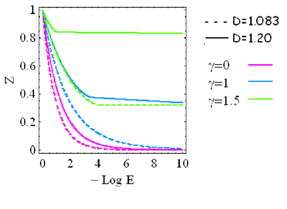
As discussed in our previous papers, near $D=1$ we find a crossover to a behavior with a sharp reduction of the quasiparticle weight in the low-energy limit. This is displayed in Fig.(2), where we have represented the electron field scale Z. If the magnetic field increases (the dashed line corresponds to B above 2 T), we have a clear signature of quasiparticles in the nonzero value of Z at low energies, whereas for vanishing $B$ the picture cannot be distinguished from that of a vanishing quasiparticle weight.

We observe from the results in Fig.(2) that the quasi- particle weight Z tends to have a flat behavior at high energies, for large values of the magnetic field $B$, (this happens because of the renormalization of the effective coupling to zero). This is in contrast to the rapid decrease signaling the typical power-law behavior, for small values of B.

The dimensional crossover approach allows us to calculate the critical exponent also in this case of a divergent interaction for $D\rightarrow 1$. In fact our target is to compare theoretical results with measurements of the tunneling DOS carried out in nanotubes when a strong magnetic field acts on them. The DOS computed at dimensions between $1$ and $2$ displays an effective power-law behavior which is given by $n(\varepsilon)\sim Z(\varepsilon)|\varepsilon|^{D-1}$, for several dimensions approaching $D=1$. Then we introduce the low-energy behavior of $Z(\varepsilon)$ in order to analyze the linear dependence of $\log(n(\varepsilon))$ on $x=-\log(\Lambda)$

$$\log(n(\varepsilon)) \approx \log{Z(\varepsilon)}+(D-1)\log(|\varepsilon|)\approx\left(\alpha_{Z}-(D-1)\right)x\equiv\alpha_{D}x.$$ (25)

Here $\alpha_{Z}$ can be easily written starting from eq.(23), if we limit ourselves to a simple first order expansion near $x=0$ with ($\log(Z)\sim\gamma(g_{0})x$), where $g_{0}$ is the initial value of the coupling (see eq(22)

$$\alpha_{Z}\approx T_{1}(\sqrt{1+g_{0}})g_{0}\frac{(3-D)f(D)(D+1)}{8}.$$ (26)

The analytic continuation in the number of dimensions allows us to avoid the infrared singularities that the long-range Coulomb interaction produces at $D=1$, providing insight, at the same time, about the fixed-points and universality classes of the theory in the limit $D\rightarrow 1$. In order to compare our results with experiments, as in ref.npb , we can obtain a lower bound for the exponent of the DOS by estimating the minimum of the absolute value of $\alpha_{D}$, for dimensions ranging between $D=1$ and $D=2$. The evaluation can be carried out starting from eq.(25) and eq.(26). We obtain a minimum value for $|\alpha_{D}|$ as a function of $D$, when we introduce the expression of $g_{0}(D,\omega_{c})$ in eq.(22).

Figure 3: (Left) The critical exponent as a function of the effective coupling $g\Xi$ obtained with a numerical calculation. (Right) Crossover dimension as a function of the effective coupling. When $B$ increases, the effective coupling is strongly reduced and the crossover dimension approaches the value $1$ according to Fig.(2), where the stability of the quasiparticle weight is reported.

The resulting value of the critical exponent $\alpha$ is

$$\alpha_{0}(\omega_{c})\approx\left(\Xi({\omega_{c}})\widetilde{g}\right)^{1/3}\approx\Xi({\omega_{c}})^{1/3}\,\alpha(0)\longrightarrow\approx\left(\Xi({\omega_{c}})\widetilde{g}\right)^{2/3}\approx\Xi({\omega_{c}})^{2/3}\,\alpha(0)$$

while in Fig.(3) we show, in the left panel, the numerical values of $\alpha$ and, in the right panel, the corresponding crossover dimension. We can observe that the growth of the magnetic field, corresponding to a reduction of the coupling $g\Xi$, reduces strongly the crossover dimension, below which the quasiparticle weight vanishes.

VI Discussion

In this paper we have described two different frameworks for dealing with the low-energy effects of the long-range Coulomb interaction in $1D$ electron systems, in order to calculate the effects of a strong transverse magnetic field. Our main focus has been the scaling behavior of quantities like the quasiparticle weight or the low-energy DOS, which can be compared directly with the results of transport experiments. For this purpose, we have developed two RG approaches: the first one at dimension $D$ strictly equal to $1$; the second one in a dimensionally regularized theory devised to interpolate between $D=2$ and $D=1$.

One of the most significant observations made in MWNTs has been the power-law behavior of the tunneling conductance as a function of the temperature or the bias voltage. The measurements carried out in MWNTs have displayed a power-law behavior of the tunneling conductance, that gives a measure of the low-energy DOS, with exponents ranging from $0.24$ to $0.37$ 22n . These values are, on the average, below those measured in SWNTs, which are typically about $0.35$ 12n . In recent papersnpb we showed that our results can account satisfactorily for this slight reduction in the critical exponent with the change of the nanotube thickness.

In a recent letter Kanda et al.kprl examined the dependence of $G$ on perpendicular magnetic fields in MWNTs. They found that the exponent $\alpha$ depends significantly on the gate voltage, giving strong oscillations. However the value of $G$ depends not only on the gate voltage, but also on the magnetic field and, in most cases, $G$ is smaller for higher magnetic fields. These authors showed that $\alpha$ is reduced from a value of $0.34$ to a value $0.11$ for a magnetic field ranging from $0$ to $4$ T, in correspondence of a peak in the $\alpha$ oscillations (and from a value of $0.06$ to a value $0.005$ for a different value of the gate voltage $V_{g}$, which corresponds to a dip in the $V_{g}$ dependence of the conductance).

Now we can compare our prediction with the experimental values starting from the strictly $1D$ approach. In order to do that, we start from eq.(17) by introducing the potential in eq.(5). It follows that a realistic value of the effective coupling at vanishing magnetic field is $U_{0}(q_{c},0)/(2\pi v_{F})\approx 8$ which gives a value for the critical exponent $\alpha\approx 0.33$. Our calculation predicts that there should be a significant reduction of $\alpha$ as the magnetic field increases for CNs of large radius. We just recall that a field $B$ of $4T$ corresponds to a value of $\gamma\approx 1$, so that the reduction of the interaction strength caused by the growth of the magnetic field gives a value of $U_{0}(q_{c},\omega_{c})/(2\pi v_{F})\approx 8/3$, which corresponds to $\alpha=0.11$, in agreement with the experimental results.

Kanda et alkprl also found a reduction at $B=0$ in the effective interaction acting on the gate voltage. In order to explain this result, we can introduce a different value of $U_{0}(q_{c},0)/(2\pi v_{F})\approx 1.42$, corresponding to the measured $\alpha=0.06$. This effect could be due to the effect of the single particle spectrumconmat and to the reduction of the Fermi velocity corresponding to a shift of the Fermi level. In this case a reduction in the coupling $U_{0}(q_{c},\omega_{c})$ of a factor $1/3$, due to the magnetic field, gives a strongest reduction in the critical exponent with $\alpha$ below $0.01$, in agreement with the measurements.

In previous papersnpb we showed that the dimensional crossover approach is appropriate for the description of CNs of large radius. There we found a value of the critical exponent in agreement with the experimental data.

As we discussed previously, the rescaling of all repulsive terms of the interaction between electrons is strongly due to the edge localization of the electrons, corresponding to a behaviour which is strictly 1D. This effect yields the result that the Luttinger liquid critical dimension (corresponding to the crossover dimension) is strongly reduced, when the magnetic field increases. A simple mechanism can explain this behavior. When $B$ increases, because of the localization of the edge states, at any dimension greater than 1 the CN is more similar to a 2D graphene sheet than to a 1D wire. Only when the energy goes below a small value, the system restores its Luttinger liquid behavior and the quasiparticle amplitude vanishes, following the usual behavior.

Hence, we predict the disappearance of the Luttinger Liquid at very strong magnetic field, and we can reduce this phenomenon to the strong localization of the edge states which imposes a 2D behaviour to the system.

It is clear from this picture that the main effect of a strong magnetic field is the fast renormalization of the coupling, which vanishes as the dimension is different from $D=1$. It follows that, for a strong magnetic field, the quasiparticle weight is not renormalized to $Z=0$ and the Luttinger liquid disappears. In this case our approach fails, because the forward scattering between currents with different chirality vanishes, coherently with the assumed formation of a chiral liquid, where obviously $\alpha$ is zero.

The main prediction that comes from our study is that there should be a significant reduction in the critical exponent of the tunneling DOS, as the transverse magnetic field is increased in nanotubes of large radius. It would be relevant to test such a dependence in experiments carried out at various values of the magnetic field, using different samples.

Appendix A From the 2D Coulomb potential to a 1D Model

We approximate the Coulomb potential function, in the limit of the small ratio $R/|y-y^{\prime}|$, as

$$U({\bf r}-{\bf r^{\prime}})=\frac{c_{0}}{|y-y^{\prime}|}\left(\sum_{k}^{\infty}\frac{{\left(-1\right)}^{k}\,\,\Gamma(\frac{1}{2}+k)}{{\sqrt{\pi}}\,\Gamma(1+k)}\left(\frac{2R}{y-y^{\prime}}\right)^{2\,k}\sin^{2\,k}(\frac{\varphi-\varphi^{\prime}}{2})\right).$$

The Forward scattering between opposite branches is obtained as

$$U(y-y^{\prime}) = c_{0}\int_{-\pi}^{\pi}d\varphi\int_{-\pi}^{\pi}d\varphi^{\prime}\sqrt{\frac{1}{(y-y^{\prime})^{2}+4R^{2}\sin^{2}(\frac{\varphi-\varphi^{\prime}}{2})}}\widetilde{\Phi^{*}}_{0,k_{F}}(\varphi,y)\widetilde{\Phi}_{0,k_{F}}(\varphi,y)\widetilde{\Phi}_{0,-k_{F}}(\varphi^{\prime},y^{\prime})\widetilde{\Phi^{*}}_{0,-k_{F}}(\varphi^{\prime},y^{\prime})$$ (27)

$$= \frac{c_{0}}{4\pi^{2}}\int_{-\pi}^{\pi}d\varphi\int_{-\pi}^{\pi}d\varphi^{\prime}\sqrt{\frac{1}{(y-y^{\prime})^{2}+4R^{2}\sin^{2}(\frac{\varphi-\varphi^{\prime}}{2})}}\left(\frac{(1-2\,{\gamma}\,\cos(\varphi^{\prime}))^{2}}{{\left(1+2\,{\gamma}^{2}\right)}}\right)\left(\frac{(1+2\,{\gamma}\,\cos(\varphi^{\prime}))^{2}}{{\left(1+2\,{\gamma}^{2}\right)}}\right)$$

$$= \frac{c_{0}}{4\pi^{2}}\sqrt{\frac{1}{(y-y^{\prime})^{2}}}\int_{-\pi}^{\pi}d\varphi\int_{-\pi}^{\pi}d\varphi^{\prime}\left(\sum_{k}^{\infty}\frac{{\left(-1\right)}^{k}\,\,\Gamma(\frac{1}{2}+k)}{{\sqrt{\pi}}\,\Gamma(1+k)}\left(\frac{2R}{y-y^{\prime}}\right)^{2\,k}\sin^{2\,k}(\frac{\varphi-\varphi^{\prime}}{2})\right)$$

$$\times \left(\frac{(1-4\,\,{\gamma}^{2}\,\cos(\varphi)\,\cos(\varphi^{\prime})+\,{\gamma}^{2}\,(\cos^{2}(\varphi)+\cos^{2}(\varphi^{\prime})))}{{\left(1+2\,{\gamma}^{2}\right)^{2}}}\right)$$

$$= 8c_{0}\sqrt{\frac{\pi^{3}}{(y-y^{\prime})^{2}}}\sum_{k}^{\infty}\frac{{\left(-1\right)}^{k}\,\,\Gamma(\frac{1}{2}+k)}{{\sqrt{\pi}}\,\Gamma(1+k)}\left(\frac{2R}{y-y^{\prime}}\right)^{2\,k}$$

$$\times \left(\frac{\Gamma(n+1/2)}{\Gamma(n+1)}-2\,{\gamma}^{2}\frac{n\Gamma(n+1/2)}{\Gamma(n+1)}+\,{\gamma}^{2}\left[\frac{\Gamma(n+1/2)}{\Gamma(n+2)}+\frac{2\Gamma(n+3/2)}{\Gamma(n+2)}\right]\right).$$

Hence, we obtain

$$U(y-y^{\prime}) = 2\frac{c_{0}}{\left(1+2\,{\gamma}^{2}\right)^{2}}\sqrt{\frac{1}{(y-y^{\prime})^{2}}}$$ (28)

$$\times \left\{K(-(\frac{2R}{y-y^{\prime}})^{2})+\frac{\pi\gamma^{2}}{4}\left(4_{2}F_{1}(\frac{1}{2},\frac{3}{2};2,-(\frac{2R}{y-y^{\prime}})^{2})+(\frac{2R}{y-y^{\prime}})^{2}_{2}F_{1}(\frac{3}{2},\frac{3}{2};2,-(\frac{2R}{y-y^{\prime}})^{2})\right)\right\}$$

where $K_{E}(x)$ gives the complete elliptic integral of the first kind, while ${}_{2}F_{1}(a,b,c,z)$ is the hypergeometric function.

The Fourier transform gives $U_{0}(q)$ as

$$U_{0}(q)=\frac{c_{0}}{\sqrt{2}\left(1+2\,{\gamma}^{2}\right)^{2}}\left[K_{0}(\frac{q}{2})I_{0}(\frac{q}{2})+{\gamma}^{2}\left(2G_{1}(\frac{q^{2}}{4})+G_{2}(\frac{q^{2}}{4})\right)\right],$$ (29)

with $K_{n}(q)$ denoting the modified Bessel function of the second kind and $I_{n}(q)$ corresponding to the modified Bessel function of the first kind. Here we have $G_{1}(z)={MeijerG}(\{\{-\left(\frac{1}{2}\right)\},\{\}\},\{\{0,0\},\{-1\}\},z)$ and $G_{2}(z)={MeijerG}(\{\{\frac{1}{2}\},\{\}\},\{\{0,1\},\{0\}\},\frac{q^{2}}{4})$, in terms of $MeijerG$ functions. The Backward scattering is obtained analogously and we obtain

$$U(y-y^{\prime}) = 2c_{0}\sqrt{\frac{1}{(y-y^{\prime})^{2}}}\left\{K(-(\frac{2R}{y-y^{\prime}})^{2})-4\pi\gamma^{2}\,_{2}F_{1}(\frac{1}{2},\frac{3}{2};2,-(\frac{2R}{y-y^{\prime}})^{2})\right\}.$$ (30)

The Fourier transform gives the $U_{0}(2k_{F})$ as

$$U_{0}(2k_{F})=\frac{c_{0}}{\sqrt{2}\left(1+2\,{\gamma}^{2}\right)^{2}}\left[K_{0}(k_{F})I_{0}(k_{F})-8{\gamma}^{2}G_{1}(k_{F}^{2})\right].$$ (31)

Appendix B Coulomb interaction in general dimension

We can start from the general Coulomb interaction in 3D and remember that the length of the system in one direction (e.g. the $x$ one) is quite smaller than in the other ($L_{y}$)

$$U({\bf r}-{\bf r^{\prime}})\approx\frac{c_{0}}{4\pi^{2}|{\bf r}-{\bf r^{\prime}}|}\left(\sqrt{\frac{L_{y}^{2}}{L_{y}^{2}+(x-x^{\prime})^{2})}}\right)=\frac{c_{0}}{|{\bf r}-{\bf r^{\prime}}|}\Upsilon_{2}(\omega_{c}),$$ (32)

where ${\bf r}$ is a $2D$ vector and

$$\Upsilon_{k,p,q}(\omega_{c})=\int\int dxdx^{\prime}\left(\sqrt{\frac{L_{y}^{2}}{L_{y}^{2}+(x-x^{\prime})^{2})}}\right)u_{0}\left(x,k\right)u_{0}\left(x,p\right)u_{0}\left(x^{\prime},(k+q)\right).u_{0}\left(x^{\prime},(p-q)\right)$$

In the limit of Forward scattering we obtain

$$\Upsilon_{F}(\omega_{c}) = \frac{1}{\left(1+\,{\gamma}^{2}\right)^{2}}$$ (33)

$$\times \left\{K(-(\frac{2R}{L_{y}})^{2})+\frac{\pi\gamma^{2}}{4}\left(4_{2}F_{1}(\frac{1}{2},\frac{3}{2};2,-(\frac{2R}{L_{y}})^{2})+(\frac{2R}{L_{y}})^{2}_{2}F_{1}(\frac{3}{2},\frac{3}{2};2,-(\frac{2R}{L_{y}})^{2})\right)\right\}.$$

References

- (1) A. Bachtold, P. Hadley, T. Nakanishi, C. Dekker, Science 294 (2001) 1317.
- (2) P.L. McEuen, Nature 393 (1998) 15.
- (3) S. Bellucci, P. Onorato, Phys. Rev. B 68 (2003) 245322. For references about the use of Quantum Wires and semiconductor devices for the spintronics, see the bibliography in this paper.
- (4) See S. Bellucci and P. Onorato, accepted by Phys. Rev. B (2005) and references therein.
- (5) T.J. Thornton, Rep. Prog. Phys. 58 (1995) 311.
- (6) J.W. Mintmire, B.I. Dunlap, C.T. White, Phys. Rev. Lett. 68 (1992) 631; N. Hamada, S. Sawada, A. Oshiyama, Phys. Rev. Lett. 68 (1992) 1579; R. Saito, M. Fujita, G. Dresselhaus, M.S. Dresselhaus, Appl. Phys. Lett. 60 (1992) 2204.
- (7) S. Tomonaga, Prog. Theor. Phys. 5 (195) 544; J. M. Luttinger, J. Math. Phys. 4 (1963) 1154; D. C. Mattis, E. H. Lieb, J. Math. Phys. 6 (1965) 304.
- (8) For a review see J. Sólyom, Adv. Phys. 28 (1979) 201, J. Voit, Rep. Prog. Phys. 57 (1994) 977.
- (9) A. De Martino, R. Egger, Europhys. Lett. 56 (2001) 570 .
- (10) V.J. Emery, in: J.T. Devreese, R.P. Evrard, V.E. Van Doren (Eds.), Highly Conducting One-Dimensional Solids, Plenum, New York, 1979.
- (11) See the first paper in TLreviwew .
- (12) F.D.M. Haldane, J. Phys. C 14 (1981) 2585.
- (13) S. J. Tans, M. H. Devoret, H. Dai, A. Thess, R. E. Smalley, L. J. Geerligs, C. Dekker, Nature 386 (1997) 474; M. Bockrath, D. H. Cobden, J. Lu, A. G. Rinzler, G. Andrew, R. E. Smalley, L. Balents, P. L. McEuen, Nature 397 (1999) 598; Z. Yao, H. W. J. Postma, L. Balents, C. Dekker, Nature 402 (1999) 273.
- (14) R. Egger, A. O. Gogolin, Phys. Rev. Lett. 79 (1997) 5082; C. Kane, L. Balents, M. P. A. Fisher, ibid. 79 (1997) 5086.
- (15) S. Tarucha, T. Honda, T. Saku, Solid State Comm. 94 (1995) 413.
- (16) A. Yacoby, H. L. Stormer, N. S. Wingreen, L. N. Pfeiffer, K. W. Baldwin, K. W. West, Phys. Rev. Lett. 77 (1996) 4612; O. M. Auslaender, A. Yacoby, R. de Picciotto, K. W. Baldwin, L. N. Pfeiffer, K. W. West, Phys. Rev. Lett. 84 (2000) 1764; M. Rother, W. Wegscheider, R. A. Deutschmann, M. Bichler, G. Abstreiter, Physica E 6 (2000) 551.
- (17) L. Balents, M.P.A. Fisher, Phys. Rev. B 55 (1997) R11973.
- (18) See the first paper in tubes .
- (19) A.O. Gogolin, Eur. Phys. J. B 3 (1998) 281.
- (20) R. Egger, H. Grabert, Phys. Rev. Lett. 79 (1997) 3463.
- (21) S. Bellucci, J. González, Eur. Phys. J. B 18 (2000) 3; S. Bellucci, Path Integrals from peV to TeV, eds. R. Casalbuoni, et al. (World Scientific, Singapore, 1999) p.363, hep-th/9810181.
- (22) S. Bellucci, P. Onorato, Phys. Rev. B 71, 075418 (2005).
- (23) S. Bellucci, J. González, P. Onorato, Nucl. Phys. B 663 [FS] (2003) 605; S. Bellucci, J. González, P. Onorato, Phys. Rev. B 69 (2004) 085404.
- (24) J. González, F. Guinea, M.A.H. Vozmediano, Nucl. Phys. B 424 (1994) 595.
- (25) S. Xu, J. Cao, C.C. Miller, D.A. Mantell, R.J.D. Miller, Y. Gao, Phys. Rev. Lett. 76 (1996) 483.
- (26) H. Ajiki, T. Ando, J. Phys. Soc. Jpn. 62 (1993) 1255.
- (27) A. Kanda et al., Physica (Amsterdam) 323 B (2002) 246.
- (28) A. Kanda, K. Tsukagoshi, Y. Aoyagi, Y. Ootuka, Phys. Rev. Lett. 92 (2004) 36801.
- (29) S. Bellucci, P. Onorato, Eur. Phys. J. B 45, 87-96 (2005).
- (30) S. Bellucci, P. Onorato, submitted to Phys. Rev. B (2005).
- (31) S. Bellucci, J. González, Phys. Rev. B 64 (2001) 201106(R).
- (32) A. Bachtold, M. de Jonge, K. Grove-Rasmussen, P.L. McEuen, M. Buitelaar, C. Schönenberger, Phys. Rev. Lett. 87 (2001) 166801;
- (33) M. Krüger, M.R. Buitelaar, T. Nussbaumer, C. Schönenberger, L. Forr , Appl. Phys. Lett. 78 (2001) 1291.
- (34) J. González, F. Guinea, M.A.H. Vozmediano, Nucl. Phys. B 406 (1993) 771.
- (35) Yu.A. Krotov, D.-H. Lee, S.G. Louie, Phys. Rev. Lett. 78 (1997) 4245.
- (36) H. J. Schulz, cond-mat/9503150.
- (37) The method of analytic continuation in the number of dimensions has been proposed in the case of a short range interaction by C. Castellani, C. Di Castro, W. Metzner, Phys. Rev. Lett. 72 (1994) 316.
- (38) P. W. Anderson, The Theory of Superconductivity in the High- Cuprates (Princeton Univ. Press, Princeton, 1997).
- (39) D. W. Wang, A. J. Millis, S. Das Sarma, report cond-mat/0010241.
- (40) See the third paper in cnts .
- (41) S. Bellucci, J. González, P. Onorato, cond-mat/0501201.