Long-range excitations in time-dependent density functional theory

Abstract

Adiabatic time-dependent density functional theory fails for excitations of a heteroatomic molecule composed of two open-shell fragments at large separation. Strong frequency-dependence of the exchange-correlation kernel is necessary for both local and charge-transfer excitations. The root of this is static correlation created by the step in the exact Kohn-Sham ground-state potential between the two fragments. An approximate non-empirical kernel is derived for excited molecular dissociation curves at large separation. Our result is also relevant for the usual local and semi-local approximations for the ground-state potential, as static correlation there arises from the coalescence of the highest occupied and lowest unoccupied orbital energies as the molecule dissociates.

I Introduction and Motivation

Time-dependent density functional theory (TDDFT) has seen a surge of applications in recent years RG84 ; PGG96 ; C96 ; MBAG02 ; MG04 ; WBG05 , with calculations of electronic excitations in a wide variety of systems of physical, chemical, and biochemical interest. Errors in TDDFT excitation energies are typically within a few tenths of an eV, while implementations can scale with size even more favorably than that of time-dependent Hartree-Fock. In principle, TDDFT yields exact excitation spectra: the errors are due to approximations to the exchange-correlation (xc) functionals. Approximations enter at two stages in usual linear response calculations: first, in the xc contribution to the one-body ground-state Kohn-Sham (KS) potential out of which bare excitations are calculated. For example, its too rapid asymptotic decay in LDA/GGA causes problems for high-lying bound states CJCS98 ; TH98b ; WMB03 ; WB05 . Second, the dynamic xc kernel must be approximated; this corrects the bare KS transitions towards the true transitions. Almost all calculations employ an adiabatic approximation, which entirely neglects frequency-dependence in the kernel. Its remarkable success for many excitations is not well understood. Understanding where it fails is important in constructing more accurate functional approximations. The lack of frequency-dependence is why adiabatic TDDFT (ATDDFT) fails for states of double excitation character MZCB04 ; CZMB04 ; C05 ; TH00 ; HH99 .

Molecular dynamics simulations, atom trapping, and photoassociation spectroscopy all need accurate calculations of excited molecular dissociation curves CGGG00 ; GGGB00 ; FR05 ; CCS98 ; WGBN04 ; LKQM05 ; fromundul , but these are challenging for approximate methods. Even ground-state dissociation is difficult FNGB05 . Closely linked are the difficulties in obtaining long-range charge-transfer (CT) excitations. The latter are notoriously underestimated in ATDDFT DWH03 ; DH04 ; T03 ; GB04b ; TAHR99 ; CGGG00 ; GGGB00 ; TTYY04 ; WV05 ; M05c , yet are vital in biological and chemical systems large enough that density functional methods are the only feasible approach.

We show here that a strong frequency-dependence in the kernel is needed near every excitation of a molecule composed of two different open-shell fragments at large separation: The ubiquitous adiabatic approximation fails for all excitations. We show this is due to static correlation in the KS ground-state, leading to every single excitation being almost degenerate with a double excitation. We resolve what the frequency-dependence of the exact xc kernel is for the tails of excited dissociation curves, and derive an approximation based on this. Our kernel yields both charge-transfer and local excitations, and contains the correct dissociation limit and leading-order polarization. It bootstraps an adiabatic approximation, and yields results to the same good level of accuracy that ATDDFT has for more common local excitations: that is, our kernel undoes the problematic static correlation in the KS system.

A crucial role is played by the step structure in the exact ground-state KS potential that develops as a heteroatomic molecule dissociates  PPLB82 ; P85b ; AB85b ; PL97c ; AB85 . The step has size equal to the difference in the ionization potentials of the two fragments, so aligns the highest occupied molecular orbitals (HOMOs) of each. Its consequences for TDDFT have only begun to be explored M05c ; LK05 . Recently we showed that near the lowest CT excitation on each fragment, the step imposes a strong frequency-dependence on the exact kernel M05c ; erratum . Here, we go much further, showing the dramatic frequency-dependence required for both higher CT and all local excitations. Local and CT excitations are intimately entangled by the step in the KS system and we construct the kernel that disentangles them.

It is important to note that although local and semi-local approximations to the ground-state potential (ie LDA and GGAs) lack the step, static correlation still features, since in these cases, the HOMO and lowest unoccupied molecular orbital (LUMO) become degenerate as the molecule dissociates. So, the construction of our xc kernel has relevant implications for the case of the usual approximate ground-state KS potentials too.

In Sec. II, we briefly review linear response theory in TDDFT. We discuss its application to CT states of a long-range molecule and point out a fundamental difference in the analysis when the closed-shell molecule consists of open-shell fragments rather than closed-shell fragments. We summarize the recent result of Ref. M05c on the structure of the exact kernel that captures the lowest CT excitations exactly in the case of open-shell fragments in the large-separation limit. In Sec. III we extend the analysis to all excitations of the molecule, showing how both local and CT excitations require strong frequency-dependence in the xc kernel that is lacking in all approximations to date. We derive an approximation to the kernel and demonstrate it on a simple molecule. Finally, Sec. IV contains a discussion on implications of our result.

II TDDFT Linear Response and Lowest Charge-Transfer States

TDDFT linear response PGG96 ; C96 proceeds by correcting the KS single excitations towards the true excitations, (which may be mixtures of any number of excitations) through the Hartree-exchange-correlation kernel $f_{\scriptscriptstyle\rm HXC}[n_{0}]({\bf r},{\bf r}^{\prime},\omega)=1/|{\bf r}-{\bf r}^{\prime}|+f_{\scriptscriptstyle\rm XC}[n_{0}]({\bf r},{\bf r}^{\prime},\omega)$, a functional of the ground-state density $n_{0}({\bf r})$. The xc kernel is the frequency-time Fourier-transform of the functional derivative of the xc potential, $f_{\scriptscriptstyle\rm XC}[n_{0}]({\bf r},{\bf r}^{\prime},t-t^{\prime})=\delta v_{\scriptscriptstyle\rm XC}({\bf r}t)/\delta n({\bf r}^{\prime}t)|_{n_{0}}$. The density-density response function of the KS system $\chi_{\scriptscriptstyle\rm S}$ and that of the interacting system $\chi$ are related through:

$$\hat{\chi}^{-1}(\omega)=\hat{\chi}_{\scriptscriptstyle\rm S}^{-1}(\omega)-\hat{f}_{\scriptscriptstyle\rm HXC}(\omega)\,.$$ (1)

Usually a matrix version C96 is used to obtain excitation energies and oscillator strengths. The vast majority of calculations utilize an adiabatic approximation for the xc kernel, i.e. one that is frequency-independent. Typically the results are accurate to within a few tenths of an eV (although there are exceptions, see eg.  TH98b ; HH99 ; CZMB04 ; DWH03 ).

When excitations are well-separated, the matrix may be simplified in a “single pole approximation (SPA)” VOC99 ; GPG00 ; AGB03 that gives the true frequency $\omega$ as a shift from a KS transition: for a closed-shell molecule,

$$\omega=\omega_{q}+2[q|f_{\scriptscriptstyle\rm HXC}(\omega_{q})|q]\,.$$ (2)

Here, $q=(i,a)$ is a double-index labeling the single KS excitation from an occupied orbital $\phi_{i}$ to unoccupied $\phi_{a}$, $\omega_{q}=\epsilon_{a}-\epsilon_{i}$, and $[q|f_{\scriptscriptstyle\rm HXC}(\omega)|q]=\int d{\bf r}d{\bf r}^{\prime}\phi_{i}^{*}({\bf r})\phi_{a}({\bf r})f_{\scriptscriptstyle\rm HXC}({\bf r},{\bf r}^{\prime},\omega)\phi_{i}({\bf r}^{\prime})\phi_{a}^{*}({\bf r}^{\prime})$.

The SPA is also an important tool in understanding the TDDFT corrections to the bare KS energies. Applying Eq. (2) to the problem of lowest charge-transfer states in a long-range molecule DWH03 , shows immediately that the correction from the kernel, $[q|f_{\scriptscriptstyle\rm HXC}(\omega_{q})|q]$, vanishes, because there is vanishing overlap between the occupied orbital $\phi_{i}({\bf r})$ on the donor and the unoccupied $\phi_{a}({\bf r})$ on the acceptor, in the limit of their large separation $R$. The TDDFT value of Eq. (2) then reduces to the bare KS eigenvalue difference, i.e. the acceptor LUMO orbital energy minus the donor HOMO orbital energy. The latter is equal to minus the ionization energy of the donor, $I_{D}$, while the former is the KS electron affinityP85b ; PL97c ; PPLB82 ; AB85 , $A_{A,\scriptscriptstyle\rm S}=A_{A}-A_{A,\scriptscriptstyle\rm XC}$, not the true electron affinity of the acceptor, $A_{A}$. The resulting frequency, $\omega=I_{D}-A_{A,\scriptscriptstyle\rm S}$, is a severe underestimate to the true CT energy: aside from the usual local/semi-local approximations underestimating the ionization energy, it lacks the xc contribution to the electron affinity, as well as the $-1/R$ tail DWH03 ; DH04 ; T03 ; GB04b . The exact CT energy is $I_{D}-A_{A}-1/R$ in the large-R limit.

When the (closed-shell) long-range molecule consists of two open-shell fragments M05c (labelled as 1 and 2 below), this argument needs to be revisited because neither the HOMO nor LUMO are localized on one of the two fragments. In the large separation limit, the exact KS potential contains a step P85b ; AB85 ; GB96 that exactly aligns the individual HOMO’s of the fragments, rendering the HOMO of the long-range molecule, $\phi_{0}$, to be the bonding molecular orbital composed of the HOMO’s of the individual fragments, $\phi_{0}=(\phi_{H,1}+\phi_{H,2})/\sqrt{2}$. The LUMO $\overline{\phi}_{0}$ is the anti-bonding molecular orbital. (See Fig.1B, and also e.g. Fig. 1 of Ref. M05c , Fig. 7 of Ref. P85b , and Fig. 1 of Ref. GB96 ). The lowest CT states lie in the subspace formed by the HOMO and LUMO, as shown by the explicit diagonalization of the Hamiltonian in Ref. M05c . Turning to TDDFT, Eq. (2), the bare KS energy difference, $\omega_{q}$, vanishes as an exponential function $e^{-R}$ of the separation of the two fragments, $R$, since the antibonding LUMO and bonding HOMO are separated in energy only by the tunnel splitting through the barrier created by the step. The correction from the xc kernel in Eq. 2 is no longer zero, as these orbitals have significant overlap in both the atomic regions. However any adiabatic approximation to the kernel will lead to drastically incorrect CT energies: The underlying reason is because the adiabatic approximation entirely neglects double-excitations MZCB04 ; CZMB04 , which are also absent in the non-interacting response function $\chi_{\scriptscriptstyle\rm S}$. Yet the double excitation to the antibonding orbital is critical in this case to capture the correct nature of the true excitations in this subspace M05c (as well as the Heitler-London ground-state). Refs. MZCB04 ; CZMB04 showed how the mixing of a double excitation with a single can be incorporated in TDDFT via a dressed SPA, $\omega=\omega_{q}+2[q|f_{\scriptscriptstyle\rm HXC}(\omega)|q]$: here the kernel has strong frequency-dependence. In Ref. M05c the form of the exact non-adiabatic xc kernel was uncovered in the limit of large separation and in the limit that the CT excitations have negligible coupling to all other excitations of the system. This was obtained by examining the structure of the response functions $\chi$ and $\chi_{\scriptscriptstyle\rm S}$ in this subspace and comparing with the explicit diagonalization of the Hamiltonian. The result was:

$$\bar{\omega}[q|f_{\scriptscriptstyle\rm HXC}(\omega)|q]=\delta^{2}+\frac{\omega_{1}\omega_{2}-\bar{\omega}^{2}}{4}+\frac{\omega_{1}\omega_{2}\delta^{2}}{\omega^{2}-\omega_{1}\omega_{2}}$$ (3)

for the KS transition $q=$bonding HOMO$\to$anti-bonding LUMO orbital. Here, $\omega_{1}=I_{2}-A_{1}-1/R$ and $\omega_{2}=I_{1}-A_{2}-1/R$, where $A=A+A_{\scriptscriptstyle\rm XC}^{\scriptscriptstyle\rm approx}$, with the xc contribution to the electron affinity of each fragment approximated as $A_{\scriptscriptstyle\rm XC}^{\scriptscriptstyle\rm approx}=-\int d^{3}r\int d^{3}r^{\prime}\phi_{H}({\bf r})^{2}\phi_{H}({\bf r}^{\prime})^{2}/|{\bf r}-{\bf r}^{\prime}|$, and $\phi_{H}$ is the HOMO of the appropriate fragment. Finally, $\delta=(\omega_{1}-\omega_{2})/2$, and $\bar{\omega}\sim e^{-R}$ is the HOMO-LUMO splitting (the bare KS frequency) M05c ; erratum . Notice the strong non-adiabaticity in the exact kernel, manifest by the pole in the denominator of Eq. (3).

The strong-frequency dependence in this expression arises due to static correlation in the system: the near-degeneracy of the antibonding orbital leads to the KS ground-state Slater determinant being near-degenerate to two others. This feature makes heteroatomic dissociation in the ground and lowest CT states resemble homoatomic dissociation in some respects GGGB00 ; problems associated with ground-state homoatomic dissociation are now well-known PSB95 . In the present paper we explore the consequences of the static correlation on all other excitations of the heteroatomic system, and model the required frequency-dependence in the kernel. Every single excitation out of the occupied bonding orbital is almost degenerate with a double excitation, where another electron is excited from the bonding orbital to the antibonding orbital . This near-degeneracy leads to strong-frequency dependence in the xc kernel relevant to all excitations of the molecule.

It is very interesting to note that although the usual local/semi-local approximations (LDA/GGA’s) to the ground-state potential do not contain the step, the HOMO and LUMO are nevertheless also delocalized over the long-range molecule. We shall return in Sec. IV to a discussion of this.

III Local and Higher Charge Transfer Excitations

Consider first a model molecule composed of two different “one-electron atoms”. At large separations, the true Heitler-London ground-state (Fig. 1A), has one electron on each atom (in orbitals $\phi_{1}$ and $\phi_{2}$ respectively). On the other hand, due to the alignment of the atomic levels caused by the step in the KS potential (Fig. 1B), the KS ground-state is the doubly-occupied bonding orbital, $\phi_{0}=(\phi_{1}+\phi_{2})/\sqrt{2}$, with each electron evenly spread over each atom. Generically, higher excitations of the atoms do not coincide; for our example, atom 2 has one higher bound excitation, whereas atom 1 has none.

Figure 1: A: Model of long-range molecule. The Heitler-London singlet ground-state is $\left(\phi_{1}({\bf r})\phi_{2}({\bf r}^{\prime})+\phi_{2}({\bf r})\phi_{1}({\bf r}^{\prime})\right)/\sqrt{2}$. The dashed curve is an excitation on “atom” 2. B: KS potential, (which eventually returns to zero on the right). The KS ground-state is the doubly-occupied bonding orbital $\phi_{0}$.

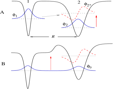
The vertical arrow in Fig. 1A illustrates a local excitation on atom 2, $\phi_{2}\to\phi_{2^{*}}$. If we attempt to describe this in the KS system, we immediately see a problem: Excitations must occur out of the occupied bonding orbital $\phi_{0}$ (Fig. 1B), so excitation leaves the molecule with “half an electron” on atom 1 and “one and a half electrons” on atom 2. This single excitation, $\phi_{0}\to\phi_{2^{*}}$ is a poor description of the excitation of the true system. The true excitation is in fact a linear combination of this single excitation and a double excitation, $(\phi_{0},\phi_{0})\to(\phi_{2^{*}},\overline{\phi_{0}})$ where the other electron occupying the bonding orbital is excited to the antibonding orbital $\overline{\phi_{0}}$ . (We assume for now the other excitations of the system are farther away in energy). Because the transition frequency to the antibonding orbital is the tunnel frequency between the atoms, it is exponentially small as a function of their separation. Thus, every single excitation of the system $(\phi_{0}\to\phi_{a})$ is almost degenerate with the double excitation $(\phi_{0},\phi_{0})\to(\phi_{a},\overline{\phi_{0}})$. This feature is a signature of static correlation in the KS ground state. Since double excitations are missing in the KS linear response MZCB04 , it is the job of the xc kernel to fold them in (see shortly).

It is instructive first to diagonalize the interacting Hamiltonian $H$ in the $2\times 2$ KS basis, whose KS energies differ only by the tunnel splitting($\sim e^{-R}$):

$$\Phi_{q} = (\phi_{0}({\bf r})\phi_{2^{*}}({\bf r}^{\prime})+\phi_{2^{*}}({\bf r})\phi_{0}({\bf r}^{\prime}))/\sqrt{2}$$

$$\Phi_{D} = (\overline{\phi_{0}}({\bf r})\phi_{2^{*}}({\bf r}^{\prime})+\phi_{2^{*}}({\bf r})\overline{\phi_{0}}({\bf r}^{\prime}))/\sqrt{2}$$ (4)

$H$ sums the kinetic, external potential, and electron interaction $(V_{\rm ee})$ operators, and rotates the pair into:

$$\Psi_{2^{*}} = \left(\phi_{1}({\bf r})\phi_{2^{*}}({\bf r}^{\prime})+\phi_{2^{*}}({\bf r})\phi_{1}({\bf r}^{\prime})\right)/\sqrt{2}$$

$$\Psi_{CT2^{*}} = \left(\phi_{2}({\bf r})\phi_{2^{*}}({\bf r}^{\prime})+\phi_{2^{*}}({\bf r})\phi_{2}({\bf r}^{\prime})\right)/\sqrt{2}$$ (5)

Within the truncated space, Eqs. (5) are eigenstates of the interacting system: $\Psi_{2^{*}}$ is a local excitation on atom 2, while $\Psi_{CT2^{*}}$ is an excited CT from atom 1 to an excited state of atom 2 (dotted arrow in Fig. 1A). Because these states are paired together due to the bonding orbital nature of the KS ground state, the two qualititatively different excitations appear together in the exact TDDFT, as we will see shortly. The eigenvalues of the diagonalization give their approximated frequencies, after subtracting the expectation value of $H$ in the Heitler-London ground-state, $E_{HL}$, (see also Refs. M05c ; MZCB04 ):

$$\omega_{2^{*}} = \epsilon_{2^{*}}-\epsilon_{2}$$

$$\omega_{CT2^{*}} = \epsilon_{2^{*}}-\epsilon_{1}-A_{\scriptscriptstyle\rm X}^{(2^{*})}-1/R\,,$$ (6)

to leading order in $R$, where

$$A_{\scriptscriptstyle\rm X}^{(2^{*})} = -\int d{\bf r}\int d{\bf r}^{\prime}\left(|\phi_{2^{*}}({\bf r})|^{2}|\phi_{2}({\bf r}^{\prime})|^{2}\right.$$ (7)

$$+ \left.\phi_{2^{*}}^{*}({\bf r})\phi_{2}^{*}({\bf r}^{\prime})\phi_{2^{*}}({\bf r}^{\prime})\phi_{2}({\bf r})\right)V_{\rm ee}({\bf r}-{\bf r}^{\prime})$$

This approximates the xc part of the excited electron affinity $A^{(2*)}$: generally for an $N$-electron species,

$$A^{*}=E_{0}(N)-E^{*}(N+1)=A_{\scriptscriptstyle\rm S}^{*}+A_{\scriptscriptstyle\rm XC}^{*}$$ (8)

with $A_{\scriptscriptstyle\rm S}^{*}=-\epsilon^{*}$, the energy of the excited KS orbital that the added electron joins. $E_{0}(N)$ is the ground-state energy of the $N$-electron system, and $E^{*}(N+1)$ is the energy of the excited state of the $(N+1)$-electron system. The excited xc electron affinity accounts for relaxation when an electron is added to an $N$-electron system, forming an $(N+1)$-electron excited state. (No correction is needed for ionization out of species 1 PL97c : the KS HOMO energy exactly equals minus the ionization potential.)

Eqs. (6) and (7) become exact in the weak interaction limit where there is no coupling to other KS excitations. Dynamic correlation is completely missing. Although derived for two one-electron atoms, the case for $N_{1,(2)}$ electrons on fragment 1(2) (both neutral and open-shell) follows analogously. Eq. (7) is an exchange approximation which may also be obtained from perturbation theory: One computes the $V_{\rm ee}$ matrix element in an $(N_{2}+1)$ electron Slater determinant, where the added electron is placed in an unrelaxed virtual orbital of the $N_{2}$-electron KS potential.

Before turning to TDDFT, we first give a simple example to test Eq. (7). We consider one fermion in a one-dimensional parabolic well MZCB04 , $H=-\frac{1}{2}\frac{d^{2}}{dx^{2}}+\frac{1}{2}x^{2}$. Excited states of two fermions in the well, interacting via a scaled delta-interaction, $V_{\rm ee}=\lambda\delta(x-x^{\prime})$, may be numerically calculated at all interaction strengths $\lambda$ MZCB04 . Figure 2 compares the affinity calculated from energy differences (Eq. 8), with Eq. (7): as expected, Eq. (7) is exact for weak interaction.

Figure 2: Exchange-correlation contribution to the excited electron affinity for a test system (See text).

Returning to TDDFT, the diagonalization process above is effectively hidden in the structure of the xc kernel. Our approximation for $f_{\scriptscriptstyle\rm XC}$ is motivated by the above analysis and also by the form of the interacting and KS density-density response functions.

Because only single excitations appear in the KS response, in a SPA $\chi_{\scriptscriptstyle\rm S}$ has one pole at $\omega_{q}=\epsilon_{2^{*}}-\epsilon_{2}$ ($\Phi_{q}$ of Eq. 4). The true density-density response however has two poles, one at the local excitation $\omega_{2^{*}}$, and the other at the CT excitation $\omega_{CT2^{*}}$. Generating an extra pole in Eq. (1) and folding in the double excitation $(\phi_{0},\phi_{0})\to(\phi_{2^{*}},\overline{\phi_{0}})$, requires a dressed (i.e. frequency-dependent) SPA (see also Ref. MZCB04 ), with the form $[q|f_{\scriptscriptstyle\rm HXC}(\omega)|q]=a+b/(\omega-c)$. Note here that $|q]=\phi_{0}({\bf r})\phi_{2^{*}}({\bf r})$. This form is consistent with the earlier diagonalization analysis (yielding Eqs. 6), which may be written

$$\omega=\langle\Phi_{q}|H|\Phi_{q}\rangle-E_{HL}+\frac{|\langle\Phi_{q}|H|\Phi_{D}\rangle|^{2}}{\omega-(\langle\Phi_{D}|H|\Phi_{D}\rangle-E_{HL})}\,,$$ (9)

A first approximation for the $f_{\scriptscriptstyle\rm XC}$ matrix element then results directly from subtracting $\omega_{q}=\epsilon_{2^{*}}-\epsilon_{2}$ from the right-hand-side of Eq. (9) (c.f. Eq. (2)). Although this would give a huge improvement over any adiabatic approximation (see later), it lacks the correct local Hartree-exchange-correlation effects. We now modify the approximation to incorporate these.

As $\langle\Phi_{D}|H|\Phi_{D}\rangle=\langle\Phi_{q}|H|\Phi_{q}\rangle+O(e^{-R})$ at large $R$, Eq. (9) suggests a two-parameter model,

$$2[q|f_{\scriptscriptstyle\rm HXC}(\omega)|q]=a-\omega_{q}+\frac{b^{2}}{\omega-a}\,.$$ (10)

We set these parameters by requiring the solutions of Eq. (2) with Eq. 10, i.e. $\omega=a\pm b$, reproduce ATDDFT values for local xc effects and for lowest order polarization. That is,

$$a=\frac{1}{2}(\omega_{2^{*}}+\omega_{CT2^{*}})\,,\,\,b=\frac{1}{2}(\omega_{2^{*}}-\omega_{CT2^{*}}),$$ (11)

where

$$\omega_{2^{*}} = \omega_{q}+\Delta_{2^{*}}+D(1,2^{*})-D(1,2)\,,{\rm and}$$

$$\omega_{CT2^{*}} = \omega_{q}+\Delta_{CT2^{*}}-\frac{1}{R}+D(1^{+},(2^{-})^{*})-D(1,2)$$

(Note again $\omega_{q}=\epsilon_{2^{*}}-\epsilon_{2}$ is the bare KS frequency). Here ATDDFT calculations on separated fragments determine all the quantities: (i) $\Delta_{2^{*}}$ is the ATDDFT value for the excitation on fragment 2, minus the KS frequency $\epsilon_{2^{*}}-\epsilon_{2}$. For example, in a SPA, $\Delta_{2^{*}}=2[q|f_{\scriptscriptstyle\rm H}+f_{{\scriptscriptstyle\rm XC},\uparrow\uparrow}^{A}|q]$, where $f_{{\scriptscriptstyle\rm XC},\uparrow\uparrow}^{A}=\delta^{2}E_{\scriptscriptstyle\rm XC}/\delta n_{\uparrow}({\bf r})\delta n_{\uparrow}({\bf r}^{\prime})$, with $E_{\scriptscriptstyle\rm XC}$ being a ground-state xc energy approximation.
(ii) $\Delta_{CT2^{*}}=-(I_{2}-I_{1})-A_{\scriptscriptstyle\rm XC}^{(2*)}$, where we write $A_{\scriptscriptstyle\rm XC}^{(2^{*})}=A(N_{2})-\omega^{*}(N_{2}+1)+\epsilon_{2^{*}}$. Here $A(N_{2})$ is the usual electron affinity of fragment 2, that may be obtained from ground-state energy differences between the negative ion formed by adding an electron to fragment 2, and that of the neutral fragment 2. The frequency of the excited state of the $(N_{2}+1)$-electron ion 2, $\omega^{*}(N_{2}+1)$, is then given by ATDDFT performed on this negative ion.
(iii) $D(1,2)$ is the dipole-dipole energy between fragment 1 and fragment 2 in their ground states; $D(1,2^{*})$ is that when fragment 2 is in the excited state; $D(1^{+},(2^{-})^{*})$ is that between the positive donor 1 in its ground state and the excited acceptor state on fragment 2. The dipole moments can either be directly obtained from the ground-state DFT densities, or extracted from ATDDFT response on separated neutral or charged fragments.

Thus we obtain the dressed kernel matrix element Eq. (10) in terms of KS quantities and ATDDFT run on the separated neutral and charged fragments.

As an example, consider two high lying excitations of the BeCl+ molecule, that dissociates in its ground state to Be⁺ + Cl. We consider the local excitation that dissociates to Be⁺(3s) + Cl(3p) and the CT excitation that is Be(3s) + Cl⁺(3p). We use the B3LYP functional for the ATDDFT pieces of the calculation, as programmed in the NWChem code nwchem . Our approximate kernel yields the tail of the Be(3s) + Cl⁺(3p) CT dissociation curve to have the frequency $(0.362-1/R)$H, and the local Be⁺(3s) excitation to be $0.394$H. These have the correct dependence up to $O(1/R^{3})$ on the separation, and the asymptotes correspond to the generally reliable ATDDFT values on the isolated Be+ and Cl fragments. On the other hand, a purely adiabatic approximation applied to the molecule yields only the local 2s$\to$ 3s excitation on Be+, with frequency $0.430$H; giving only half the usual ATDDFT correction for a local excitation on an isolated fragment (see also Sec. IV), and completely missing the CT one. Comparing with the atomic spectroscopic data of NIST for the transition frequencies nist , we find the local excitation to be $0.402$H and the CT asymptote to be $0.386$H.

IV Discussion and Outlook

Eq. (10), together with the parameters of Eq. (LABEL:eq:parameters), is our approximation for the kernel. The strong frequency-dependence is a consequence of static correlation in the KS system: our result does not go beyond the accuracy that ATDDFT has for usual local excitations, so it demonstrates the complications static correlation creates for TDDFT. The static correlation is caused by the near-degeneracy of the HOMO and LUMO orbitals due to the step in the KS potential. Our result provides a practical scheme to deal with this, constructed from ATDDFT calculations run on the individual fragments, and builds in first-order molecular polarization effects. We note that our result is only accurate for the tail end of the excited molecular dissocation curves (up to $O(1/R^{3})$). No xc effects across the long-range molecule are included. Molecular Feshbach resonances at frequencies higher than $I_{1}$ cannot be accurately described; these appear as KS shape resonances tunneling through the step. Limited in this way, and yet having complicated form, our approximation highlights challenges for a more complete description of dissociation.

There is no exponential growth of the kernel matrix element with separation, that one would expect from an adiabatic single pole analysis of long-range CT with localized (atomic)orbitals GB04b ; there the kernel would need to grow as $e^{R}$ in order to get a non-vanishing xc affinity. However, as shown here, for a long-range molecule consisting of open-shell fragments, this does not occur with the correct delocalized molecular orbitals, provided our non-adiabatic approximation is used, as the CT state is “carried along” with the local excitation, through KS excitation out of the bonding orbital.

We note that the lowest CT states in Ref. M05c , and discussed in Sec. II here, are a distinct case from the higher excitations considered here because there the underlying KS transition was nearly-degenerate with the KS ground-state itself: a single excitation to the antibonding transition $\overline{\phi}_{0}$. By perturbative arguments, the KS response goes as the inverse frequency $\sim e^{R}$. The structure of the resulting kernel (Eq. (3) in the present paper) is distinct from that for the higher local and CT excitations here (Eqs. 10 and LABEL:eq:parameters), but also displays strong frequency-dependence.

Any adiabatic approximation is stuck with unphysical half-electrons on each atom. The correction to the bare KS energy would be half of what it should be for the local excitation (since the $f_{\scriptscriptstyle\rm XC}$ matrix element involves the bonding rather than the localized orbital), and entirely misses the CT one.

The step appears in the exact ground-state KS potential, and in orbital-dependent approximations G05 . If instead LDA, or a GGA, was used for the ground-state potential, as in most calculations today, there is no step. The HOMO and LUMO are nevertheless also delocalized over the long-range molecule. It is now well-established PPLB82 ; P85b ; AB85b that the dissociation limit of the molecule places (unphysical) fractional charges on each open-shell fragment in approximations such as LDA. The individual atomic KS potentials become distorted from their isolated form in such a way as to align the individual HOMO’s with each other, yielding molecular orbitals that span the molecule, albeit unevenly. The HOMO and LUMO energies increasingly approach each other as the molecule dissociates, yielding static correlation in the long-range molecule. Clearly, in light of the results here, an adiabatic kernel used in conjunction with such a ground-state potential, will fail for all excitations, and give unphysical fractional charges on the dissociating fragments in the excited states. Frequency-dependence is needed to fold in the double-excitation associated with excitation into the LUMO. Although the result for the xc kernel of Ref. M05c , and our results in Sec. III are derived with the exact ground-state potential in mind, it may be interesting to explore the use of our kernel on top of an LDA ground-state potential, as much of the essential physics is captured. The results of this paper will be an important guide for likely modifications required in this case.

We thank the ACS Petroleum Research Fund and the National Science Foundation Career Program (CHE-0547913) for financial support, and Kieron Burke and Fan Zhang for discussions.

References

- (1) E. Runge and E.K.U. Gross, Phys. Rev. Lett. 52, 997 (1984).
- (2) M. Petersilka, U.J. Gossmann, and E.K.U. Gross, Phys. Rev. Lett. 76, 1212 (1996).
- (3) M.E. Casida, in Recent developments and applications in density functional theory, ed. J.M. Seminario (Elsevier, Amsterdam, 1996).
- (4) For many references, see N.T. Maitra et al., in Reviews in Modern Quantum Chemistry: A celebration of the contributions of R. G. Parr, ed. K. D. Sen, (World-Scientific, 2002).
- (5) M.A.L. Marques and E.K.U. Gross, Annu. Rev. Phys. Chem. 55, 427 (2004).
- (6) J. Werschnik, K. Burke, and E.K.U. Gross, J. Chem. Phys. 123, 062206 (2005).
- (7) M.E. Casida, C. Jamorski, K.C. Casida, and D.R. Salahub, J. Chem. Phys. 108, 4439 (1998).
- (8) D.J. Tozer and N.C. Handy, J. Chem. Phys. 109, 10180 (1998).
- (9) A. Wasserman, N.T. Maitra, and K. Burke, Phys. Rev. Lett. 91, 263001 (2003).
- (10) A. Wasserman and K. Burke, Phys. Rev. Lett., to appear (2005).
- (11) N.T. Maitra, F. Zhang, R.J. Cave and K. Burke, J. Chem. Phys. 120, 5932 (2004).
- (12) R.J. Cave, F. Zhang, N.T. Maitra, and K. Burke, Chem. Phys. Lett. 389, 39 (2004)
- (13) M. E. Casida, J. Chem. Phys. 122, 054111 (2005).
- (14) D.J. Tozer and N.C. Handy, Phys. Chem. Chem. Phys. 2, 2117 (2000).
- (15) S. Hirata, M. Head-Gordon, Chem. Phys. Lett., 302, 375 (1999).
- (16) F. Furche and D. Rappaport, in Computational Photochemistry, ed. M. Olivucci, (Elsevier, 2005).
- (17) M.E. Casida, K. Casida, and D. Salahub, Int. J. Quant. Chem. 70, 933 (1998).
- (18) M. Wanko et al. J. Chem. Phys. 120, 1674 (2004).
- (19) B.G. Levine et al, Mol. Phys. (2005), in press.
- (20) C. H. Greene, A.S. Dickinson, and H.R. Sadeghpour, Phys. Rev. Lett. 85, 2458 (2000).
- (21) M.E. Casida et al., J. Chem. Phys. 113, 7062 (2000)
- (22) O.V. Gritsenko, S.J.A van Gisbergen, A. Görling, and E.J. Baerends, J. Chem. Phys. 113, 8478 (2000).
- (23) see eg. M. Fuchs et al., J. Chem. Phys. (2005).
- (24) N. T. Maitra, J. Chem. Phys. 122, 234104 (2005).
- (25) A. Dreuw, J. Weisman, and M. Head-Gordon, J. Chem. Phys. 119, 2943 (2003).
- (26) D. Tozer, J. Chem. Phys. 119, 12697 (2003).
- (27) A. Dreuw and M. Head-Gordon, J. Am. Chem. Soc. 126 4007, (2004).
- (28) O. Gritsenko and E.J. Baerends, J. Chem. Phys. 121 655, (2004).
- (29) D. J. Tozer et al., Mol. Phys. 97, 859 (1999).
- (30) Y. Tawada et al., J. Chem. Phys. 120, 8425 (2004).
- (31) Q. Wu and T. van Voorhis, Phys. Rev. A. 72, 024502 (2005).
- (32) J.P. Perdew, R.G. Parr, M. Levy, and J.L. Balduz, Jr., Phys. Rev. Lett. 49, 1691 (1982).
- (33) J.P. Perdew, in Density Functional Methods in Physics, edited by R.M. Dreizler and J. da Providencia (Plenum, NY, 1985).
- (34) C.O. Almbladh and U.von Barth in Density Functional Methods in Physics, edited by R.M. Dreizler and J. da Providencia (Plenum, NY, 1985).
- (35) J.P. Perdew and M. Levy, Phys. Rev. B 56, 16021 (1997).
- (36) C.O. Almbladh and U.von Barth, Phys. Rev. B 31, 3231 (1985).
- (37) M. Lein and S. Kümmel, Phys. Rev. Lett. 94, 143003 (2005).
- (38) Note a typo in Ref. M05c : the parameter should be replaced by , as appears in Eq. (3) here.
- (39) I. Vasiliev, S. Ögüt, and J. Chelikowsky, Phys. Rev. Lett. 82, 1919 (1999).
- (40) T. Grabo, M. Petersilka, and E.K.U. Gross, in J. Mol. Structure (Theochem), 501, 353 (2000).
- (41) H. Appel, E.K.U. Gross, and K. Burke, Phys. Rev. Lett. 90, 043005 (2003).
- (42) O.V. Gritsenko and E.J. Baerends, Phys.Rev. A 54, 1957 (1996).
- (43) J.P. Perdew, A. Savin, and K. Burke, Phys. Rev. A 51, 4531 (1995).
- (44) A. Görling, J. Chem. Phys. 123, 062203 (2005).
- (45) E. Aprá, T.L. Windus, T.P. Straatsma et al., NWCHEM, A Computational Chemistry Package for Parallel Computers, Version 4.7, Pacific Northwest National Laboratory, Richland, Washington 2005; R. A. Kendall, E. Apra, D.E. Bernholdt et al., Comput. Phys. Commun. 128, 260 (2000).
- (46) “Basic Atomic Spectroscopic Data” from http://physics.nist/gov