Full optical responses of one-dimensional metallic photonic crystal slabs

Abstract

We reveal all the linear optical responses, reflection, transmission, and, diffraction, of typical one-dimensional metallic photonic crystal slabs (MPhCS) with the periodicity of a half micrometer. Maxwell equations for the structure of deep grooves are solved numerically with good precision by using the formalism of scattering matrix, without assuming perfect conductivity. We verify characteristic optical properties such as nearly perfect transmission and reflection. Moreover, we present large reflective diffraction and show that, in the energy range where diffraction channels are open, the photonic states in the MPhCS originate from surface plasmon polaritons.

Electromagnetic (EM) waves in artificial structures were one of the old problemsLord Rayleigh (1907); H. A. Bethe (1944) and had been thought to be already resolved. Since the observation of extraordinary transmission of perforated silver film in 1998,T. W. Ebbesen et al. (1998) optical responses of metallic photonic crystal slabs (MPhCS) have attracted much interest as a novel phenomenon involving surface plasmons. Many researchers have been stimulated by the phenomenon and have tried to explain the properties of transmission in MPhCS.

Even when we restrict an object to a one-dimensional (1D) MPhCS as drawn in Fig. 1, the zeroth-order transmission was already discussed in not a few reportsJ. A. Porto et al. (1999); E. Popov et al. (2000); F. J. García-Vidal and L. Martín-Moreno (2002) and explained qualitatively. In order to evaluate the transmission numerically, Maxwell equations were solved with additional assumptions such as perfect conductivity.J. A. Porto et al. (1999); F. J. García-Vidal and L. Martín-Moreno (2002) In those reports, transmission coefficient was focused on and calculated.

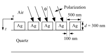
Figure 1: Structure of 1D MPhCS; the periodicity is 500 nm, the width of air slit is 100 nm, and the thickness $d$ is 300 nm. The MPhCS is on the substrate of quartz. Incident light (arrows) travels in the $xz$ plane. Incident angle $\theta$ is the angle between the normal and incident directions. The incident light is $p$-polarized.

On the other hand, diffraction has not been fully analyzed, to our best knowledge, although the surface plasmons in MPhCS are usually connected to diffraction. In fact, diffraction in optically thick metallic grooves such as Fig. 1 has been a tough subject since the first era of surface plasmons in 1980s. Maxwell equations for metallic grooves were analytically solved under the assumption of perfect conductivity;P. Sheng et al. (1982) however, the results based on the hypothesis deviate from experimental results quantitatively. Thus, there has been strong motivation for describing the optical responses of MPhCS quantitatively.

The formalism to calculate full optical response including diffraction was tried to construct, independently of the extensive studies on extraordinary transmission.M. G. Moharam et al. (1995); P. Lalanne and G. M. Morris (1996); E. Popov et al. (1986); C. D. Ager and H. P. Hughes (1991); L. Li (1996); D. M. Whittaker and I. S. Culshaw (1999) To include diffractive components, scattering-matrix (S-Matrix) formalism is suitable.E. Popov et al. (1986); C. D. Ager and H. P. Hughes (1991); L. Li (1996); D. M. Whittaker and I. S. Culshaw (1999); S. G. Tikhodeev et al. (2002) The S-Matrix method is a kind of transfer-matrix method for the propagation of EM wave. The method was invented to ensure numerical stability.D. Y. K. Ko and J. C. Inkson (1988) We adopt the S-Matrix formalism; it is based on the ordinary local response of EM fields, and the explicit expression for optical responses was presented in Ref. S. G. Tikhodeev et al., 2002. The formalism worked quite well for thin 1D gold PhCS.A. Christ et al. (2004)

In this Communication, we solve Maxwell equations for the 1D MPhCS accurately and evaluate all the linear optical responses. In particular, we explore the large diffraction and seek the physical insight. Furthermore, we discuss the physical meaning of this computation.

Figure 1 shows the structure we mainly examine here. Rectangular silver rods are infinitely long and periodically located at the 100-nm interval on the quartz substrate. Incident light is $p$-polarized, that is, the polarization of electric field is perpendicular to the axes of Ag rods. Setting $x$ axis to be the periodic direction, the electric field of $p$-polarized incident light is expanded as

$$\textbf{E}(\textbf{r},t) = \sum_{m}\textbf{E}_{m}\exp(i\textbf{k}_{m}\cdot\textbf{r}-i\omega t),$$ (1)

$$\textbf{k}_{m} = (k_{x,m},k_{y},k_{z}),$$

$$k_{x,m} = k_{x}+2\pi m/a,(m=0,\pm 1,\pm 2,\cdots),$$

$$k_{x} = k_{0}\sin\theta,$$

$$k_{z} = \sqrt{k_{0}^{2}-k_{x,m}^{2}-k_{y}^{2}}$$

where $a$ is the periodicity, $k_{0}$ is wavenumber of incident light, $\theta$ is defined in Fig. 1, and $k_{y}=0$. The electric fields in the MPhCS and substrate are expressed accordingly. The magnetic fields are described likewise. In the present S-Matrix formalism, the infinite expansion of Eq. (1) gives the Fourier-based linear equations which are exactly equivalent to Maxwell equations. Practically, the truncation of expansion is inevitable. We cut Eq. (1) at $m=\pm m_{\rm max}$ and then the total number of harmonics $N_{\rm total}$ is $2m_{\rm max}+1$. Numerical computations were executed in the highly vectorized supercomputers, which enable to make 32 parallelization. The complex dielectric constant of silver is taken from Ref. P. B. Johonson and R. W. Christy, 1972.

Figure 2: (a) Reflectance and (b) transmittance spectra of the 1D MPhCS at incident angle $\theta=0^{\circ}$.

Figure 2 displays (a) reflectance and (b) transmittance spectra calculated at incident angle $\theta=0^{\circ}$ and $N_{\rm total}=1265$. Diffraction is calculated simultaneously in this method. The fluctuation of the calculated values is within 1% for $N_{\rm total}>1200$ in this energy range.

Nearly perfect transmission at 1.2 eV in Fig. 2(b) is due to the waveguide mode in the air slit. The qualitative analysis of the mode was reported previouslyJ. A. Porto et al. (1999); E. Popov et al. (2000); F. J. García-Vidal and L. Martín-Moreno (2002) and the Fabry-Pérot nature was pointed out. The property is reproduced in our calculation. The waveguide mode does not appear above 1.7 eV where diffraction is effective, and transmission is not strongly enhanced. Reflectance is nearly 100% at 1.63 and 2.36 eV in Fig. 2(a); the response is called Wood anomaly.R. W. Wood (1902) It is usually observed at the resonances of surface plasmons in metallic grooves.

We note here the reason why the large $N_{\rm total}$ is required. This is mainly because there exist the resonances under $p$ polarization, due to the waveguide mode and surface plasmons. In a good metal such as silver, the resonances induce the spatially modulated and intense local EM fields in and near the MPhCS; the situation is in general hard to express with a small $N_{\rm total}$. Therefore, reliable numerical calculation for optical resonances requires the large $N_{\rm total}$ and actually becomes quite demanding. However, we can achieve optical responses with good precision by using a large $N_{\rm total}$ in a wide frequency range from near infrared to ultraviolet. On the contrary, in the off-resonant frequency range, far less $N_{\rm total}$ is enough to obtain the solution of Maxwell equations. Indeed, we can calculate the optical responses within 0.2% fluctuation by using a $N_{\rm total}$ of a few tens under $s$ polarization, when the polarization of electric field is parallel to the rod axes.

Figure 3(a) presents total diffraction spectrum under the normal incidence (solid line). We use the conventional notation in diffraction theory; $R_{n}$ means the $n$th reflective diffraction and $T_{n}$ the $n$th transmissive diffraction. Then, reflectance is $R_{0}$, transmittance is $T_{0}$, and the total diffraction is $\sum_{n\neq 0}(R_{n}+T_{n})$. Dashed line in Fig. 3(b) shows transmissive diffraction $\sum_{n\neq 0}T_{n}$. Similarly, the reflective diffraction $\sum_{n\neq 0}R_{n}$ is represented with dotted line.

The components of diffraction have the following properties. The transmissive diffraction $T_{\pm 1}$ emerges at 1.70 eV. The sharp onset corresponds to the opening of the first-order channel of Bragg diffraction at the interface between the quartz and MPhCS. The second channel opens at 3.40 eV and induces $T_{\pm 2}$. On the other hand, the reflective diffraction appears above 2.48 eV and is composed of $R_{\pm 1}$ in Fig. 3(b). The onset is due to the opening of the first-order channel of Bragg diffraction at the interface between the MPhCS and air. The sum of $R_{\pm 1}$ reaches the maximum of 70% at 2.75 eV. The spectra of diffraction are discussed later.

Figure 3: (a) Solid line: total diffraction spectrum of the 1D MPhCS. (b) Dashed line: transmissive diffraction. Dotted line: reflective diffraction. The sum of these diffractions is the total diffraction. The incident angle $\theta$ is $0^{\circ}$.

To examine the dispersion of resonances above 1.3 eV, we show extinction spectra at incident angle $\theta=0$ to 50 degrees in Fig. 4(a). Extinction is $-\ln(T_{0})$. The peaks of the extinction spectra are the minima of transmittance by definition and plotted with solid circles in Fig. 4(b).

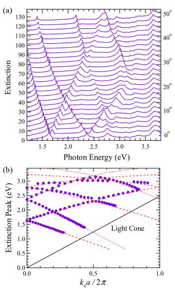
Figure 4: (a) Extinction spectra of the 1D MPhCS at incident angles from 0 to 50 degrees. (b) Dispersion relation of extinction peaks (solid circles). Dotted and dashed lines: the dispersions of reduced SPPs at the air-MPhCS and the quartz-MPhCS interfaces, respectively. The periodicity $a$ is 500 nm. The wavenumber $k_{x}$ is described in the text after Eq. (2).

We compare the dispersion of extinction with that of surface plasmon polariton (SPP). SPP at flat interface is generally expressed by

$$\omega=ck_{\parallel}\sqrt{\frac{1}{\varepsilon}+\frac{1}{\varepsilon_{\rm Ag}(\omega)}}$$ (2)

where $\omega$ is the frequency of incident light, $c$ is the velocity of light in vacuum, and $k_{\parallel}$ is wavenumber of SPP along the $x$ axis, $\varepsilon$ is dielectric constant of air or quartz, and $\varepsilon_{\rm Ag}$ is the complex dielectric constant of silver. Note that when $\varepsilon_{\rm Ag}$ is complex number, $k_{\parallel}$ is also complex. For silver in the energy range of interest, Eq. (2) holds with replacing $\varepsilon_{\rm Ag}$ by Re($\varepsilon_{\rm Ag}$) and $k_{\parallel}$ by Re($k_{\parallel}$).H. Raether (1988) We set $k_{x}=\mathrm{Re}(k_{\parallel})$ in accordance with Eq. (1). The dispersion of SPP is evaluated and shown in Fig. 4(b) after reducing into the Brillouin zone. The dotted and dashed lines represent the SPPs at the air-Ag and the quartz-Ag interfaces, respectively.

The dispersion of extinction is in good agreement with the dispersion of reduced SPPs. The agreement indicates that the reduced SPPs are resonantly excited, and strongly suggests that the photonic states in the MPhCS have formed from the reduced SPPs above 1.3 eV. The agreement is also consistent with the previous analysis with the method of rigorously coupled wave.Q. Cao and P. Lalanne (2002)

As shown in Fig. 3, the sharp onset of diffraction at 1.70 eV corresponds to the opening of $T_{\pm 1}$. On the other hand, as shown in Figs. 3 and 4, the sum of $R_{\pm 1}$ gradually increases and has the maximum at 2.75 eV; the maximum is close to the resonance of the second-order SPP at 2.80 eV and $k_{x}=0$. How can we explain the enhancement of diffraction? To extract more information, we examine the diffraction with varying only the thickness of MPhCS.

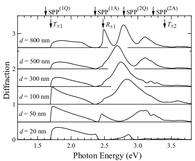
Figure 5: Total diffraction spectra at various thickness $d$. The periodicity and the width of air slit are shown in Fig. 1. The incident angle $\theta$ is $0^{\circ}$. Arrows indicate the opening of $n$th diffraction ($n=\pm 1,\pm 2$) and the resonances of SPPs. For example, SPP^(1Q) and SPP^(1A) stand for the first-order resonances at the quartz-MPhCS and air-MPhCS interfaces, respectively. The energies are taken from Fig. 4(b). The spectra at $d\geq 50$ nm are offset for clarity.

Figure 5 represents total diffraction spectra at the thickness $d=20$, 50, 100, 300, 500, and 800 nm under the normal incidence. Arrows indicate the energy positions at which the channels of diffraction open, and the resonances of reduced SPPs. SPP^(nQ) and SPP^(nA) denote the $n$th resonances at the quartz-MPhCS and air-MPhCS interfaces, respectively. The positions of SPP resonances are taken from the dispersion in Fig. 4(b). In all the spectra, diffraction arises at 1.7 eV and is comprised of $T_{\pm 1}$. At 1.7–2.4 eV, diffraction reaches a few tens of percents and the spectra show similar tendency irrespective of the thickness. Above 2.4 eV, the diffraction spectra depend on the thickness. In the thin MPhCS of $d=20$ and 50 nm, the components $T_{\pm 1}$ and $R_{\pm 1}$ coexist, and are not prominently enhanced at 2.7–2.8 eV. In the optically thick MPhCS of $d\geq 100$ nm, large peaks of diffraction appear at 2.7–2.8 eV and are dominantly composed of $R_{\pm 1}$; see Fig. 3(b) for the case of $d=300$ nm. The peak positions change with the thickness, while the extinction spectra show that the energies of SPP resonances are common in the MPhCS of $d\geq 100$ nm. Thus, though the large peaks at 2.7–2.8 eV are close to the resonance SPP^(2Q) at 2.80 eV, they cannot be simply ascribed to the resonant enhancement by reduced SPPs.

By varying the thickness from $d=20$ to 800 nm, one can observe that the diffraction spectra change in a quite complicated way. The changes in the diffraction spectra probably come from the changes of the photonic states in the MPhCS. We believe that the prominent peaks of diffraction indicate the resonant emission modes in the MPhCS.

To find the resonant modes in the MPhCS, it is a key to solve the equation of det$(\mathcal{S})=0$, where $\mathcal{S}$ is a S-Matrix for the 1D MPhCS, satisfying $|in\rangle=\mathcal{S}|out\rangle$, and $|in\rangle$ and $|out\rangle$ are input and output states, respectively. It is surely demanding and a future issue to solve det$(\mathcal{S})=0$ for a large $N_{\rm total}$. The solutions of the equation and the photonic modes were obtained for the two-dimensional PhCS made of dielectrics with a small $N_{\rm total}$.S. G. Tikhodeev et al. (2002, 2005)

We have obtained a numerically accurate solution of Maxwell equations for the 1D MPhCS and have shown the optical responses. We would like to compare the present results with measured ones quantitatively. For the precise comparison of the present calculated results with measurement, it is better to compute with using the complex dielectric constants obtained from the material used in the measurement, because the values can change under the condition of fabrication and environment.G. J. Kovacs (1978) Such comparison is a test for the validity of the ordinary local response of EM fields such as the electric flux density $\mathbf{D}(\mathbf{r})=\varepsilon(\mathbf{r})\mathbf{E}(\mathbf{r})$. If there exists definite discrepancy beyond the errors in the numerical calculation and experiment, it would be necessary to take into account the microscopic nonlocal response of EM fields.K. Cho (2003) It is an interesting subject to find the metallic nano-structures in which the nonlocal responses emerge distinctively.

In the S-Matrix formalism, one can obtain absorption $A$ by the relation of $A=1-\sum_{{\rm all}\,n}(R_{n}+T_{n})$. Thus, the absorption can be evaluated from all the components in optical measurement. The absorption spectrum is also measured directly by photoacoustic method;T. Inagaki et al. (1983); M. Iwanaga (2005) the method is useful for diffractive media.

At the end of discussion we mention the previous reports. Nearly perfect transmission, which appears at 1.2 eV in Fig. 2(b), was attributed to the waveguide mode in the slit mainly from the distribution of EM fields.E. Popov et al. (2000) The high-efficient transmission was also analyzed under the assumption of the perfect conductivity only in the slit.J. A. Porto et al. (1999); F. J. García-Vidal and L. Martín-Moreno (2002) Besides, the coupling of SPP with light was recently analyzed with extracting a effective term of S-Matrix and the transmission was explained qualitatively.K. G. Lee and Q-H. Park (2005) In this Communication, Maxwell equations for the 1D MPhCS have been solved numerically without any further technical assumption except for the inevitable truncation. From the solution, the optical responses have been evaluated directly in a wide frequency range from infrared to ultraviolet.

In conclusion, we selected typical 1D MPhCS made of silver and have computed the full optical responses precisely using the measured complex dielectric constant in the S-Matrix formalism. This is the first achievement concerning realistic calculation for 1D MPhCS with the structure of deep groove. We have confirmed the resonant excitation of reduced SPPs and found that the large reflective diffraction appears in the optically thick MPhCS. The origin has been discussed in view of resonant enhancement by reduced SPPs and of resonant emission modes in the MPhCS. The present computation, assuming the local response of EM fields, can be readily compared with measurement.