Correlated photon-pair emission from
pumped-pulsed quantum dots embedded in a microcavity

Abstract

We theoretically investigate the optical response of a quantum dot, embedded in a microcavity and incoherently excited by pulsed pumping. The exciton and biexciton transition are off-resonantly coupled with the left- and right-polarized mode of the cavity, while the two-photon resonance condition is fulfilled. Rich behaviours are shown to occur in the time dependence of the second-order correlation functions which refer to counter-polarized photons. The corresponding time-averaged quantities, which are accessible to experiments, confirm that such a dot-cavity system behaves as a good emitter of single, polarization-correlated photon pairs.

I INTRODUCTION

Semiconductor quantum dots (QDs) were recently demonstrated to emit highly nonclassical light, under proper exciting conditions Moreau et al. (2001a); Santori et al. (2002a). Besides being interesting in its own right, such phenomena can be exploited for the implementation of solid-state quantum-information devices Nielsen and Chuang (2000). Among other things, these require high collection efficiencies and photon emission rates larger than the relevant decoherence ones: two properties which are typically not present in individual QDs, but are significantly approached when the QD is embedded in a microcavity (MC). In fact, cavity photons are mostly emitted with a high degree of directionality, thus allowing for large collection efficiencies Solomon et al. (2001). Moreover, the reduction of the exciton recombination time (Purcell effect) minimizes the decoherence due to exciton-phonon scattering  Gerard et al. (1998); Solomon et al. (2001); Unitt et al. (2005); Varoutsis et al. (2005). The experimental results obtained in the low-excitation limit (i.e., at most one exciton at a time in the QD) are relatively well understood Moreau et al. (2001b); Gerard et al. (1998); Santori et al. (2001); Zwiller et al. (2002); Kiraz et al. (2002); Michler et al. (2000); Pelton et al. (2002); Fattal et al. (2004). The QD optical selection rules and its discrete energy spectrum can however be exploited also for emitting polarization-correlated photon pairs. The main goal of the present work is that of investigating the time-dependence and average values of the photon correlations, in a condition where the pair-emission probability is enhanced by suitably configuring the coupling to the MC.

The paper is organized as follows: in Sec. II we describe the system and the model we use; in Sec. III, we present the results for the time-dependent photon-coherence functions, as well as time-averaged quantities, which may directly be compared with experimental results. Finally, we drow our conclusions in Sec. IV.

II THE SYSTEM AND THE MODEL

The discrete nature of the QD energy spectra significantly reduces the portion of the dot Hilbert space which is required for the dot description, at least in the low-excitation regime. Throughout the paper, we shall accordingly restrict ourselves to the following four dot eigenstates: the ground (or vacuum) state $|G\rangle$; the two optically active single-exciton states $|X_{R}\rangle$ and $|X_{L}\rangle$, with $z$ components of the overall angular momentum $+1$ and $-1$, respectively; the lowest biexciton state $|B\rangle$. The Coulomb interaction between the carriers, enhanced by their 3D confinement, results in an energy renormalization of the exciton transitions (the so called biexciton binding energy) of the order of a few meV. These, together with the polarization-dependent selection rules, allow a selective addressing of the different transitions, already at the ps timescale (see Fig. 1). In most self-assembled QDs, the spin degeneracy of the bright exciton states is removed by the anisotropic electron-hole exchange interaction, the actual eigenstates thus being the linearly polarized $|X_{x}\rangle$ and $|X_{y}\rangle$. This geometric effect can however be compensated (e.g., by an external magnetic field), thus recovering the circularly polarized exciton basis Bayer et al. (2002). Since our goal is the efficient emission of photon pairs, we consider the QD to be embedded in a cavity having the fundamental mode with the following essential property: its frequency $\omega_{C}$ is different from the transition energies between QD states, but as close as possible to one half the energy difference between $|G\rangle$ and $|B\rangle$ ($\Delta_{1}=-\Delta_{2}$ in Fig. 1). This two-photon resonance condition seems promising for enhancing the emission of photon pairs with respect to that produced by QD’s without cavity Santori et al. (2002b); Stevenson et al. (2002); Ulrich et al. (2003, 2005). The cavity mode also presents a degeneracy with respect to the right and left polarizations. Although we do not impose any constriction on the number of photons inside the cavity, their number is limited to only a few units with the adopted range of physical parameters.

In order to account for the open nature of the cavity-dot system, we simulate its dynamics by means of a density-matrix description. In particular, the evolution of the density operator $\rho$ is given by the following master equation in the Lindblad form Scully and Zubairy (1997) ($\hbar=1$):

$$\frac{d}{dt}\rho = i\left[\rho,H_{S}\right]+\sum_{J=R,L}\frac{\kappa}{2}\left(2a_{J}\rho a^{\dagger}_{J}-a^{\dagger}_{J}a_{J}\rho-\rho a^{\dagger}_{J}a_{J}\right)+\frac{\gamma}{2}\sum_{i=1}^{4}\sum_{j=1}^{4}\left(2\sigma_{i}\rho\sigma^{\dagger}_{j}-\sigma^{\dagger}_{i}\sigma_{j}\rho-\rho\sigma^{\dagger}_{i}\sigma_{j}\right)$$ (1)

$$\times(\delta_{i,j}+\delta_{|i-j|,2})+\frac{P}{2}\sum_{n=1}^{N_{P}}\theta[t-(n-1)T+t_{P}]\ \theta[(n-1)T-t]\sum_{i=1}^{4}\sum_{j=1}^{4}\left(2\sigma^{\dagger}_{i}\rho\sigma_{j}\right.$$

$$\left.-\sigma_{i}\sigma^{\dagger}_{j}\rho-\rho\sigma_{i}\sigma^{\dagger}_{j}\right)(\delta_{i,j}+\delta_{|i-j|,2}),$$

where $a_{J}$ ($a_{J}^{\dagger}$) is the annihilation (creation) operator for a photon with polarization $J=R,L$, while $\sigma_{i=1,4}=|G\rangle\langle X_{R}|,|G\rangle\langle X_{L}|,|X_{L}\rangle\langle B|,|X_{R}\rangle\langle B|$ are the ladder operators. The second and third terms on the right-hand side of the equation account for the radiative relaxation of the cavity and of the dot, respectively; the last one corresponds to its pulsed, incoherent pumping (i.e., the electron-hole pairs being photogenerated in the wetting layer, before relaxing non-radiatively in the dot). The Hamiltonian of the coupled QD-MC system is

$$H_{S} = (\omega_{C}+\Delta_{1})\left[\mid X_{R}\rangle\langle X_{R}\mid+\mid X_{L}\rangle\langle X_{L}\mid\right]+(2\omega_{C}+\Delta_{1}+\Delta_{2})\mid B\rangle\langle B\mid$$ (2)

$$+\sum_{J=R,L}\left[\omega_{C}\left(a^{\dagger}_{J}a_{J}+1/2\right)+\sum_{i}q\left(\sigma_{i}a^{\dagger}_{J}+a_{J}\sigma^{\dagger}_{i}\right)\right].$$

In the following, we shall consider the case of degenerate excitons, while their transition energies are assumed to be detuned with respect to the cavity-mode frequency: $E_{X_{R,L}}-E_{G}=\omega_{C}+\Delta_{1}$ and $E_{B}-E_{X_{R,L}}=\omega_{C}+\Delta_{2}$. As already mentioned, we will focus on the two-photon resonance case, $\Delta_{1}=-\Delta_{2}$. Besides, the light emission through the leaky modes is considered inefficient as compared to that from the MC ($\gamma\ll\kappa$). Finally, the system is pumped by means of rectangular pulses, of intensity $P$, duration $t_{P}$, and repetition rate $1/T$.

The correlation properties of the emitted radiation are described by the first- and second-order coherence functions. Photon correlations outside the cavity can be considered proportional to those inside Walls and Milburn (1994); Stace et al. (2003). Therefore, the polarization-resolved second-order coherence functions we shall refer to in the following are:

$$g_{J,J^{\prime}}^{(2)}(t,t+\tau)=\frac{G_{J,J^{\prime}}^{(2)}(t,t+\tau)}{\langle a_{J}^{\dagger}(t)a_{J}(t)\rangle\langle a_{J^{\prime}}^{\dagger}(t+\tau)a_{J^{\prime}}(t+\tau)\rangle}\,,$$ (3)

where

$$G_{J,J^{\prime}}^{(2)}(t,t+\tau)=\langle a_{J}^{\dagger}(t)a_{J^{\prime}}^{\dagger}(t+\tau)a_{J^{\prime}}(t+\tau)a_{J}(t)\rangle\,,$$ (4)

$J,J^{\prime}=R,L$ being the photon polarizations. The dependence of the $G^{(2)}_{J,J^{\prime}}(t,t+\tau)$ on the delay $\tau$ is derived, given the system state $\rho(t)$, by means of the quantum regression theorem Scully and Zubairy (1997). Further details on the method can be found in Ref. Perea et al. (2004).

III RESULTS

III.1 Second order coherence functions

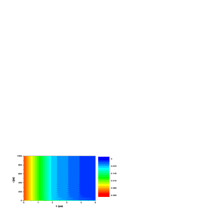
Figure 2: (Color online) Second-order coherence function $g_{L,L}^{(2)}(t,\tau)$ as a function of the two time arguments (in ps). The time origin $t=0$ is fixed at the end of the first laser pulse. The values of the physical parameters are: $q=0.1$ meV, $\kappa=0.1$ meV, $\Delta_{1}=-\Delta_{2}=0.5$ meV, $\gamma=0.01$ meV, $P=1$ meV, and $t_{P}=3$ ps.

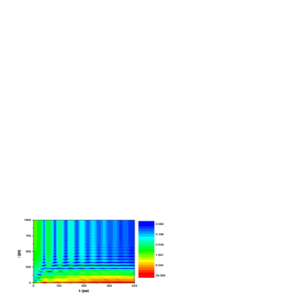
Figure 3: (Color on line) Second-order coherence function $g_{R,L}^{(2)}(t,\tau)$ as a function of the two time arguments (in ps). The values of the physical parameters are the ones reported in the caption of Fig. 2.

We start by illustrating the overall time-dependence of the second-order coherence functions, for typical values of the relevant physical parameters (specified in the figure captions), and a single excitation pulse ($N_{P}=1$). Figures 2 and 3 show $g_{L,L}^{(2)}(t,\tau)$ and $g_{R,L}^{(2)}(t,\tau)$, respectively ($g_{R,R}^{(2)}=g_{L,L}^{(2)}$ and $g_{L,R}^{(2)}=g_{R,L}^{(2)}$ due to the system’s symmetry with respect to light and exciton polarizations). The emitted light clearly exhibits non-classical features. The function $g_{L,L}^{(2)}$ quite generally shows a strongly sub-poissonian statistics [$g^{(2)}(t,0)<1$], and a clear anti-bunching behavior [$g^{(2)}(t,\tau)>g^{(2)}(t,0)$]. In fact, even though the present excitation regime is high enough for the system to be multiply excited, the polarization properties of the biexciton states and the optical selection rules suppress the probability for more than one photon to be emitted with the same polarization. Besides, due to the pulsed nature of the system’s excitation, the memory of the first photon being collected is never lost: correspondingly, the asymptotic value the $g^{(2)}(t,\tau)$ tends to for infinite delay is always well below 1, though larger than $g^{(2)}(t,0)$. The value of 1, which characterizes the continuous-pumping case Perea and Tejedor (2005), is recovered for increasing duration $t_{P}$ of the pumping pulse (not shown here). As may be expected, the features emerging from the analysis of the $g_{R,L}^{(2)}(t,\tau)$ function are quite different. In fact, the emissions of the $R$ and $L$ photons are positively correlated, and a strongly super-poissonian statistics emerges. The asymptotic values $g_{R,L}^{(2)}(t,\tau\rightarrow\infty)$, depend on the initial time $t$, whereas the overall dependence on $\tau$ includes both bunching and anti-bunching features.

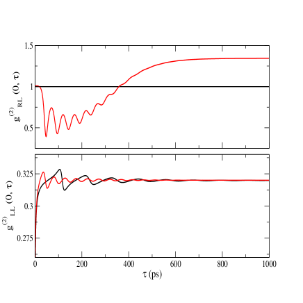
Figure 4: Color online. Second order coherence functions $g_{R,L}^{(2)}(0,\tau)$ (upper panel) and $g_{L,L}^{(2)}(0,\tau)$ (lower panel) as a function of the delay (in ps). The time $t=0$ corresponds to the end of the squared pulse (see Eq. 1). Red curves correspond to the two-photon resonance situation $\Delta_{1}=-\Delta_{2}=0.5$ meV, while the black curves correspond to a non-resonant case $\Delta_{1}=\Delta_{2}=0.1$ meV. The other parameters are $q=0.1$ meV, $\kappa=0.1$ meV, $\gamma=0.01$ meV, $P=0.1$ meV and $t_{P}=3$ ps.

In Fig. 4 we plot the functions $g_{J,J^{\prime}}^{(2)}(0,\tau)$, in order to better appreciate some of the details, and to compare the two-photon resonance case $\Delta_{1}=-\Delta_{2}=0.5$ meV with one where such condition is not fulfilled ($\Delta_{1}=\Delta_{2}=0.1$ meV). In the two-photon resonance case, $(J,J^{\prime})=(R,L)$ exhibits the above-mentioned rich behavior (upper panel): it is close to 1 (Poissonian statistics) at zero delay; it then oscillates with a pseudo period of the about 50 ps, while remaining below its initial value (photon bunching); finally, it reaches an asymptotic value of about $1.3$ (red curve).

On the contrary, for $\Delta_{1}\neq-\Delta_{2}$ (black curve), any correlation between the light emission in the two polarizations is suppressed ($g^{(2)}_{R,L}(0,\tau)=1$). The case $(J,J^{\prime})=(L,L)$ is shown in the lower panel: here, the two-photon resonance doesn’t play any role, because it doesn’t apply to two photons with the same polarization. The deep at zero delay demonstrates that the multiple excitation of each cavity mode is completely negligible, whereas that of the dot-cavity system is not (red curve): an $L$ excitation might still be transferred from the QD to the MC after an $L$ photon has been emitted at $t=0$. In this case, the differences with respect to the off-resonance case (black curve) is only due to the difference between the values of $\Delta_{1,2}$.

III.2 Two-photon coincidences

The behaviors sofar discussed are not directly accessible in experiments, for they occur on timescales which are shorter than those presently achievable, e.g., within a Hanbury-Brown-Twiss setup Scully and Zubairy (1997). In fact, the single photon detectors currently used in this kind of experiments have detection times $t_{det}$ of the order of hundreds of ps, whereas the typical timescales $G_{J,J^{\prime}}^{(2)}(t,t+\tau)$ evolves on are of tens of ps. Therefore, correlation functions have to be integrated on time intervals of the order of $t_{det}$, or larger, and normalized by analogous integrals of the populations $\langle a_{J}^{\dagger}(t)a_{J}(t)\rangle$.

Experimentally, the second-order correlation functions can be normalized by repeatedly exciting the dot by means of identical pulses, separated by time intervals $T$ of the order of $10$ ns; such a value is supposed to be much larger than any correlation time in the system. Therefore, when the start and the stop detections correspond to different pulses ($\tau>T$), no correlation at all is expected. By normalizing the second order correlation $G_{J,J^{\prime}}^{(2)}(t,t+\tau)$ with such coincidences at large delay, the value of 1 is obtained in the case of a pulsed laser Santori et al. (2002a). As a first step in the investigation of this aspect, we perform the calculation of $G_{J,J^{\prime}}^{(2)}(t,t+\tau)$, for $\tau>T$. This function is shown in Fig. 5 for $t=0$, $T=10$ ns, and all the other parameters as in Figs. 2 and 3; similar results are obtained for any other time $t$ after the first pulse.

In the following we use the above results in order to quantify the two-photon correlations. The ideal normalization of $G_{J,J^{\prime}}^{(2)}$ is given by the time integral of the uncorrelated second-order correlation function, which is given by $\langle n_{J}(t)\rangle\,\langle n_{J^{\prime}}(t+\tau)\rangle$:

$$\overline{g}_{J,J^{\prime}}=\frac{\int_{0}^{T}dt\int_{0}^{T}d\tau G_{J,J^{\prime}}^{(2)}(t,t+\tau)}{\int_{0}^{T}dt\langle a_{J}^{\dagger}(t)a_{J}(t)\rangle\int_{0}^{T}dt\langle a_{J^{\prime}}^{\dagger}(t)a_{J^{\prime}}(t)\rangle}.$$ (5)

In practice, if the dot is periodically excited by sequences of identical laser pulses, and if the time interval $T$ separating two consecutive such pulses is larger than the system’s memory, then $G_{J,J^{\prime}}^{(2)}(t,t+\tau)\simeq\langle n_{J}(t)\rangle\,\langle n_{J^{\prime}}(t+\tau)\rangle$ for $\tau>T$. Correspondingly, $\overline{g}_{J,J^{\prime}}$ can be approximated by

$$\overline{g}_{J,J^{\prime}}^{\prime}=\frac{\int_{0}^{T}dt\int_{0}^{T}d\tau\;G_{J,J^{\prime}}^{(2)}(t,t+\tau)}{\int_{t}^{T}dt\int_{T-t}^{2T-t}d\tau\;G_{J,J^{\prime}}^{(2)}(t,t+\tau)}.$$ (6)

In other words, two-photon correlation is approximated by the ratio between the areas of the first and the second peaks in Fig. 5. Our simulations of the system’s evolution under the effect of two identical squared pulses ($N_{P}=2$) aim at understanding to which extent such an approximation actually holds. Being the overall integration time $2T$ orders of magnitude larger than the characteristic timescales of the dot-cavity dynamics and, thus, of the time-step of the numerical calculations, such simulations are extremely time-consuming. In Fig. 6 we compare the values of $\overline{g}_{J,J^{\prime}}$ and $\overline{g}_{J,J^{\prime}}^{\prime}$, for different system parameters, while the time delay between consecutive laser pulses is kept constant ($T=10$ ns).

Our results show that, for small values of the dot-cavity coupling $q$, the approximation of $\overline{g}_{J,J^{\prime}}^{\prime}$ with $\overline{g}_{J,J^{\prime}}$ is not completely adequate: although the occupations of all the excited states in the system decay to negligible values on timescales of the order of $T$, the coherence function $G_{J,J^{\prime}}^{(2)}(t,t+\tau)$ still cannot be factorized, for its decay with $\tau$ is slower than that of the density matrix with $t$.

Aside from the normalization issue, a strong dependence of the second-order correlations on the dot-cavity coupling constant emerges. The value of $\overline{g}_{L,L}=\overline{g}_{R,R}$ monotonically increases with $q$, while it remains well below 1 in all the range of considered parameters. This confirms the system’s general tendency to emit not more than one photon of each polarization. In the limit of weak dot-cavity coupling, and thus of slow excitation transfer from the QD to the MC, the probability for the system to be further excited after the first photon emission has taken place is practically suppressed. In order to identify the weak and strong coupling regimes, one can make the following simple argument: the QD requires a time $\sim 1/P$ to be excited, and $\sim 1/q$ to transfer its excitation to the MC. Therefore, if $1/q\ll t_{P},1/P\sim 4$ ps, there is no time for the dot to relax by emitting a photon (in the cavity) and being subsequently re-excited by the laser pulse. In this respect, the region where $q<0.2$ meV can be identified with the weak-coupling regime.

On the other hand, $\overline{g}_{R,L}$ decreases with increasing $q$. In particular, a strong correlation is observed at the weak coupling regime, whereas the probability of an $L$ photon being emitted becomes nearly independent from the previous observation of $R$ ones ($\overline{g}_{R,L}\sim 1$) for $q\gtrsim 0.2$ meV. One could be tempted to assign some coherence properties to the regime $\overline{g}_{R,L}\sim 1$, being this the experimental value characteristic of a pulsed laser Santori et al. (2002a). However, as shown in the inset of Fig. 6, this is not the case for $g_{R,L}^{(2)}(t,t+\tau)$. In fact, the second-order coherence function shows strong and fast oscillations, indicating no coherence at all. Therefore, $\overline{g}_{R,L}=1$ cannot be identified with coherence.

IV CONCLUSIONS

We have studied the photon emission of a QD, embedded in a MC and incoherently excited by pulsed pumping. We have shown that in the two-photon resonance condition, strongly positive correlations between $R$ and $L$ radiation can be achieved, while keeping negligible the probability of emitting multiple, equally polarized photons. Under proper excitation conditions, thus, the QD behaves as an efficient emitter of counter-polarized photon pairs. The detailed analysis of the second-order coherence functions $g_{J,J^{\prime}}^{(2)}$ shows a rich behavior, including strong oscillations on a $10$ ps timescale; the asymptotic values ($\tau\rightarrow\infty$) differ from 1, the value expected in the continuous-pumping case. Time-averaged correlations $\overline{g}_{J,J^{\prime}}$ have also been computed, in order to allow a more direct comparison with experimental results. The above-mentioned features are clearly reflected also in their values, specially for small values of the dot-cavity coupling constant $q$.

V ACKNOWLEDGEMENTS

This work has been partly supported by the Spanish MCyT under contract No. MAT2002-00139, CAM under Contract No. 07N/0042/2002, and the European Union within the Research Training Network COLLECT.

Figure 1: Scheme showing the cavity-mode frequency and the QD levels. The arrows show the two types of circularly polarized optical transitions connecting the QD levels.

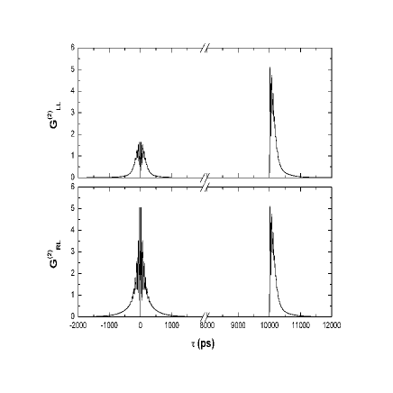
Figure 5: Non-normalized coincidences as given by $G_{J,J^{\prime}}^{(2)}(0,\tau)$ as a function of the delay (in ps) for a start time $t$ just at the end of a pulse. The two pulses are separated by $T=10$ ns. The values of the physical parameters are: $q=0.1$ meV, $\kappa=0.1$ meV, $\Delta_{1}=-\Delta_{2}=0.5$ meV, $\gamma=0.01$ meV, $P=1$ meV, and $t_{P}=3$ ps.

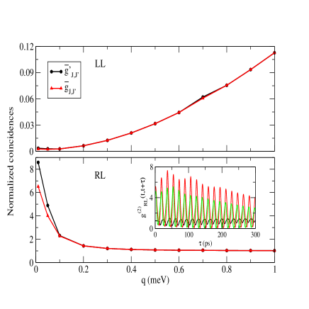
Figure 6: (Color on line) Normalized coincidences as given by $\overline{g}_{J,J^{\prime}}$ (red line) or the approximation $\overline{g}_{J,J^{\prime}}^{\prime}$ (black line) as a function of $q$. The values of the parameters are: $\kappa=0.1$ meV, $\Delta_{1}=-\Delta_{2}=0.5$ meV, $\gamma=0.01$ meV, $P=1$ meV, $t_{P}=3$ ps and $T=10$ ns. The inset shows $g_{R,L}^{(2)}(t,t+\tau)$ as a function of $\tau$ for $q=0.7$ meV and $t=0$, $50$ and $100$ ps.

References

- Moreau et al. (2001a) E. Moreau, I. Robert, J. M. Gerard, I. Abram, L. Manin, and V. Thierry-Mieg, App. Phys. Lett. 79, 2865 (2001a).
- Santori et al. (2002a) C. Santori, D. Fattal, J. Vuckovic, G. Solomon, and Y. Yamamoto, Nature 419, 594 (2002a).
- Nielsen and Chuang (2000) M. Nielsen and I. Chuang, in Quantum Computation and Quantum Information (Cambridge University Press, Cambridge, 2000).
- Solomon et al. (2001) G. S. Solomon, M. Pelton, and Y. Yamamoto, Phys. Rev. Lett. 86, 3903 (2001).
- Gerard et al. (1998) J. M. Gerard, B. Sermage, B. Gayral, B. Legrand, E. Costard, and V. Thierry-Mieg, Phys. Rev. Lett. 81, 1110 (1998).
- Unitt et al. (2005) D. C. Unitt, A. J. Bennett, P. Atkinson, D. A. Ritchie, and A. J. Shields, Phys. Rev. B 72, 033318 (2005).
- Varoutsis et al. (2005) S. Varoutsis, S. Laurent, P. Kramper, A. Lemaitre, I. Sagnes, I. Robert-Philip, and I. Abram, Phys. Rev. B 72, 041303(R) (2005).
- Moreau et al. (2001b) E. Moreau, I. Robert, L. Manin, V. Thierry-Mieg, J. M. Gerard, and I. Abram, Phys. Rev. Lett. 87, 183601 (2001b).
- Santori et al. (2001) C. Santori, M. Pelton, G. Solomon, Y. Dale, and Y. Yamamoto, Phys. Rev. Lett. 86, 1502 (2001).
- Zwiller et al. (2002) V. Zwiller, P. Jonsson, H. Blom, S. Jeppesen, M. E. Pistol, L. Samuelson, A. A. Katznelson, E. Y. Kotelnikov, V. Evtikhiev, and G. Bjork, Phys. Rev. A 66, 53814 (2002).
- Kiraz et al. (2002) A. Kiraz, S. Falth, C. Becher, B. Gayral, W. V. Schoenfeld, P. M. Petroff, L. Zhang, E. Hu, and A. Imamoglu, Phys. Rev. B 65, 161303(R) (2002).
- Michler et al. (2000) P. Michler, A. Kiraz, C. Becher, W. Schoenfeld, P. Petroff, L. Zhang, E. Hu, and A. Imamoglu, Science 290, 2282 (2000).
- Pelton et al. (2002) M. Pelton, C. Santori, J. Vuckovic, B. Zhang, G. Solomon, J. Plant, and Y. Yamamoto, Phys. Rev. Lett. 89, 233602 (2002).
- Fattal et al. (2004) D. Fattal, K. Inoue, J. Vuckovic, C. Santori, G. S. Solomon, and Y. Yamamoto, Phys. Rev. Lett. 92, 37903 (2004).
- Bayer et al. (2002) M. Bayer, G. Ortner, O. Stern, A. Kuther, A. Gorbunov, A. Forchel, P. Hawrylak, S. Fafard, K. Hinzer, T. Reinecke, et al., Phys. Rev. B 65, 195315 (2002).
- Santori et al. (2002b) C. Santori, D. Fattal, M. Pelton, G. S. Solomon, and Y. Yamamoto, Phys. Rev. B 66, 45308 (2002b).
- Stevenson et al. (2002) R. M. Stevenson, R. M. Thompson, A. J. Shields, I. Farrer, B. E. Kardynal, D. A. Ritchie, and M. Pepper, Phys. Rev. B 66, 081302(R) (2002).
- Ulrich et al. (2003) S. Ulrich, S. Strauf, P. Michler, G. Bacher, and A. Forchel, Appl. Phys. Lett. 83, 1848 (2003).
- Ulrich et al. (2005) S. Ulrich, M. Benyoucef, P. Michler, N. Baer, P. Gartner, F. J. adn M. Schwab, H.Kurze, M. Bayer, S. Fafard, Z. Wasilewski, et al., Phys. Rev. B 71, 235328 (2005).
- Scully and Zubairy (1997) M. Scully and M. Zubairy, in Quantum optics (Cambridge University Press, Cambridge, 1997).
- Walls and Milburn (1994) D. Walls and G. Milburn, in Quantum optics (Springer-Verlag, Berlin, 1994).
- Stace et al. (2003) T. M. Stace, G. J. Milburn, and C. H. W. Barnes, Phys. Rev. B 67, 085317 (2003).
- Perea et al. (2004) J. I. Perea, D. Porras, and C. Tejedor, Phys. Rev. B 70, 115304 (2004).
- Perea and Tejedor (2005) J. I. Perea and C. Tejedor, Phys. Rev. B 72, 35303 (2005).