Calculation and spectroscopy of the Landau band structure at a thin and atomically precise tunneling barrier

Abstract

Two laterally adjacent quantum Hall systems separated by an extended barrier of a thickness on the order of the magnetic length possess a complex Landau band structure in the vicinity of the line junction. The energy dispersion is obtained from an exact quantum-mechanical calculation of the single electron eigenstates for the coupled system by representing the wave functions as a superposition of parabolic cylinder functions. For orbit centers approaching the barrier, the separation of two subsequent Landau levels is reduced from the cyclotron energy to gaps which are much smaller. The position of the anticrossings increases on the scale of the cyclotron energy as the magnetic field is raised. In order to experimentally investigate a particular gap at different field strengths but under constant filling factor, a GaAs/AlGaAs heterostructure with a 52 Å thick tunneling barrier and a gate electrode for inducing the two-dimensional electron systems was fabricated by the cleaved edge overgrowth method. The shift of the gaps is observed as a displacement of the conductance peaks on the scale of the filling factor. Besides this effect, which is explained within the picture of Landau level mixing for an ideal barrier, we report on signatures of quantum interferences at imperfections of the barrier which act as tunneling centers. The main features of the recent experiment of Yang, Kang et al. are reproduced and discussed for different gate voltages. Quasiperiodic oscillations, similar to the Aharonov Bohm effect at the quenched peak, are revealed for low magnetic fields before the onset of the regular conductance peaks.

I Introduction

The bending of the Landau levels at the edge of a two-dimensional electron system (2DES) is a well-investigated field, since it represents an essential ingredient for the explanation of the quantum Hall effect.Halperin (1982); MacDonald and Středa (1984); Chklovskii et al. (1992) Generally, one has been dealing with a confining potential much wider than the magnetic length. Only with the technique of cleaved edge overgrowth (CEO)Pfeiffer et al. (1990) it became possible to define a sharp edge potential on the atomic scale.Huber et al. (2005) Kang, Yang and co-workersKang et al. (2000); Yang et al. (2004, 2005) used this technique to separate a 2DES laterally by a $88\ \text{\AA}$ wide and $212\ \text{meV}$ high barrier. Using modulation doping, they achieved electron densities of $1.1$ and $2.0\times 10^{11}\ \text{cm}^{-2}$. Variation of the magnetic field and the bias voltage was employed to investigate the Landau band structure. Although the experiment of Kang et al. reveals the principal features expected for the setup very well, there are some points which are hardly explainable in the picture of Landau level mixing. In particular, the first conductance peak for zero bias occursKang et al. (2000) at filling factor $\nu=1.2$ while the dispersion predicts $\nu\approx 4$. Furthermore, instead of the observed broad conductance peaks, the small energy gaps in the single electron picture would suggest very sharp peaks. The latter phenomenon was discussed in several publications.Mitra and Girvin (2001); Kollar and Sachdev (2002); Takagaki and Ploog (2000); Zülicke and Shimshoni (2003); Kim and Fradkin (2003) The consideration of Coulomb interactionsMitra and Girvin (2001); Kollar and Sachdev (2002) leads to wider gaps which predict conductance peaks ($\Delta\nu\approx 0.01$) of still considerably smaller width than detected in the experiment ($\Delta\nu\approx 0.15$). While this effect was also observed, we shall focus here on the dependence of the peak position on the magnetic field. In addition to the regular oscillations we shall investigate quasiperiodic structures of the conductance at low magnetic fields and at the $\nu\approx 2$ peak.

Section II discusses the analytical solution of the Schrödinger equation for the coupled system which is outlined in Fig. 1. The wave functions are represented by parabolic cylinder functions giving a convenient expression as a good starting point when expanding the single electron model to an interacting model. With the presented method, the dispersion can be determined for different sets of parameters, especially for the strong coupling regime where the picture of overlapping Landau bands as obtained at an infinitely high barrier is not valid.

With our experiment (Sec. III) we want to get further insight into the correspondence of the energy dispersion with the conductance. Controlling the Fermi level allows us to investigate the same gap at different magnetic fields. As a consequence, instead of preparing samples with a thin AlGaAs layer of different thickness, the magnetic field can be used to tune the effective shape of the barrier while the filling factor is kept constant by means of the gate electrode. The advantage of providing variable electron densities with one sample is furthermore that small effects due to unavoidable fluctuations between successive growth processes can be excluded. This is essential when considering quantum interferencesYang et al. (2005); Kim and Fradkin (2003) at tunneling centers caused by imperfections of the barrier. With increasing electron density, a shift of the conductance peaks towards higher filling factors is observed which can be explained partly by the rise of the band gaps on the scale of the cyclotron energy. While important properties like the distortion of the $\nu\approx 2$ peak by irregular large-period featuresYang et al. (2005) are reproduced with our sample, there are substantial differences compared to the modulation-doped structure of Kang and co-workers. The oscillations highly exceed the expected limit by the conductance quantum, and the peaks are separated about twice the distance on the scale of the filling factor.

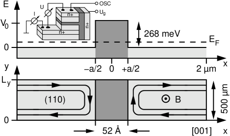
Figure 1: Shape of the conduction band edge and sketch of both 2DESs. The latter reside in two GaAs layers grown during the first MBE step on a (001) wafer. The tunneling barrier consists of about 18 monolayers of $\text{Al}_{0.34}\text{Ga}_{0.66}\text{As}$. The trajectories represent the two outermost edge channels. The inset depicts our sample structure.

II Band structure

The goal of this section is to calculate the exact dispersion of a single electron in the vicinity of the tunneling barrier by determination of its eigenstates in the whole sample region composed of both electron systems and the barrier. The spin is not considered here. The time-independent Schrödinger equation $H\psi=E\psi$ in the effective mass approximation,

$$\left[\frac{1}{2m}\left(\mathbf{p}+e\mathbf{A}\right)^{2}+V(x)\right]\psi(x,y)=E\psi(x,y),$$ (1)

has to be solved where $V(x)$ is the conduction band offset as shown in Fig. 1. For both materials the same effective mass of $m=0.067\ m_{e}$ has been used. Neglecting all other edge potentials, we are assuming infinitely extended electron systems in the $x$-direction and periodic boundary conditions for the $y$-direction. At first, the most general solution of (1) for a region with constant $V(x)$ is determined, and then, by applying the continuity conditions at the barrier, the eigenenergies are calculated numerically. The symmetry of the system suggests the Landau gauge $\mathbf{A}=(0,xB,0)$ which yields the Hamiltonian

$$H=\frac{\hbar^{2}}{2m}\left[\left(\frac{1}{i}\frac{d}{dy}+\frac{x}{\ell^{2}}\right)^{2}-\frac{d^{2}}{dx^{2}}\right]+V(x),$$

where $\ell=\sqrt{\hbar/eB}$ is the magnetic length. The corresponding Schrödinger equation is solved by the ansatz $\psi(x,y)\propto e^{iky}\varphi(x)$. The wave function is localized in the $x$-direction and depicts a plain wave parallel to the barrier with momentum $k\in\mathbb{Z}\times 2\pi/L_{y}$. This results in the one-dimensional differential equation

$$\frac{\hbar\omega_{c}}{2}\left[\left(k\ell+\frac{x}{\ell}\right)^{2}-\ell^{2}\frac{d^{2}}{dx^{2}}+\frac{2V(x)}{\hbar\omega_{c}}\right]\varphi(x)=E\varphi(x).$$

In the following, the individual bands of the dispersion are indexed by the Landau level number $n$. It is convenient to define the dimensionless energy $\varepsilon_{nk}$ by

$$E_{nk}=\left(\varepsilon_{nk}+\textstyle\frac{1}{2}\right)\hbar\omega_{c}.$$

Figure 2: Parabolic cylinder function. When $\varepsilon$ approaches the integral value $n=5$, the divergence shifts to the left until it disappears completely.

The guiding center of the wave function is given by $X=-k\ell^{2}=-\hbar k/eB$. The parameters $\xi=(x-X)/\ell$ and $v=V/\hbar\omega_{c}$ are introduced in order to get an equation which depends only on dimensionless variables and whose solution can be found in the literature on higher transcendental functions:Erdélyi et al. (1953); Magnus et al. (1966); Bartoš and Rosenstein (1994)

$$\left[\frac{d^{2}}{d\xi^{2}}-\xi^{2}+2\left(\varepsilon_{nk}-v(\xi)+\frac{1}{2}\right)\right]\varphi_{nk}(\xi)=0.$$

Within regions of constant $v(\xi)$ the solution space is spanned by two parabolic cylinder functions:

$$\varphi_{nk}(\xi)=\gamma_{1}D_{\varepsilon_{nk}-v}(\xi\sqrt{2})+\gamma_{2}D_{\varepsilon_{nk}-v}(-\xi\sqrt{2}).$$

The function $D_{\varepsilon}(z)$ is plotted in Fig. 2 for several parameters. At integer values of the energy, $\varepsilon_{nk}=n$, the parabolic cylinder function converges overall and it holds $D_{n}(\xi\sqrt{2})=2^{-n/2}e^{-\xi^{2}/2}H_{n}(\xi)$. This is the solution of the harmonic oscillator which is valid for bulk states. Their orbit center $X$ coincides with the center of the wave function and its distance to the barrier is at least about $(n+1)\ell$. For a non-integer value of $\varepsilon$ the function $D_{\varepsilon}(z)$ diverges when its argument goes to minus infinity. Thus for the right 2DES $\gamma_{2}$ has to be set to zero while the wave function in the left electron system is $\varphi_{nk}(\xi)\propto D_{\varepsilon_{nk}}(-\xi\sqrt{2})$. The general solution of (1) is then given by

$$\psi_{nk}(\xi,y)=e^{iky}\\ \times\begin{cases}D_{\varepsilon_{nk}}(-\xi\sqrt{2})&\phantom{|}x\phantom{|}<-a/2\\ D_{\varepsilon_{nk}-v}(\xi\sqrt{2})+\beta_{nk}D_{\varepsilon_{nk}-v}(-\xi\sqrt{2})&|x|\leq\phantom{-}a/2\\ D_{\varepsilon_{nk}}(\xi\sqrt{2})&\phantom{|}x\phantom{|}>-a/2.\end{cases}$$ (2)

For simplicity all prefactors have been dropped. The characteristic parameters of the system are $V_{0}$, $a$, and $B$, but the shape of the dispersion $\varepsilon_{n}(X/\ell)$ is just determined by the effective height $v$ and width $a/\ell$ of the barrier.

Figure 3: Two-dimensional parameter space $(\varepsilon_{n},\beta_{n})$ for $B=9.2\ \text{T}$, the orbit center $X=-1.8\,\ell$, and a barrier of the height $v=3$ and width $a=179\ \text{\AA}=2.12\,\ell$. For each point on the dashed (solid) curve the boundary condition (5) on the right (left) side of the barrier is fulfilled. So the crossing points ($\circ$) represent the eigenstates of the system while pseudo solutions ($\square$) correspond to a vanishing denominator in (6).

Both unknown variables, the energy $\varepsilon_{nk}$ and the mixing ratio $\beta_{nk}$ of the parabolic cylinder functions inside the barrier, are determined by the boundary conditions at the interfaces of the barrier. The continuity of the wave function and its derivative is fulfilled when $d\,\log\varphi_{nk}(\xi)/d\xi$ is constant at the left ($-$) and right ($+$) side of the potential elevation:

$$\left.\begin{gathered}\frac{d}{d\xi}\log D_{\varepsilon_{n}}(\pm\xi\sqrt{2})=\\ \frac{d}{d\xi}\log\left[D_{\varepsilon_{n}-v}(-\xi\sqrt{2})+\beta_{n}D_{\varepsilon_{n}-v}(\xi\sqrt{2})\right]\end{gathered}\right|_{\,\displaystyle\xi=\xi_{\pm}}$$ (5)

$$\text{with}\quad\xi_{\pm}=\pm\frac{a}{2\ell}-\frac{X}{\ell}.$$

The evaluation of these expressions yields withErdélyi et al. (1953) $D^{\prime}_{\varepsilon}(z)=\frac{z}{2}D_{\varepsilon}(z)-D_{\varepsilon+1}(z)$ the following two equations:

$$\begin{aligned} &\mp D_{\varepsilon_{n}+1}(\pm\xi_{\pm}\sqrt{2})D_{\varepsilon_{n}-v}(-\xi_{\pm}\sqrt{2})\\ &\quad\mp\beta_{n}D_{\varepsilon_{n}+1}(\pm\xi_{\pm}\sqrt{2})D_{\varepsilon_{n}-v}(\xi_{\pm}\sqrt{2})\\ &\quad-D_{\varepsilon_{n}}(\pm\xi_{\pm}\sqrt{2})D_{\varepsilon_{n}-v+1}(-\xi_{\pm}\sqrt{2})\\ &\quad+\beta_{n}D_{\varepsilon_{n}}(\pm\xi_{\pm}\sqrt{2})D_{\varepsilon_{n}-v+1}(\xi_{\pm}\sqrt{2})\end{aligned}\quad\qquad$$ (6)

$$\frac{}{D_{\varepsilon_{n}}(\pm\xi_{\pm}\sqrt{2})\Bigl{(}D_{\varepsilon_{n}-v}(-\xi_{\pm}\sqrt{2})+\beta_{n}D_{\varepsilon_{n}-v}(\xi_{\pm}\sqrt{2})\Bigr{)}}=0.$$

Finding all solutions in the ranges $\varepsilon_{nk}\in\left[0;\varepsilon_{\text{max}}\right]$ and $\beta_{nk}\in\left[-\infty;+\infty\right]$ requires some effort beyond standard algorithms for equation systems. At fixed $X$ the numerators of (6) are solved separately for $\beta_{nk}^{(+)}$ and $\beta_{nk}^{(-)}$ as shown in Fig. 3. For $(\varepsilon_{nk};\beta_{nk})=(v;-1)$, $(v+1;1)$, $(v+2;-1)$, $\ldots$ both the numerators and denominators vanish. Apart from these pseudo solutions all other crossings have to be found to obtain the energy dispersion. This is intricate due to partly very small singularities and high-valued regions of $\beta_{nk}^{(\pm)}(\varepsilon_{nk})$.

Figure 4: Dispersion relation (solid lines) for a low barrier. The parameters are the same as in Fig. 3. For comparison, the eigenstates for an infinitely high barrier are plotted as dashed curves. The lowest gap inside the barrier is only $0.08\,\hbar\omega_{c}$ wide. The dash-pointed line denotes the barrier.

The results for the case of strongly coupled electron systems are shown in Fig. 4 where the barrier has a height on the order of the cyclotron energy. Just like the wave functions themselves (Fig. 2), with subsequent index $n$ an additional oscillation appears in the band $\varepsilon_{nk}$. While the gap between the two lowest Landau bands is very small, it rises up to the order of $\hbar\omega_{c}$ for eigenstates lying energetically above the barrier. The depicted dispersion for an infinitely high barrier is obtained for the left 2DES by solving $D_{\varepsilon_{nk}}\left(\sqrt{2}(\frac{a}{2}+X)/\ell\right)=0$. The wave function is given by (2) with a vanishing amplitude for $|x|\leq a/2$. A different ansatz in Ref. MacDonald and Středa, 1984 yields the same result. The overlapping Landau bands can be used as a basis for further perturbation calculations. In contrast to the situation in Fig. 4 this works well only when the appropriate Landau band lies significantly below the barrier.

Figure 5: Band structure for our sample with $V_{0}=268\ \text{meV}$ and $a=52\ \text{\AA}$. (a) The points are the result of the complete quantum-mechanical calculation, and the solid lines are corresponding to an infinitely high barrier. The magnetic shift and the gaps are resolved by magnifying the marked rectangular region: (b) Here, the bold lines stand for the overlapping Landau bands of two 2DESs separated by an infinitely high barrier. The crossing shifts by $\Delta\varepsilon=0.05$ when the magnetic field increases as denoted. The anticrossing below (thin lines) divides the second and third Landau levels of the coupled system. With the change of $B$, the size of the gap rises from $0.013$ to $0.016\,\hbar\omega_{c}$ while its position shifts by $\Delta\varepsilon=0.02$ (see also Table 1).

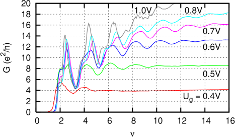
Figure 6: (Color online) Magneto-oscillations of the tunneling current at $400\ \text{mK}$. The conductance $G=I/V$ is plotted against the filling factor for several gate voltages $U_{g}$.

In order to suppress the bulk leakage current in our sample structure (Fig. 1), a rather high barrier with $V_{0}\gg\hbar\omega_{c}$ at typical field strengths was used. The corresponding band structure of the weakly coupled system is shown in Fig. 5 for two different magnetic fields. The deviation from the dispersion at an infinitely high barrier is quite small, in contrast to the situation in Fig. 4. But in detail, when looking at the dependence of the gap positions on the magnetic field as demonstrated in Fig. 5(b), the need for the outlined numerical solution is apparent. This predicts a shift of $\Delta\varepsilon=0.02$ which amounts about half the value than given by the superposition of two opposing Landau bands, because for an increasing magnetic field not only the rising effective barrier width $a/\ell\propto\sqrt{B}$ is considered but also the compensation by the decrease of its effective height $v\propto 1/B$. For the same reason, at increasing magnetic field, the coupling between the opposite edge channels is intensified which leads to energy gaps rising faster than the cyclotron energy. The investigation of the gap position on the scale of the Landau level order is in the main focus of our experiment.

III Experiment

The heterostructure shown in Fig. 1 was fabricated in two steps by employing the cleaved edge overgrowth method described in detail in Ref. Pfeiffer et al., 1990. During a first growth process the $a=52\ \text{\AA}$ thick tunneling barrier, two intrinsic regions (each $2\ \mu\text{m}$), where the electron systems reside, and two highly doped contact layers were produced. Immediately after cleaving the sample in situ, a gate structure with a $d=100\ \text{nm}$ thick barrier and a $200\ \text{nm}$ $\text{n}^{+}$-contact layer was grown on the freshly exposed (110) cleavage plane. This design allows the variation of the electron density, but the induced 2DESs cannot be contacted by a true four-point method.

While applying a magnetic field perpendicular to the cleavage plane, the conductance was measured with lock-in technique using a $10\ \text{nA}$ sinusoidal current at $17\ \text{Hz}$. In Fig. 6 the conductance is plotted versus the filling factor $\nu=nh/eB$ in order to allow direct comparison for different electron densities. As the electron density $n$ cannot be measured directly, it is determined from the periodicity of the tunneling resistance over $1/B$, see Fig. 7. Takagaki and PloogTakagaki and Ploog (2000) already confirmed for this kind of tunneling spectroscopy an equidistant conductance peak separation, namely, with a distance of $\Delta\nu=2$ for a spin-degenerate system. Indeed, a constant interval is also found experimentally at high accuracy as demonstrated in Fig. 9. In addition, the determined densities are in agreement with by the capacitor model

$$n(U_{g})=\frac{\epsilon_{r}\epsilon_{0}}{de}\left(U_{g}-U_{0}\right)$$ (7)

for the gate structure. Under low gate leakage, $n(U_{g})$ fits well to the experimental data when the dielectric constantSadao (1994) $\epsilon_{r}=11.6$ for $\text{Al}_{0.34}\text{Ga}_{0.66}\text{As}$ at $0\ \text{K}$ and the sample specific offset $U_{0}$ are used. For voltages $\gtrsim 0.6\ \text{V}$ an appreciable gate leakage current emerges. The upper electron system depletes as the electron supply from ground is restricted by the $52\ \text{\AA}$ tunneling barrier. The 2DESs are therefore shifted against each other by an internal bias $U_{2}$ which is also plotted in Fig. 7.

Figure 7: Electron density obtained by analyzing the resistance traces in the same way as is customary for Shubnikov-de Haas oscillations. The density increases linearly until saturation effects appear at $U_{g}=0.7\ \text{V}$. The relation (7), $n=5.85\times 10^{11}\,(U_{g}-0.18\ \text{V})\ \text{cm}^{-2}/V$, is plotted with a fitted offset $U_{0}$ as the dashed line. The solid line represents the potential $U_{2}$ of the upper contact layer (Fig. 1).

In the picture of Landau level mixing, Kang and co-workersKang et al. (2000) explained the oscillatory structure of the conductance by the periodic appearance and disappearance of the inner counterpropagating edge channels along the barrier (Fig. 1) as the Fermi level is varied. When the latter enters one of the small gaps, which divide subsequent Landau bands, see Fig. 5(b), the corresponding edge channels vanish while still remaining at the other edges of the sample. By tunneling over the barrier, one large edge channel spanning the whole sample is formed which gives rise to a conductance peak.

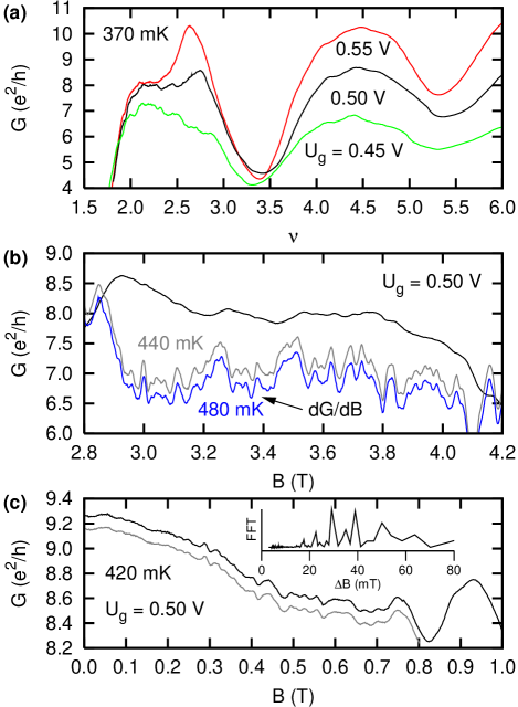
Figure 8: (Color online) Some features of the conductance traces. (a) First two conductance peaks at different gate voltages. (b) The magnification of the quenched peak around $\nu=2.5$—now plotted against the magnetic field—shows irregular oscillations, more clearly seen on its derivative which is reproduced for two subsequent magnetic field sweeps. (c) Small-period oscillations at low magnetic fields are also highly reproducible at different field sweeps. The fast Fourier transform reveals about two distinct periods.

Although a four-point measurement was carried out, the interrupted electron system is effectively contacted via two points, namely, by two extended $\text{n}^{+}$-layers. Consequently, in the quantum Hall regime the conductance is expected to increase at most by two conductance quanta when the tunneling of an edge channel is switched on. Several edge channels may be involved at higher filling factors so that this limit can be exceeded.Takagaki and Ploog (2000) In contrast to Refs. Kang et al., 2000; Yang et al., 2004, 2005, where amplitudes on the order of $0.1\ e^{2}/h$ are reported, we see conductance peaks with a height of about $10\ e^{2}/h$, even at $\nu\approx 2$. The conductance varies from sample to sample, and when investigating a sample which is half as wide, both the absolute conductance at vanishing magnetic field and the amplitude of the magneto-oscillations are reduced by the factor $1.8\pm 0.2$ compared to a $500\ \mu\text{m}$ sample obtained from the same growth. The tunneling barrier faces to both highly doped contact layers which are $250$ or $500\ \mu\text{m}$ long and reside at a distance of $2\ \mu\text{m}$. Despite the extreme proportions of the 2DESs, the enhancement of the conductance cannot be explained by backscattering effects due to impurities since the magnetic length is still much smaller than the width of the electron systems. It rather seems that several macroscopic defects separate the active region perpendicularly to the tunneling barrier into independent sections. The formation of multiple edge channels in parallel overrides the limit of $2\ e^{2}/h$. There is a couple of possible origins for these defects. Small oval defects do not affect the lateral transport of a (100)-2DES in the quantum Hall regime, but when randomly cleaved during the CEO process, they massively distort the active region. The same applies to low corrugations and steps arising when the sample does not cleave perfectly, and partial damages of the unprotected upper edge of the cleavage plane during processing are also responsible for the separation. A direct comparison of the conductance amplitude with the values of Refs. Kang et al., 2000; Yang et al., 2004, 2005 is not reasonable as the number of independent sections is not available and, in addition, the contact resistance and the tunneling properties of the barrier had to be known for explaining any differences. The barrier of Kang et al. was realized in a different way, namely, as an $88\ \text{\AA}$ thick digital alloy of $\text{Al}_{0.1}\text{Ga}_{0.9}\text{As}$/AlAs, and the contacts were made by means of photolithography.

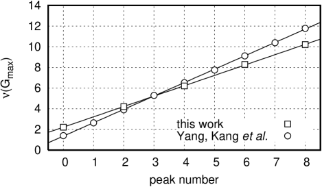
Figure 9: Position of the conductance peaks on the scale of the filling factor; $\square$, peaks shown in Fig. 6 at $U_{g}=0.5\ \text{V}$ with $n=1.87\times 10^{11}\ \text{cm}^{-2}$; $\circ$, data presented in Fig. 1a of Ref. Yang et al., 2004. The density $n=1.89\times 10^{11}\ \text{cm}^{-2}$ is obtained from $R_{xx}(B)$ which is also plotted there. Straight lines: least mean square fit to the data points.

Even though our sample differs in considerable points, it displays an important feature also discovered in the earlier experiments.Yang et al. (2005) For a non-biased system the leftmost peak in Fig. 8(a) is substantially cropped, and the peak at $\nu=4.5$ is also distorted. With increasing gate voltage, a smooth peak emerges from the quenched peak at the left and the oscillatory structure of the right peak becomes slightly weaker. While in Ref. Yang et al., 2005 a similar effect was reported for the application of an external bias, in our sample the internal bias due to gate leakage is responsible for the suppression of the irregular oscillations: it increases in Fig. 8(a) from $0.2$ to $2\ \text{mV}$. The quenched peak, cf. Fig. 8(b), consists of a superposition of two different types of oscillatory features. The first one has a large period of about $0.23\ \text{T}$ and can be seen in $G(B)$ at rather high temperatures. The origin of these oscillations remains unclear. However, small-period oscillations which appear at dilution refrigerator temperatures were identified in Ref. Yang et al., 2005 as Aharonov-Bohm (AB) oscillations. They occur due to strong coupling of the counterpropagating edge states via imperfections in the barrier. Although the AB effect is supposedYang et al. (2005) to be strongly suppressed above $200\ \text{mK}$, we can reveal the oscillations still at $480\ \text{mK}$ by averaging and differentiating as shown in Fig. 8(b). They are quasiperiodic with not very distinct periods in the range of $\Delta B=40\ldots 70\ \text{mT}$. This corresponds to a distance of $h/ea\Delta B=7\ldots 12\ \mu\text{m}$ between adjacent interference slits in the barrier. Following from the average distance of the tunnel sites, a lower bound of the phase-coherent length for the edge channels along the barrier is estimated at $l_{\Phi}\approx 20\ \mu\text{m}$. The AB oscillations cannot be detected for the $\nu\geq 4.5$ peaks. Before the onset of the regular conductance peaks at about $B=0.8\ \text{T}$, see Fig. 8(c), a series of small quasiperiodic oscillations exists whose periods of $30{-}50\ \text{mT}$ are independent of the field magnitude. With increasing electron density, the emergence of these oscillations decreases from $0.37\ \text{T}$ at $U_{g}=0.45\ \text{V}$ to $0.20\ \text{T}$ at $U_{g}=0.55\ \text{V}$ as the mobility rises due to improved screening. According to the relation $B\mu_{\Phi}=2\pi$ the phase-coherent mobility is rated as $\mu_{\Phi}\approx 2\times 10^{5}\ \text{cm}^{2}/\text{Vs}$. The irregular oscillations bear resemblance to the effect encountered at the $\nu=2.5$ conductance peak, both according to the range of periods and the good reproducibility which exists during the same cool-down cycle.

The peaks feature a shoulder on the high field side as noticeable in Figs. 6 and 8(a). Although this bears resemblance to the experiment of Huber et al.,Huber et al. (2005) where the differential tunnel conductance peak at filling factor $\nu^{\perp}=2.3$ has a similar characteristic, we believe that this phenomenon can be explained in the case of our experiment by the onset of spin-splitting. The shoulder becomes more distinct with increasing gate voltage as the mobility gets higher and the quenching due to interferences at the tunneling centers is suppressed more strongly. This feature is not contained in the data of Kang et al.Kang et al. (2000); Yang et al. (2004) which, however, reveals a sequence of zero bias conductance peaks as reproduced in Fig. 9 which are about twice as dense. The strong suppression of spin-splitting in our sample might be attributed to a rather low mobility which is indeterminable since our design does not facilitate the characterization of an individual electron system. Independently from the exact electron density, it follows from Fig. 9 that the conductance peaks are spaced to a great extent equally in respect of the filling factor. The dispersion in Fig. 5(a) has a series of gaps with a uniform distance of $\Delta\varepsilon\sim 1$ which are all shifted due to repulsion by the same amount in relation to the bulk levels. This expectation is confirmed in principle by our data, with some modification discussed below concerning the extent of the shift. The peaks encountered in the modulation-doped sample of Ref. Yang et al., 2004 have a distance of $\Delta\nu=1.29$ which means that there is no fixed relation with respect to the bulk levels.

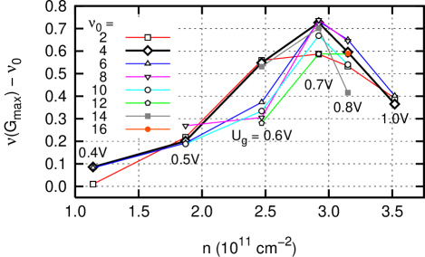
Figure 10: (Color online) Shift of conductance peaks versus electron density. For a fixed base filling factor $\nu_{0}$, the magnetic field rises from the left to the right.

Table 1: Comparison of the filling factor $\nu$ of the second conductance peak (Fig. 6) and the lower ($\varepsilon_{1}$) and upper ($\varepsilon_{2}$) limit of the corresponding gap (Fig. 5(b)) as a result of band structure calculations.

$U_{g}$	$n$ $(10^{11}\ \text{cm}^{-2})$	$B$ $(\text{T})$	$\nu$	$\varepsilon_{1}$	$\varepsilon_{2}$
0.4	1.14	1.15	4.09	2.062	2.072
0.5	1.87	1.84	4.20	2.078	2.091
0.6	2.47	2.25	4.54	2.086	2.100
0.7	2.92	2.56	4.73	2.092	2.107
0.8	3.15	2.84	4.59	2.097	2.113

The position of the conductance peaks in Fig. 6 depends on the electron density. Initially, the peaks shift with increasing density to higher filling factors. For $U_{g}>0.7\ \text{V}$ they shift to lower values again. The displacement of the peak positions with respect to the base filling factor $\nu_{0}=2$, $4$, $6$, $\ldots$ is depicted in Fig. 10, and Table 1 summarizes the properties of the conductance peak $\nu_{0}=4$. All peaks evolve in a very similar way. The decrease of the peak position at high gate voltages can be explainedKang et al. (2000) by the internal bias which is caused by the leakage current trough the barrier. The increase at low electron densities is attributed to the rise of the gap position as shown in Fig. 5(b). One would expect the Fermi energy to jump from one bulk Landau level to another so that non-integer gap positions cannot be realized at all. But as the peaks appear at intermediate values, the Landau bands are assumed to be broadened strongly. Then the relation $\nu=2\left(\varepsilon+\frac{1}{2}\right)$ holds asymptotically for a spin-degenerate system. It allows to compare the band structure with the conductance traces. The numerical calculation yields for the second energy gap a position slightly above the $n=2$ bulk Landau levels (Fig. 5). Starting from spin-degenerate eigenstates, a filling factor of at least $\nu=5.2$ is needed to reach this gap, but the coincidence occurs already at $\nu=4.2\ldots 4.6$. Obviously, the electron-electron interaction between the opposite edge channels is not only responsible for the increased gap, as discussed before, but also for its lowered position. Section II predicts a superlinear increase of the gap position with increasing magnetic field. In detail, the center of the second gap shifts by $\Delta\varepsilon=0.018$ when the field increases from $1.15$ to $1.84\ \text{T}$ as denoted in Table 1. Hence, the corresponding conductance peak is expected to shift by $\Delta\nu=0.036$, whereas the experiment yields $\Delta\nu=0.11$. Another data set, shown in Fig. 8(a), where the magnetic field is slightly shifted due to different experimental conditions, exhibits a rise of $\Delta\nu=0.06$ instead of $2\Delta\varepsilon=0.026$. Consequently, the actual gap position increases on the scale of the cyclotron energy by the factor $2.7\pm 0.4$ stronger than expected from the dispersion calculated in the single electron approximation. This again points towards many body effects which are not included in the calculation.

IV Summary

Our sample structure facilitates the investigation of a certain band gap at different magnetic fields as the Fermi level can be adjusted by means of the gate electrode. Apart from the exploitation of the field effect, the heterostructure differs in the design of the contacts and the barrier from the earlier experiments.Kang et al. (2000); Yang et al. (2004, 2005) Besides the main features of this kind of magneto-tunneling spectroscopy we have especially reproduced at the $\nu_{0}=2$ conductance peak the prominent signature of quantum interferences caused by imperfections in the barrier. At helium-3 temperatures the peak is cropped and shows irregular large-period oscillations. This quenching can be partly suppressed by the internal bias due to gate leakage. Weak AB oscillations are still detectable at $480\ \text{mK}$. In addition, we found very similar quasiperiodic oscillations at low magnetic fields before the onset of the regular conductance peaks. In contrast to the results of Kang, Yang et al., our system is spin-degenerate and the conductance exceeds the limit according to the Landauer-Büttiker formalism. The latter effect is explained by the extended $\text{n}^{+}$-contact layers in conjunction with the separation of the active region into several interrupted quantum Hall systems due to macroscopic defects at the upper $[0\overline{1}0]$-ridge of the sample. Under low gate leakage, measurements at different electron densities reveal a displacement of the conductance peaks towards higher filling factors when the magnetic field is increased. This is in accordance to the single electron band structure which predicts an increase of the gap position on the scale of the cyclotron energy. However, the expected shift is about $1/3$ of $\Delta\nu$ encountered in the experiment.

Two different models have been developed hitherto for the interpretation of this kind of experiment. The picture of Landau level mixingKang et al. (2000); Mitra and Girvin (2001); Kollar and Sachdev (2002); Takagaki and Ploog (2000) estimates the conductance peaks as a consequence of vanishing counterpropagating edge channels when the Fermi level coincides with a gap. For the purpose of investigating the dependence of a certain gap on the magnetic field we have exactly solved the Schrödinger equation in the Landau gauge for a single electron which resides in a 2DES interrupted by a thin tunneling barrier. Parabolic cylinder functions provide a compact representation of the wave functions. The energy dispersion, determined by the continuity at the heterojunctions, has gaps whose positions rise faster than the cyclotron energy when the magnetic field increases. An alternative picture for describing the physics at the junction is based on the coupling of counterpropagating edge states via point contacts in the barrier.Yang et al. (2004, 2005); Kim and Fradkin (2003) The quasiperiodic oscillations at low magnetic field and the properties of the quenched conductance peak can rather be explained within this model.