Electron-beam-induced shift in the apparent position of a pinned vortex in a thin superconducting film

Abstract

When an electron beam strikes a superconducting thin film near a pinned vortex, it locally increases the temperature-dependent London penetration depth and perturbs the circulating supercurrent, thereby distorting the vortex’s magnetic field toward the heated spot. This phenomenon has been used to visualize vortices pinned in SQUIDs using low-temperature scanning electron microscopy. In this paper I develop a quantitative theory to calculate the displacement of the vortex-generated magnetic-flux distribution as a function of the distance of the beam spot from the vortex core. The results are calculated using four different models for the spatial distribution of the thermal power deposited by the electron beam.

I Introduction

An important fundamental property of superfluids and superconductors is that they admit quantized vortices, produced either by rotation of neutral superfluids or by applying magnetic fields to superconductors. Numerous experimental tools have been used to visualize these vortices. In neutral superfluids, charge decoration has been used to observe vortices in superfluid helium,Packard82 and ballistic expansion to observe them in Bose-Einstein condensates.Zwierlein05 In superconducting films, while scanning tunneling microscopyHess89 detects quasiparticles in the vortex core, the localized magnetic-field distributions generated by the circulating supercurrents open the possibility of additional techniques for the observation of singly quantized vortices, such as Bitter decoration,Essmann67 magnetic force microscopy, Moser95 ; Yuan96 scanning SQUID microscopy,Kirtley95 scanning Hall-probe microscopy,Chang92 ; Oral96a ; Oral96b magneto-optical detection,Goa03 Lorentz microscopy,Harada92 and electron holography.Bonevich93 Low-temperature scanning electron microscopy (LTSEM)Clem80 ; Huebener84 ; Bosch85 ; Mannhart87 ; Gross94 ; Doderer97 and laser scanning microscopyScheuermann83 ; Lhota83 have been used to visualize vortices in Josephson junctions.

Recently LTSEM has been used in a new wayStraub01 ; Doenitz04 ; Doenitz06 to detect the presence of pinned vortices in thin-film superconducting quantum interference devices (SQUIDs) at 77 K. When the scanning electron beam strikes the film near a pinned vortex, it locally raises the temperature, decreases the superfluid density, and increases the temperature-dependent London penetration depth $\lambda(T)$. The supercurrent circulating around the vortex is perturbed, the perturbation being a dipole-like backflow current distribution, which generates a corresponding magnetic-field perturbation. As a result, the overall magnetic-field distribution generated by the vortex is no longer centered on the pinned vortex core but is distorted in the direction of the beam spot. The shift in the apparent position of the vortex produces a small change in the return magnetic flux threading the SQUID’s central hole. As the electron beam rasters across the sample, the SQUID output, which is extremely sensitive to such flux changes, can be displayed on a video screen. The resulting image reveals each pinned vortex as a pair of bright and dark spots centered on the vortex, the bright (dark) spot corresponding to an increase (decrease) in the vortex-generated magnetic flux sensed by the SQUID. Since a quantitative description of the above behavior is still lacking, I develop in Sec. II a theory to calculate the displacement of the vortex-generated magnetic-flux distribution as a function of the distance of the beam spot from the vortex core. I present results using four models for the spatial distribution of the thermal power deposited by the electron beam. In Sec. III, I summarize the theoretical results and discuss possible experiments to test the theory.

II Theory

Consider a vortex pinned at the origin in an infinite film of thickness $d$ less than the temperature-dependent London penetration depth $\lambda(T)$, such that the relevant screening length is the Pearl lengthPearl64 $\Lambda(T)=\lambda^{2}/d$. Since the current density $\bm{j}$ is nearly constant across the thickness, we need only consider the sheet-current density $\bm{K}=\bm{j}d$. The magnetic induction generated by the vortex $\bm{B}(\bm{\rho},z)=\nabla\times\bm{A}$ is described by a vector potential $\bm{A}(\bm{\rho},z)$ that in the plane of the film ($z=0$) obeys the London equationLondon61

$$\bm{A}(\bm{\rho},0)+\mu_{0}\Lambda\bm{K}(\bm{\rho})=-\frac{\phi_{0}}{2\pi}\nabla\gamma=\hat{\phi}\frac{\phi_{0}}{2\pi\rho},$$ (1)

where $\bm{K}(\bm{\rho})=(2/\mu_{0})\hat{z}\times\bm{B}(\bm{\rho},0^{+})$, $\phi_{0}=h/2e$ is the superconducting flux quantum, $\gamma$ is the phase of the superconducting order parameter, $\bm{\rho}=x\hat{x}+y\hat{y}$, $\rho=\sqrt{x^{2}+y^{2}}$, $\hat{\rho}=\bm{\rho}/\rho$, and $\hat{\phi}=\hat{z}\times\hat{\rho}$. When the temperature of the film is spatially uniform ($T=T_{0}$), so is the Pearl length $\Lambda=\Lambda(T_{0})=\Lambda_{0}$, and the solution of Eq. (1) is well known. The sheet-current density is Pearl64 ; deGennes66

$$\bm{K}_{0}(\bm{\rho})=\frac{-i\phi_{0}}{2\pi^{2}\mu_{0}}\int\frac{\hat{q}_{\perp}}{1+2q\Lambda_{0}}e^{i\bm{q}\cdot\bm{\rho}}d^{2}q,$$ (2)

where $\bm{q}=q_{x}\hat{x}+q_{y}\hat{y}$, $q=\sqrt{q_{x}^{2}+q_{y}^{2}},$ $\hat{q}=\bm{q}/q$, and $\hat{q}_{\perp}=\hat{z}\times\hat{q}.$ For $\rho\ll\Lambda_{0}$,

$$\bm{K}_{0}(\bm{\rho})\approx\hat{\phi}\phi_{0}/2\pi\mu_{0}\Lambda_{0}\rho,$$ (3)

while for $\rho\gg\Lambda_{0}$,

$$\bm{K}_{0}(\bm{\rho})\approx\hat{\phi}\phi_{0}/\pi\mu_{0}\rho^{2}.$$ (4)

The corresponding magnetic field distribution $\bm{B}_{0}(\bm{\rho},z)$ is centered on the $z$ axis; thus $\int B_{0z}(\bm{\rho},z)d^{2}\rho=\phi_{0}$ and $\int\bm{\rho}B_{0z}(\bm{\rho},z)d^{2}\rho=0$. Above the film at a distance $r=\sqrt{\rho^{2}+z^{2}}$ somewhat greater than $\Lambda_{0}$, $\bm{B}_{0}=\nabla\times\bm{A}_{0}$ appears as if produced by a magnetic monopole at the origin; i.e., $\bm{B}_{0}\approx\hat{r}\phi_{0}/2\pi r^{2}$, where $\bm{r}=\bm{\rho}+z\hat{z}$ and $\hat{r}=\bm{r}/r$.

When a sharply focused electron beam scans across the superconducting film, depositing thermal power $P_{0}$ in the film and its substrate, this locally raises the film’s temperature around the beam spot at $\bm{\rho}_{0}(t)=x_{0}(t)\hat{x}+y_{0}(t)\hat{y}$. As in Refs. Straub01, ; Doenitz04, ; Doenitz06, , I consider slow scans such that the temperature increment quasistatically follows the electron beam and can be written as $\delta T(\bm{\rho}-\bm{\rho}_{0})$. This temperature increment can be calculated by solving the steady-state heat diffusion equation, but this generally requires a detailed knowledge of the initial pear-shaped spatial distribution of the intensity of thermal energy deposition by the e-beam (i.e., the size and shape of the interaction volume), the thermal conductivities $\kappa_{F}$ and $\kappa_{S}$ of the superconducting film and substrate, and the coefficient of heat transfer from the film into the substrate $\alpha_{s}$.Clem80 ; Gross94 In the experiments of Ref. Doenitz06, done at 77 K, the authors estimated that the maximum temperature increment $\Delta T=\delta T(0)$ was only few K. I thus consider only small values of $\Delta T$, such that the deviation of $\Lambda$ from $\Lambda_{0}$, i.e., $\delta\Lambda=\Lambda_{1}(\bm{\rho})=(d\Lambda/dT)\delta T(\bm{\rho})$, is a small perturbation. What is formally needed in the following theory is

$$\delta{\tilde{T}}(\bm{q})=\int\delta T(\bm{\rho})e^{-i\bm{q}\cdot\bm{\rho}}d^{2}\rho,$$ (5)

the two-dimensional Fourier transform of the temperature increment.footnote

To solve for the shift in the apparent position of the pinned vortex when $\Delta T\ll T_{0}$, it is appropriate to use first-order perturbation theory, with $\Lambda=\Lambda_{0}+\Lambda_{1}$ and $\bm{A}(\bm{\rho},z)=A_{0}(\bm{\rho},z)+A_{1}(\bm{\rho},z),$ where quantities with the subscript 1 are proportional to $\Delta T$. Equation (1) yields the boundary condition

$$\bm{A}_{1}(\bm{\rho},0)+\mu_{0}\Lambda_{0}\bm{K}_{1}(\bm{\rho})=-\mu_{0}\Lambda_{1}(\bm{\rho}-\bm{\rho}_{0})\bm{K}_{0}(\bm{\rho}).$$ (6)

It is useful to introduce the Green functions $\bm{a}_{n}(\bm{r})$, $\bm{b}_{n}(\bm{r})=\nabla\times\bm{a}_{n}(\bm{r})$, and $\bm{k}_{n}(\bm{\rho})=(2/\mu_{0})\hat{z}\times\bm{b}_{n}(\bm{\rho},0^{+})$, which obey

$$\bm{a}_{n}(\bm{\rho},0)+\mu_{0}\Lambda_{0}\bm{k}_{n}(\bm{\rho})=-\delta(\bm{\rho})\hat{x}_{n},$$ (7)

where $\hat{x}_{1}=\hat{x},\;\hat{x}_{2}=\hat{y},$ $\bm{r}=(\bm{\rho},z)$, and $n=$ 1 or 2. The solutions are

$$\bm{a}_{n}(\bm{\rho},z)\!\!\! = \!\!\!-\!\!\!\int\!\!\frac{d^{2}q}{(2\pi)^{2}}\{[\hat{q}+i{\rm s}(z)\hat{z}](\hat{q}\cdot\hat{x}_{n})$$ (8)

$$+\frac{\hat{q}_{\perp}(\hat{q}_{\perp}\!\!\cdot\!\hat{x}_{n})}{1+2q\Lambda_{0}}\}e^{i\bm{q}\cdot\bm{\rho}}e^{-q|z|},$$

$$\bm{b}_{n}(\bm{\rho},z)\!\!\! = \!\!\!-\!\!\!\int\!\!\frac{d^{2}q}{(2\pi)^{2}}\frac{q[\hat{q}{\rm s}(z)\!+\!i\hat{z}](\hat{q}_{\perp}\!\!\cdot\!\hat{x}_{n})}{1+2q\Lambda_{0}}e^{i\bm{q}\cdot\bm{\rho}}e^{-q|z|},$$ (9)

$$\bm{k}_{n}(\bm{\rho})\!\!\! = \!\!\!-\frac{2}{\mu_{0}}\!\int\!\!\frac{d^{2}q}{(2\pi)^{2}}\frac{q\hat{q}_{\perp}(\hat{q}_{\perp}\!\!\cdot\!\hat{x}_{n})}{1+2q\Lambda_{0}}e^{i\bm{q}\cdot\bm{\rho}},$$ (10)

where s($z$) = +1 if $z>0$, 0 if $z=0$, and -1 if $z<0$. Then Eq. (6) is solved by

$$\bm{A}_{1}(\bm{\rho},z) = \sum_{n=1}^{2}\int D_{n}(\bm{\rho}^{\prime},\bm{\rho}_{0})\bm{a}_{n}(\bm{\rho}-\bm{\rho}^{\prime},z)d^{2}\rho^{\prime},$$ (11)

$$\bm{B}_{1}(\bm{\rho},z) = \sum_{n=1}^{2}\int D_{n}(\bm{\rho}^{\prime},\bm{\rho}_{0})\bm{b}_{n}(\bm{\rho}-\bm{\rho}^{\prime},z)d^{2}\rho^{\prime},$$ (12)

$$\bm{K}_{1}(\bm{\rho}) = \sum_{n=1}^{2}\int D_{n}(\bm{\rho}^{\prime},\bm{\rho}_{0})\bm{k}_{n}(\bm{\rho}-\bm{\rho}^{\prime})d^{2}\rho^{\prime},$$ (13)

where

$$\bm{D}(\bm{\rho},\bm{\rho}_{0})=\sum_{n=1}^{2}D_{n}(\bm{\rho},\bm{\rho}_{0})\hat{x}_{n}=\mu_{0}\Lambda_{1}(\bm{\rho}-\bm{\rho}_{0})\bm{K}_{0}(\bm{\rho}).$$ (14)

Note that $\nabla\cdot\bm{k}_{n}(\bm{\rho},z)=0$ and $\nabla\cdot\bm{K}_{1}(\bm{\rho},z)=0$ but that $\nabla\cdot\bm{a}_{n}(\bm{\rho},z)\neq 0$ and $\nabla\cdot\bm{A}_{1}(\bm{\rho},z)\neq 0$.

Two important properties of the $z$ component of $\bm{b}_{n}(\bm{\rho},z)$ are that $\int b_{nz}(\bm{\rho},z)d^{2}\rho=0$ and

$$\int\bm{\rho}b_{nz}(\bm{\rho},z)d^{2}\rho=\sum_{m=1}^{2}\delta_{nm}\hat{x}_{m}\times\hat{z}.$$ (15)

Equations (12) and (14) yield $\int B_{1z}(\bm{\rho},z)d^{2}\rho=0$ and

$$\int\bm{\rho}B_{1z}(\bm{\rho},z)d^{2}\rho=\int\bm{D}(\bm{\rho},\bm{\rho}_{0})d^{2}\rho\times\hat{z}.$$ (16)

Using the above properties of $\bm{B}_{0}$ and $\bm{B}_{1}$, we find that to first order in $\Delta T$ the electron-beam-induced shift in the apparent position of the vortex [i.e., the center of the distribution of $B_{z}(\bm{\rho},z)$] is

$$\bm{S}(\bm{\rho}_{0})=\frac{\int\bm{\rho}B_{z}(\bm{\rho},z)d^{2}\rho}{\int B_{z}(\bm{\rho},z)d^{2}\rho}=\frac{1}{\phi_{0}}\int\bm{D}(\bm{\rho},\bm{\rho}_{0})d^{2}\rho\times\hat{z}.$$ (17)

Using Eqs. (2), (5), and (14) and the properties of two-dimensional Fourier transforms, we obtain the following general expression for the shiftfootnote

$$\bm{S}(\bm{\rho}_{0})=\frac{\hat{\rho}_{0}}{\pi}\frac{d\Lambda}{dT}\int_{0}^{\infty}\frac{\delta\tilde{T}(q)}{1+2q\Lambda_{0}}J_{1}(q\rho_{0})qdq$$ (18)

as a function of the beam spot position $\bm{\rho}_{0}=x_{0}\hat{x}+y_{0}\hat{y}$, where $\rho_{0}=\sqrt{x_{0}^{2}+y_{0}^{2}}$, $\hat{\rho}_{0}=\bm{\rho}_{0}/\rho_{0}$, and $J_{n}$ here and in later equations is a Bessel function of the first kind of order $n$. Before we can evaluate the integral in Eq. (18), we need to obtain an expression for $\delta\tilde{T}(q)$ that provides a good description of the experimental conditions.

Let us consider an experimental situation close to that described in Ref. Doenitz06, , in which a well-collimated electron beam of energy $E_{0}=10$ keV, beam current $I_{b}$ = 7 nA, and radius $a\approx$ 5 nm was normally incident upon an epitaxial c-axis-oriented superconducting YBa₂Cu₃O₇ (YBCO) thin film of thickness $d=80$ nm on a thick SrTiO₃ substrate at 77 K. The range $R$, i.e., the maximum distance from the point of incidence the electron travels until it thermalizes, was estimated to be $R\approx$ 0.53 $\mu$m. Each incident electron undergoes numerous elastic and inelastic scattering processes as it loses energy along its diffusion path $s$, and some of this energy emerges from the top surface of the sample as back-scattered electrons, secondary electrons, x-rays, and electromagnetic radiation.Reimer98 The thermal power delivered to the sample is $P_{0}=fI_{b}E_{0}/e$, where the fraction of energy that is ultimately converted into heat is of the order of $f$ = 40-80%.Reimer98

Experiments and Monte Carlo simulations investigating the electron-scattering and energy-loss processes show that the electrons follow relatively straight paths when they are incident upon low-$Z$ targets such as carbon or plastic, such that the diffusion cloud resembles a paint brush.Reimer93 ; Reimer98 On the other hand, when the electrons are incident upon high-$Z$ targets such as gold, the more frequent large-angle elastic scattering processes cause the diffusion cloud to be apple-shaped.Reimer93 ; Reimer98 The highest density of thermal energy deposition is at the center of the beam spot, where all the diffusion paths begin. Because of the complexity of all the electron scattering and diffusion processes, it is not possible to describe the density of thermal power deposition $P_{v}(\rho,z)$ with high accuracy by a simple analytic formula.Reimer98 However, because a mathematical expression for $P_{v}(\rho,z)$ is needed for a calculation of $\delta\tilde{T}(q)$, which appears in the expression for $\bm{S}(\bm{\rho}_{0})$ in Eq. (18), I shall present calculations for four different approximate models. Each model assumes the electron beam is centered on the $z$ axis, $P_{v}(\rho,z)$ is cylindrically symmetric about the $z$ axis, and the volume integral of $P_{v}(\rho,z)$ is equal to $P_{0}$.

First, however, it is useful to consider how to solve for $\delta\tilde{T}(q)$ in general for any given density of thermal power deposition $P_{v}(\rho,z)$. At temperatures in the vicinity of 77 K and above, the temperature perturbation $F(\rho,z)$ in the steady state can be obtained by solving the thermal diffusion equationGross94 $-\kappa\nabla^{2}F=P_{v}$ subject to the boundary condition that $\partial F/\partial z=0$ at the surface $z=0$. This assumes that to good approximation the thermal conductivities of the superconductor and the substrate are the same and equal to $\kappa$. The general solution is

$$F(\rho,z)=\frac{1}{2\pi}\int_{0}^{\infty}\tilde{F}(q,z)J_{0}(q\rho)qdq,$$ (19)

where

$$\tilde{F}(q,z)=\frac{\pi}{\kappa q}\int_{0}^{\infty}d\rho^{\prime}\rho^{\prime}\int_{-\infty}^{0}dz^{\prime}P_{v}(\rho^{\prime},z^{\prime})J_{0}(q\rho^{\prime})$$

$$\times(e^{-q|z-z^{\prime}|}+e^{-q|z+z^{\prime}|}).$$ (20)

The temperature perturbation at the surface is $\delta T(\rho)=F(\rho,0)$ or

$$\delta T(\rho)=\frac{1}{2\pi}\int_{0}^{\infty}\delta\tilde{T}(q)J_{0}(q\rho)qdq,$$ (21)

where

$$\delta\tilde{T}(q)\!=\!\frac{2\pi}{\kappa q}\int_{0}^{\infty}\!\!\!d\rho^{\prime}\rho^{\prime}\!\!\int_{-\infty}^{0}\!\!\!dz^{\prime}P_{v}(\rho^{\prime},z^{\prime})J_{0}(q\rho^{\prime})e^{-q|z^{\prime}|}.$$ (22)

In the limit as $q\rightarrow 0,$ $\delta\tilde{T}(q)$ obeys

$$\delta\tilde{T}(q)\rightarrow\frac{2\pi}{\kappa q}\int_{0}^{\infty}d\rho^{\prime}\rho^{\prime}\int_{-\infty}^{0}dz^{\prime}P_{v}(\rho^{\prime},z^{\prime})=\frac{P_{0}}{\kappa q},$$ (23)

and in the limit as $\rho\rightarrow\infty,$

$$\delta T(\rho)\rightarrow\frac{P_{0}}{2\pi\kappa\rho},$$ (24)

where $P_{0}$ is the total thermal power absorbed by the sample. For each of the models discussed below, the common parameter is $R$, the maximum range of the electron, and it is convenient for later use to express $\delta\tilde{T}(q)$ and $\delta T(\rho)$ in terms of the dimensionless auxiliary functions $h(u)$ and $g(\tilde{\rho})$ via

$$\delta\tilde{T}(q)=\frac{P_{0}}{\kappa q}h(u),$$ (25)

where $u=qR$, and

$$\delta T(\rho)=\frac{P_{0}}{2\pi\kappa R}g(\tilde{\rho}),$$ (26)

where $\tilde{\rho}=\rho/R$,

$$h(u) = u\int_{0}^{\infty}J_{0}(u\tilde{\rho})g(\tilde{\rho})\tilde{\rho}d\tilde{\rho},$$ (27)

$$h(0) = 1,$$ (28)

$$g(\tilde{\rho}) = \int_{0}^{\infty}J_{0}(\tilde{\rho}u)h(u)du,$$ (29)

$$g(0) = \int_{0}^{\infty}h(u)du,$$ (30)

such that

$$\delta T(0)=\frac{P_{0}}{2\pi\kappa R}g(0).$$ (31)

Model KO. To approximate sample heating effects in low-$Z$ materials such as carbon, in which the penetrating electron beam remains relatively straight, Kanaya and OnoKanaya84 introduced a model in which thermal power is deposited with uniform density throughout a cylinder of radius equal to the the beam radius $a$ and length equal to the electron range $R$,

$$P_{v,KO}(\rho,z) = P_{0}/\pi a^{2}R,\rho<a,-R<z<0,$$ (32)

$$= 0,{\rm otherwise}.$$ (33)

The function $h(u)$ defined in Eq. (25) becomes

$$h_{KO}(u)=\frac{J_{1}(\alpha u)}{(\alpha u/2)}\frac{(1-e^{-u})}{u},$$ (34)

where $\alpha=a/R$, and the steady-state temperature increase at the surface is given by Eq. (26), where

$$g_{KO}(\tilde{\rho})=\frac{4}{\pi\alpha^{2}}\int_{0}^{1}d\tilde{z}^{\prime}\int_{0}^{\alpha}d\tilde{\rho}^{\prime}\frac{\tilde{\rho}^{\prime}\bm{K}(k)}{\sqrt{(\tilde{\rho}+\tilde{\rho}^{\prime})^{2}+\tilde{z}^{\prime 2}}},$$ (35)

and $\bm{K}(k)$ is the complete elliptic integral of the first kind of modulus

$$k=\frac{2\sqrt{\tilde{\rho}\tilde{\rho}^{\prime}}}{\sqrt{(\tilde{\rho}+\tilde{\rho}^{\prime})^{2}+\tilde{z}^{\prime 2}}}.$$ (36)

At the center of the beam spot,

$$g_{KO}(0)=\ln\Big{(}\frac{1+\sqrt{1+\alpha^{2}}}{\alpha}\Big{)}+\frac{(\sqrt{1+\alpha^{2}}-1)}{\alpha^{2}}.$$ (37)

Model C. To approximate sample heating effects in higher-$Z$ materials in which the diffusing electron beam spreads out radially from the center of the beam spot into $2\pi$ steradians, one may assume that the thermal power is deposited with the following density,

$$P_{v,C}(r) = P_{0}/2\pi a^{2}R^{\prime},r\leq a,$$ (38)

$$= P_{0}/2\pi r^{2}R^{\prime},a\leq r\leq R,$$ (39)

$$= 0,r\geq R,$$ (40)

where $R^{\prime}=R-2a/3$. This corresponds to the assumption that the maximum density of deposited thermal power occurs at the center of the beam spot but that the diffusing electrons lose energy at a constant rate $-dE/dr$ as they move radially outward, depositing equal amounts of thermal energy into hemispherical shells of increasing volume $2\pi r^{2}dr$ until the electrons thermalize at $r=R$. The function $h(u)$ defined in Eq. (25) becomes

$$h_{C}(u)\!\! =\!\! 1-\frac{1}{(1\!\!-\!\!2\alpha/3)}\{u[J_{0}(u)-(2\alpha^{2}/3)J_{0}(\alpha u)]$$ (41)

$$\!\!-[J_{1}(u)-(2\alpha/3)J_{1}(\alpha u)]-J_{2}(\alpha u)/3u$$

$$\!\!-(\pi u/2)[J_{0}(u)\bm{H}_{1}(u)-J_{1}(u)\bm{H}_{0}(u)]$$

$$\!\!+(\pi u\alpha^{2}/3)[J_{0}(\alpha u)\bm{H}_{1}(\alpha u)-J_{1}(\alpha u)\bm{H}_{0}(\alpha u)]$$

$$\!\!+[J_{0}(u)-J_{0}(\alpha u)]/u\},$$

where $\alpha=a/R$ and $\bm{H}_{n}$ is the Struve function. The steady-state temperature increase at the surface is given by Eq. (26), where

$$g_{C}(\tilde{\rho}) = \frac{1}{(1-2\alpha/3)}\Big{[}\ln\Big{(}\frac{1}{\alpha}\Big{)}+\frac{1}{2}\Big{(}1-\frac{\tilde{\rho}^{2}}{3\alpha^{2}}\Big{)}\Big{]},$$ (43)

$$\;\;\;\;\;\;\;\;\;\;\;\;\;\;\;0\leq\tilde{\rho}\leq\alpha,$$

$$= \frac{1}{(1-2\alpha/3)}\Big{[}\ln\Big{(}\frac{1}{\tilde{\rho}}\Big{)}+\frac{(\tilde{\rho}-2\alpha/3)}{\tilde{\rho}}\Big{]},$$

$$\;\;\;\;\;\;\;\;\;\;\;\;\;\;\;\alpha\leq\tilde{\rho}\leq 1,$$

$$= 1/\tilde{\rho},\;\;\;\;\;\;\;\;\;\;\;\;\tilde{\rho}\geq 1.$$ (44)

At the center of the beam spot,

$$g_{C}(0)=\frac{\ln(1/\alpha)+1/2}{(1\!\!-\!\!2\alpha/3)}.$$ (45)

Model R. Another model, proposed by Reimer,Reimer98 approximates the higher density of power dissipation closer to the beam spot by assuming that the thermal power $P_{0}$ is deposited uniformly within a hemisphere of radius equal to $R/2$,

$$P_{v,R}(r) = \frac{P_{0}}{[2\pi(R/2)^{3}/3]},r<R/2,$$ (46)

$$= 0,r>R/2.$$ (47)

The function $h(u)$ defined in Eq. (25) becomes

$$h_{R}(u)\!\! =\!\! 1-(u/2)J_{0}(u/2)+J_{1}(u/2)+(2/u)J_{2}(u/2)$$

$$\!\!+(\pi u/4)[J_{0}(u/2)\bm{H}_{1}(u/2)-J_{1}(u/2)\bm{H}_{0}(u/2)].$$

The steady-state temperature increase at the surface is given by Eq. (26), where

$$g_{R}(\tilde{\rho}) = 3-4\tilde{\rho}^{2},\;\;0\leq\tilde{\rho}\leq 1/2,$$ (49)

$$= 1/\tilde{\rho},\;\;\;\;\;\;\;\;\;\;\;\;\;\tilde{\rho}\geq 1/2.$$ (50)

At the center of the beam spot,

$$g_{R}(0)=3.$$ (51)

Note that the expression for $h_{R}(u)$ can be obtained from that for $h_{C}(u)$ by setting $\alpha=1$ on the right-hand side of Eq. (41) and then replacing $u=qR$ by $u/2=qR/2$; similarly, the result for $g_{R}(0)$ can be obtained from that for $g_{C}(0)$ by setting $\alpha=1$ on the right-hand side of Eq. (45) and multiplying by a factor of 2.

Model B. A similar model, proposed by Bresse,Bresse72 approximates the density of power dissipation by assuming that the thermal power $P_{0}$ is deposited uniformly within a sphere of radius $R/2$ centered a distance $R/2$ below the surface,

$$P_{v,B}(\rho,z) = \frac{P_{0}}{[4\pi(R/2)^{3}/3]},\sqrt{\rho^{2}+(z+R/2)^{2}}<R/2,$$ (52)

$$-R<z<0,$$

$$= 0,{\rm otherwise}.$$ (53)

The function $h(u)$ defined in Eq. (25) becomes

$$h_{B}(u)=e^{-u/2},$$ (54)

and the steady-state temperature increase at the surface is given by Eq. (26), where

$$g_{B}(\tilde{\rho})=\frac{2}{\sqrt{1+4\tilde{\rho}^{2}}}.$$ (55)

At the center of the beam spot,

$$g_{B}(0)=2.$$ (56)

Figure 1: $h(u)$, the auxiliary function describing the 2D Fourier transform $\delta\tilde{T}(q)$ via Eq. (25), vs $u=qR$ for the four models discussed in the text: KO (dotted), C(solid), R(dashed), and B(dot-dashed) when $\alpha=a/R=0.01$.

Figure 2: $g(\tilde{\rho})$, the auxiliary function describing the temperature perturbation $\delta T(\rho)$ via Eq. (26), vs $\tilde{\rho}=\rho/R$ for the four models discussed in the text: KO (dotted), C(solid), R(dashed), and B(dot-dashed) when $\alpha=a/R=0.01$.

Figures 1 and 2 show plots of the auxiliary functions $h(u)$ vs $u=qR$ and $g(\tilde{\rho})$ vs $\tilde{\rho}=\rho/R$ for the four models KO, C, R, and B in the realistic case that the ratio of the e-beam radius $a$ to the electron range $R$ is $\alpha=a/R=0.01.$

For each of these models, the electron-beam-induced shift in the apparent position of the vortex [see Eqs. (18) and (25)] can be expressed as

$$\bm{S}(\bm{\rho}_{0})=\hat{\rho}_{0}\frac{P_{0}}{\pi\kappa R}\frac{d\Lambda}{dT}G(\rho_{0}/R,2\Lambda_{0}/R),$$ (57)

where $G$ is the dimensionless shift,

$$G(\tilde{\rho}_{0},l)=\int_{0}^{\infty}\frac{h(u)J_{1}(\tilde{\rho}_{0}u)}{1+lu}du,$$ (58)

which is a function of $\tilde{\rho}_{0}=\rho_{0}/R$ and $l=2\Lambda_{0}/R=2\lambda^{2}(T_{0})/Rd$. For models KO and C, $G$ also depends implicitly upon $\alpha=a/R$ [see Eqs. (34) and (41)].

Figure 3: Dimensionless shift $G(\tilde{\rho}_{0},2)$ [Eq. (58)] vs $\tilde{\rho}_{0}=\rho_{0}/R$ for the four models discussed in the text: KO (dotted), C(solid), R(dashed), and B(dot-dashed) when $\alpha=a/R=0.01$ and $l=2\Lambda_{0}/R=2$. As seen in Eq. (57), this function describes the shift in the apparent position of a vortex pinned at the origin when the electron beam strikes the film at a distance $\rho_{0}$ from the origin.

It is straightforward to numerically evaluate the integral in Eq. (58), and Fig. 3 shows plots of $G(\tilde{\rho}_{0},l)$ vs $\tilde{\rho}_{0}=\rho_{0}/R$ for $l=2\Lambda_{0}/R=2$, which is close to the value calculated for the experiments of Ref. Doenitz06, . Although the curves of $G(\tilde{\rho}_{0},l)$ vs $\tilde{\rho}_{0}$ are qualitatively similar, the distinct differences in shapes and maximum slopes may make it possible to determine which of the four models best fits the experimental electron-beam-induced shifts in vortex position. For $\tilde{\rho}_{0}\ll 1,$ the function $G(\tilde{\rho}_{0},l)$ is linear in $\tilde{\rho}_{0}$; i.e., $G(\tilde{\rho}_{0},l)\approx\tilde{\rho}_{0}G^{\prime}(l).$ Since $J_{1}(x)\approx x/2$ for small $x$, the initial slope $G^{\prime}(l)$ can be seen from Eq. (58) to be

$$G^{\prime}(l)=\frac{1}{2}\int_{0}^{\infty}\frac{h(u)u}{1+lu}du.$$ (59)

As shown in Fig. 3, the curves for models KO, C, and R cross near the origin, and for $\alpha=a/R=0.01$ as $\tilde{\rho}_{0}\rightarrow 0,$ the dotted curve (KO) has the steepest slope $G^{\prime}_{KO}(2)=1.25,$ followed by the solid curve (C) with $G^{\prime}_{C}(2)=1.07,$ the dashed curve (R) with $G^{\prime}_{R}(2)=0.53$, and the dot-dashed curve (B) with $G^{\prime}_{B}(2)=0.33$. As expected from the integrands of Eqs. (58) and (59), both $G$ and its initial slope $G^{\prime}$ decrease monotonically with increasing values of $l=2\Lambda_{0}/R$. For large $l$, the initial slope approaches the value $G^{\prime}(l)=g(0)/2l$, and for the four models discussed above, this expression gives, when $\alpha=0.01$, $G^{\prime}_{KO}(l)=2.90/l,$ $G^{\prime}_{C}(l)=2.57/l$, $G^{\prime}_{R}(l)=1.5/l,$ and $G^{\prime}_{B}(l)=1/l$. The largest values of $G$ and $G^{\prime}$ occur for very small values of $l=2\Lambda_{0}/R$. In the limit as $l\rightarrow 0$, the initial slopes are $G^{\prime}_{KO}(0)=(1+\alpha-\sqrt{1+\alpha^{2}})/\alpha^{2}$ or $G^{\prime}_{KO}(0)=99.5$ when $\alpha=0.01$, $G^{\prime}_{C}(0)=(6-3\alpha)/(12\alpha-8\alpha^{2})$ or $G^{\prime}_{C}(0)=50.1$ when $\alpha=0.01$, $G^{\prime}_{R}(0)=3,$ and $G^{\prime}_{B}(0)=2.$

Figure 4 illustrates how the curves of $G(\tilde{\rho}_{0},l)$ vs $\tilde{\rho}_{0}=\rho_{0}/R$ depend upon $l=2\Lambda_{0}/R$ when model KO is used with beam radius $a$ = 5 nm, screening length $\Lambda_{0}$ = 0.5 $\mu$m, but electron range $R$ decreasing (with decreasing beam energy) from $R$ = 100 $\mu$m ($l=0.01$) to $R$ = 0.01 $\mu$m ($l=100$). Similarly, Fig. 5 (note the different scale for the vertical axis) shows how the curves of $G(\tilde{\rho}_{0},l)$ vs $\tilde{\rho}_{0}=\rho_{0}/R$ depend upon $l=2\Lambda_{0}/R$ when model B is used with $\Lambda_{0}$ = 0.5 $\mu$m and $R$ decreasing from $R$ = 100 $\mu$m ($l=0.01$) to $R$ = 0.01 $\mu$m ($l=100$). The general behavior of $G(\tilde{\rho}_{0},l)$ vs $\tilde{\rho}_{0}=\rho_{0}/R$ is very similar for models KO and B, the chief difference being that the slope at the origin is much steeper for model KO than for model B, as discussed above. Corresponding curves for model C would most closely resemble those for model KO, and the curves for model R would most closely resemble those for model B, as can be seen from Fig. 3

Figure 4: Dimensionless shift $G_{KO}(\tilde{\rho}_{0},l)$ vs $\tilde{\rho}_{0}=\rho_{0}/R$, calculated using model KO for fixed $a$ and $\Lambda_{0}$ but decreasing $R$ as described in the text such that $l=2\Lambda_{0}/R$ = 0.01, 0.03, 0.1, 0.3, 1, 3, 10, 30, and 100.

Figure 5: Dimensionless shift $G_{B}(\tilde{\rho}_{0},l)$ vs $\tilde{\rho}_{0}=\rho_{0}/R$, calculated using model B for fixed $\Lambda_{0}$ but decreasing $R$ such that $l=2\Lambda_{0}/R$ = 0.01, 0.03, 0.1, 0.3, 1, 3, 10, 30, and 100.

These results indicate that, for a fixed value of $P_{0}/\pi\kappa R$, the largest shifts in the apparent vortex position [Eq. (57)] occur for values of $l=2\Lambda_{0}/R$ of the order of unity or smaller. The order of magnitude of the shift when $\rho_{0}\sim R$ is then quickly estimated from Eqs. (4), (14), (17), and (31) by noting that $\Lambda_{1}\sim(d\Lambda/dT)\Delta T$ over an area of the order of $\pi R^{2}$ and that $K_{0}(R)\sim\phi_{0}/\pi\mu_{0}R^{2}$, which yields a maximum shift $S(R)\sim(d\Lambda/dT)\Delta T$, where $\Delta T\sim P_{0}/\pi\kappa R$ is the temperature increment at the center of the beam spot. On the other hand, for a fixed electron-beam current $I_{b}$, the maximum shift in the apparent vortex position occurs at an intermediate value of $l$, which can be determined for each of the four models by noting that the prefactor $P_{0}/\pi\kappa R$ depends upon $R=2\Lambda_{0}/l$ not only inversely but also implicitly via the incident electron energy $E_{0}$, as discussed in Sec. III.

III Discussion

In this paper I considered a vortex, pinned at the origin, in a thin film of thickness $d$ when the local heating produced by a scanning electron beam focused at $\bm{\rho}_{0}$ locally raises the film’s temperature, decreases the superfluid density, and increases the London penetration depth $\lambda(T)$. Using first-order perturbation theory, I calculated the resulting vortex-generated supercurrent distribution and the corresponding distortion of the magnetic-field distribution toward the e-beam spot. The resulting expressions for the displacement of the center of the field distribution [Eqs. (57) and (58)] describe how this shift in apparent position depends upon the thermal power $P_{0}$ deposited by the e-beam, the range $R$ over which this power is delivered, the beam radius $a$, the thermal conductivity $\kappa$, the unperturbed screening length (Pearl length) $\Lambda_{0}=\lambda^{2}(T_{0})/d$, the temperature derivative $d\Lambda/dT$ of the screening length, and the distance $\rho_{0}$ between the e-beam spot and the vortex axis.

I calculated the shift $\bm{S}(\bm{\rho}_{0})$ using four different models (KO, C, R, and B) for the spatial dependence of the thermal power deposited by the incident electron beam, all models describing the same total thermal power $P_{0}$ deposited within $R$ of the center of the beam spot. While the results [see Fig. 3] are qualitatively similar for all four models, the detailed functional form of $\bm{S}(\bm{\rho}_{0})$ vs $\bm{\rho}_{0}$ is strongly model-dependent. For example, the slope of $\bm{S}(\bm{\rho}_{0})$ vs $\bm{\rho}_{0}$ at $\bm{\rho}_{0}=0$ is much steeper for models KO and C, which account for the greatly increased density of power deposition near the center of the beam spot, than for models R and B, which assume that the power $P_{0}$ is distributed uniformly over much larger volumes. This suggests that high-resolution experiments, analyzed with the help of the above theory, could be used to determine which of the four models gives the best description of the thermal power density.

To observe e-beam shifts in the apparent position of a pinned vortex, Doenitz et al.Doenitz06 used a SQUID with the central hole in the shape of a long slot. When a vortex was pinned in the body of the SQUID, its return flux was measured by the SQUID with high sensitivity, and any e-beam-induced shift of the vortex’s apparent position toward or away from the slot resulted in a measurable signal, which was displayed as the intensity on a video display as the e-beam was rastered across the sample. Such an image corresponds to a density plot of $S_{x}(x_{0},y_{0})$ vs $x_{0}$ and $y_{0}$. [Note that $S_{x}(-x_{0},y_{0})=-S_{x}(x_{0},y_{0}).$] Shown in Fig. 6 is a density plot of $S_{x}(x_{0},y_{0})$ calculated using model B for the case $l=2\Lambda_{0}/R=2$, roughly equivalent to the experimental conditions of Ref. Doenitz06, , where the authors estimated that $R\approx\Lambda_{0}\approx 0.5\;\mu$m. Figure 6 strongly resembles the vortex images displayed in Ref. Doenitz06, .

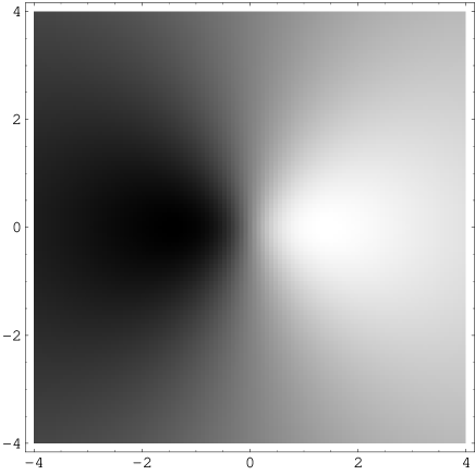
Figure 6: Density plot of the $x$ component of the vortex displacement $S_{x}(x_{0},y_{0})$ vs the electron-beam spot position $(x_{0}/R,y_{0}/R)$ on the superconducting film for the case that $l=2\Lambda_{0}/R=2$, calculated using model B described in the text. Positive values of $S_{x}$ are bright, zero values are grey, and negative values are dark. The vortex, at the center of the plot, shifts to the right (bright areas) when the e-beam strikes to the right of the vortex, and to the left (dark areas) when the e-beam strikes to the left. The maximum displacements are shown as the centers of the bright and dark spots. A horizontal scan through the center of the plot [$S_{x}(x_{0}/R,0)$ vs $x_{0}/R$] corresponds to a plot of $G_{B}(\tilde{\rho}_{0},2)$ vs $\tilde{\rho}_{0}$, as in Fig. 3.

Here is an example of a numerical evaluation of Eq. (57). Assume that the incident electron energy is $E_{0}$ = 10 keV and the beam current is $I_{b}$ = 7 nA, as in Ref. Doenitz06, , and that the fraction of the incident electron energy that is converted into heatReimer98 is $f$ = 0.6, such that $P_{0}$ = 42 $\mu$W. With a SrTiO₃ thermal conductivity $\kappa$ = 18 W/Km at 77 K (Ref. Steigmeier68, ) and an electron range $R$ = 0.53 $\mu$m (Ref. Doenitz06, ), $P_{0}/\pi\kappa R$ = 1.4 K, which is the temperature perturbation at the center of the beam spot according to model B [see Eqs. (26) and (56)]. Assuming $\lambda(T)=(140{\rm\;nm})/\sqrt{1-(T/T_{c})^{4}}$ and film thickness $d$ = 80 nm in $\Lambda=\lambda^{2}(T)/d$, as in Ref. Doenitz06, , one obtains $\Lambda_{0}=\lambda^{2}(T_{0})/d=0.50\;\mu$m and $d\Lambda/dT$ = 27.5 nm/K for YBCO ($T_{c}$ = 91 K) at $T_{0}$ = 77 K, such that $l=2\Lambda_{0}/R$ = 1.9. For model B, the maximum value of $G_{B}(\tilde{\rho}_{0},l)$, which occurs at $\tilde{\rho}_{0}=\rho_{0}/R$ = 1.41, (see Fig. 5) is 0.181, such that the maximum value of $S_{x}(x_{0},y_{0})$ is 7.0 nm at $x_{0}$ = 0.75 $\mu$m and $y_{0}$ = 0. This corresponds to the center of the white spot in Fig. 6. The center of the black spot in Fig. 6 corresponds to the value $S_{x}$ = -7.0 nm at $x_{0}$ = -0.75 $\mu$m and $y_{0}$ = 0.

To test which of the above four models (KO, C, R, or B) is best, similar experiments could be carried out to compare $S_{x}(x_{0},0)$ vs $x_{0}$ for several values of the e-beam radius $a$ for the same incident electron energy and accordingly the same range $R$. According to models KO and C, for the case of an electron range $R$ = 0.53 $\mu$m, as in Ref. Doenitz06, , there should be a significant reduction in the initial slope of $S_{x}(x_{0},0)$ vs $x_{0}$ as the beam radius is varied from $a$ = 5 nm to 50 nm. According to models R and B, however, there should be no significant change in slope.

As another test of the above theory, experiments could be carried out over a wide range of electron energies $E_{0}$ and corresponding electron ranges $R$. Assuming that the range $R\propto E_{0}^{1.43}$, as suggested in Ref. Reimer98, , Doenitz et al.Doenitz06 estimated that $R$ = 0.53 $\mu$m at $E_{0}$ = 10 keV. Assuming that this range-energy relation holds for all energies, one finds the results given in Table I when $\Lambda_{0}$ = 0.50 $\mu$m. Comparisons of experimental results with theoretical plots of $S_{x}(x_{0},0)$ vs $x_{0}$ obtained from calculations such as those shown in Figs. 4 and 5 would provide a stringent test of the four models.

Table 1: Calculated values of $l=2\Lambda_{0}/R$, electron range $R=$ 0.53 $\mu$m$(E_{0}$/10 keV$)^{1.43}$, and electron-beam energy $E_{0}$ when $\Lambda_{0}=0.50$ $\mu$m.

$l$	$R$ ($\mu$m)	$E_{0}$ (keV)
0.01	100	390
0.03	33	181
0.1	10	78
0.3	3.3	36
1	1	16
3	0.33	7.2
10	0.1	3.1
30	0.033	1.4
100	0.01	0.62

Experiments done at various temperatures above 77 K would provide a further test of the theory. In Ref. Doenitz06, , Doenitz et al. estimated the value of $\Lambda_{0}=\lambda^{2}(T_{0})/d\approx 0.50\;\mu$m for YBCO ($T_{c}$ = 91 K) of thickness 80 nm at $T_{0}$ = 77 K by assuming $\lambda(T)=(140{\rm\;nm})/\sqrt{1-(T/T_{c})^{4}}$. With $R$ = 0.53 $\mu$m, this gives a value of $l=2\Lambda_{0}/R=1.9$. Increasing the temperature would not only increase the value of $l$ and decrease the magnitude of $G$ (see Figs. 4 and 5) but also increase the magnitude of $d\Lambda/dT$. For large $l$, the combination of these two competing effects would lead to an overall increase in the magnitude of $S_{x}(x_{0},y_{0})\propto(1/\Lambda_{0})(d\Lambda/dT)$ according to Eqs. (57) and (58). With the temperature $T$ approaching $T_{c}$, however, it is likely that the vortex would become depinned and follow the warmer beam spot, such that the above theory, which assumes that the vortex remains pinned as the electron beam scans over it, would no longer apply.

Reducing the temperature to lower values would decrease the value of $l$, thereby increasing the magnitude of $G$. On the other hand, it is likely that the reduced value of $d\Lambda/dT$ would more than compensate for this effect and lead to an overall decrease in the magnitude of $S_{x}(x_{0},y_{0})$. Going to low temperatures, however, would put the experiments in a temperature range where the above theory for the temperature increment involving only the thermal conductivity $\kappa$ is no longer valid.Gross94

It is important to note that the above theory is expected to be valid for experiments on superconducting films at liquid-nitrogen temperatures or above. At much lower temperatures, including liquid-helium temperatures, the above calculations of the temperature perturbation [Eqs. (19)-(31)] are no longer valid, because it is then essential to take into account the thermal boundary resistance between the superconducting film and the substrate.Clem80 ; Huebener84 ; Gross94 In such a case, the theory involves an additional length scale, $\eta=(\kappa d/\alpha_{s})^{1/2}$, the thermal healing length, where $\alpha_{s}$ is the coefficient of heat transfer from the superconducting film into the substrate.Clem80 ; Huebener84 ; Gross94

Although the results given in this paper apply strictly only to a vortex in an infinite thin film, I expect that when $R\geq\Lambda_{0}$, Eqs. (57) and (58) also apply to good approximation to a vortex in a thin film with finite lateral dimensions, provided that the distance of the vortex from the edge of the film is more than a few $R$. This is because the current-density perturbation is largest within an area of order $R^{2}$ when the electron beam is roughly a distance $R$ from the vortex. However, when the distance of the vortex from the edge of the film is approximately $R$ or smaller, the above calculation would have to be redone, taking into account how the supercurrent is modified near the film edge.

- (1) R. E. Packard, Physica B+C 109-110, 1474 (1982).
- (2) M. W. Zwierlein, J. R. Abo-Shaeer, A. Schirotzek, C. H. Schunck, and W. Ketterle, Nature 435, 1047 (2005).
- (3) H. F. Hess, R. B. Robinson, R. C. Dynes, J. M. Valles, Jr., and J. V. Waszczak, Phys. Rev. Lett. 62, 214 (1989).
- (4) U. Essmann and H. Träuble, Phys. Lett. 24A, 526 (1967); H. Träuble and U. Essmann, Phys. Stat. Sol. 95, 373 and 395 (1968).
- (5) A. Moser, H. J. Hug, I. Parashikov, B. Stiefel, O. Fritz, H. Thomas, A. Baratoff, H.-J. Gu ntherodt, and P. Chaudhari, Phys. Rev. Lett. 74, 1847 (1995).
- (6) C. W. Yuan, Z. Zheng, A. L. de Lozanne, M. Tortonese, D. A. Rudman, and J. N. Eckstein, J. Vac. Sci. Technol. B 14, 1210 (1996).
- (7) J. R. Kirtley, M. B. Ketchen, K. G. Stawlasz, J. Z. Sun, W. J. Gallagher, S. H. Blanton, and S. J. Wind, Appl. Phys. Lett. 66, 1138 (1995).
- (8) A. M. Chang, H. D. Hallen, L. Harriott, H. F. Hess, H. L. Kao, J. Kwo, R. E. Miller, R. Wolfe, J. van der Ziel, and T. Y. Chang Appl. Phys. Lett. bf 61, 1974 (1992).
- (9) A. Oral, S. J. Bending, and M. Henini, J. Vac. Sci. Technol. B 14, 1202 (1996).
- (10) A. Oral, S. J. Bending, and M. Henini, Appl. Phys. Lett. 69, 1324 (1996).
- (11) P. F. Goa, H. Hauglin, Å. A. F. Olsen, M. Baziljevich, and T. H. Johansen, Rev. Sci. Instrum. 74, 141 (2003).
- (12) K. Harada, T. Matsuda, J. Bonevich, M. Igarashi, S. Kondo, G. Pozzi, U. Kawabe, and A. Tonomura, Nature 360, 51 (1992).
- (13) J. E. Bonevich, K. Harada, T. Matsuda, H. Kasai, T. Yoshida, G. Pozzi, and A. Tonomura, Phys. Rev. Lett. 70, 2952 (1993).
- (14) J. R. Clem and R. P. Huebener, J. Appl. Phys. 51, 2764 (1980).
- (15) R. P. Huebener, Rep. Prog. Phys. 47, 175 (1984).
- (16) J. Bosch, R. Gross, M. Koyanagi, and R. P. Huebener, Phys. Rev. Lett. 54, 1448 (1983).
- (17) J. Mannhart, J. Bosch, R. Gross, and R. P. Huebener, Phys. Rev. B35, 5267 (1987).
- (18) R. Gross and D. Koelle, Rep. Prog. Phys. 57, 651 (1994).
- (19) T. Doderer, Int. J. Mod. Phys. B 11, 1979 (1997).
- (20) M. Scheuermann, J. R. Lhota, P. K. Kuo, and J. T. Chen, Phys. Rev. Lett. 50, 74 (1983).
- (21) J. R. Lhota, M. Scheuermann, P. K. Kuo, and J. T. Chen, Appl. Phys. Lett. 44, 255 (1983).
- (22) R. Straub, S. Keil, R. Kleiner, and D. Koelle, Appl. Phys. Lett. 78, 3645 (2001).
- (23) D. Doenitz, R. Straub, R. Kleiner, and D. Koelle, Appl. Phys. Lett. 85, 5938 (2004).
- (24) D. Doenitz, M. Ruoff, E. H. Brandt, J. R. Clem, R. Kleiner, and D. Koelle, Phys. Rev. B73, 064508 (2006).
- (25) J. Pearl, Appl. Phys. Lett. 5, 65 (1964).
- (26) F. London, Superfluids, Vol. 1 (Dover, New York, 1961).
- (27) P. G. de Gennes, Superconductivity of Metals and Alloys (Benjamin, New York, 1966)
- (28) I assume here that depends only upon , such that depends only upon .
- (29) L. Reimer, Scanning Electron Microscopy, 2nd ed. (Springer, Berlin, 1998).
- (30) L. Reimer, Image Formation in Low-Voltage Scanning Electron Microscopy (SPIE Optical Engineering Press, Bellingham, 1993).
- (31) K. Kanaya and S. Ono, in Electron Beam Interactions with Solids for Microscopy, Microanalysis, and Microlithography, edited by D. F. Kyser, H. Niedrig, D. E. Newbury, and R. Shimizu (Scanning Electron Microscopy, AMF O’Hare, 1984), p. 69.
- (32) J. F. Bresse, in Scanning Electron Microscopy 1972, edited by O. Johari and I. Corvin (IITRI, Chicago, 1972), p. 105.
- (33) E. F. Steigmeier, Phys. Rev. 168, 523 (1968).