Correlation functions of a Lieb-Liniger Bose gas

Abstract

The ground-state correlation functions of a one-dimensional homogeneous Bose system described by the Lieb-Liniger Hamiltonian are investigated by using exact quantum Monte Carlo techniques. This article is an extension of a previous study published in Phys. Rev. A 68, 031602 (2003). New results on the local three-body correlator as a function of the interaction strength are included and compared with the measured value from three-body loss experiments. We also carry out a thorough study of the short- and long-range behavior of the one-body density matrix.

I Introduction

Recent progress achieved in techniques of confining Bose condensates has lead to experimental realizations of quasi-one-dimensional (1D) systemsMIT ; Paris ; Zurich ; Laburthe Tolra ; Paredes ; PennStateU . The quasi-1D regime is reached in highly anisotropic traps, where the axial motion of the atoms is weakly confined while the radial motion is frozen to zero point oscillations by the tight transverse trapping. These experimental achievements have revived interest in the theoretical study of the properties of 1D Bose gases. In most applications, a single parameter, the effective 1D scattering length $a_{1D}$, is sufficient to describe the interatomic potential, which in this case can be conveniently modeled by a $\delta$-function pseudopotential. For repulsive effective interactions the relevant model is provided by the Lieb-Liniger Hamiltonian LL1 . Many properties of this integrable model such as the ground-state energy LL1 , the excitation spectrum LL2 and the thermodynamic functions at finite temperature YY were obtained exactly in the 60’ using the Bethe ansatz method. Less is known about correlation functions, for which analytic results were obtained only in the strongly interacting regime of impenetrable bosons Corr tonks and for the long-range behavior of the one-body density matrix Schwartz . More recently, the properties of correlation functions of the Lieb-Liniger model have attracted considerable attention and the short-range expansion of the one-body density matrix Olshanii , as well as the local two- and three-body correlation function Gangardt have been investigated. However, a precise determination of the spatial variation of correlation functions for arbitrary interaction strength is lacking.

We use exact quantum Monte Carlo methods to investigate the behavior of correlation functions in the ground state of the Lieb-Liniger model. Over a wide range of values for the interaction strength, we calculate the one- and two-body correlation function and their Fourier transform giving, respectively, the momentum distribution and the static structure factor of the system. These results were already presented in a previous study (Ref. us ) and are briefly reviewed here. We present new results on the local three-body correlation function ranging from the weakly- up to the strongly-interacting regime. We have also investigated in more details the long- and short-range behavior of the one-body density matrix, including a discussion of finite-size effects and of the validity of the trial function used for importance sampling. We always provide quantitative comparisons with known analytical results obtained in the weak- or strong-correlation regime, or holding at short or large distances. In the case of the local three-body correlator we also compare with available experimental results obtained from three-body loss measurements Laburthe Tolra .

The structure of the paper is as follows. In section II we introduce the definitions of the spatial correlation functions and their Fourier transform. In section III we discuss the Lieb-Liniger model and give a summary of the main known results concerning correlation functions in this model. Section IV is devoted to a brief description of the quantum Monte Carlo method used for the numerical solution of the Schrödinger equation. The optimization of the trial wave function used for importance sampling and the effects due to finite-size are discussed here. The results for correlation functions are presented in section V. Finally, in section VI we draw our conclusions.

II Correlation functions

We use the first quantization definition of correlation functions in terms of the many-body wave function of the system $\Psi(z_{1},...,z_{N})$, where $z_{1},...,z_{N}$ denote the coordinates of the $N$ particles. We are interested in the regime where the most relevant fluctuations are of quantum nature. In the following we will always consider homogeneous systems at $T=0$ and the ground-state wave function of the system will be denoted by $\Psi_{0}(z_{1},...,z_{N})$.

The one-body density matrix $g_{1}(z)$ describes the spatial correlations in the wave function and is defined as

$$g_{1}(z)=\frac{N}{n}\frac{\int\Psi_{0}^{*}(z_{1}+z,...,z_{N})\Psi_{0}(z_{1},...,z_{N})\,dz_{2}...dz_{N}}{\int|\Psi_{0}(z_{1},...,z_{N})|^{2}\,dz_{1}...dz_{N}}\;,$$ (1)

where $n=N/L$ is the one-dimensional density. The normalization of $g_{1}(z)$ is chosen in such a way that $g_{1}(0)=1$.

Another important quantity is the pair distribution function $g_{2}(|z_{1}-z_{2}|)$, which corresponds to the probability of finding two particles separated by $|z_{1}-z_{2}|$:

$$g_{2}(|z_{1}-z_{2}|)=\frac{N(N-1)}{n^{2}}\frac{\int|\Psi_{0}(z_{1},...,z_{N})|^{2}\,dz_{3}...dz_{N}}{\int|\Psi_{0}(z_{1},...,z_{N})|^{2}\,dz_{1}...dz_{N}}\;.$$ (2)

The normalization is chosen in such a way that at large distances $g_{2}(z)$ goes to $1-\frac{1}{N}$, i.e. becomes unity in the thermodynamic limit $N\to\infty$.

The value at zero distance of the three-body correlation function gives the probability of finding three particles at the same position in space

$$g_{3}(0)=\frac{N(N-1)(N-2)}{n^{3}}\frac{\int|\Psi_{0}(0,0,0,z_{4},...,z_{N})|^{2}\,dz_{4}...dz_{N}}{\int|\Psi_{0}(z_{1},...,z_{N})|^{2}\,dz_{1}...dz_{N}}\;.$$ (3)

The knowledge of the density dependence of $g_{3}(0)$ allows one to estimate the rate of three-body recombinations which is of great experimental relevance Laburthe Tolra .

Much useful information can be obtained from the Fourier transform of the above correlation functions. The momentum distribution $n(k)$ is related to the one-body density matrix [Eq. (1)]:

$$n(k)=n\int e^{ikz}g_{1}(z)\,dz\;,$$ (4)

and the static structure factor $S(k)$ is instead related to the pair distribution function [Eq. (2)]:

$$S(k)=1+n\int e^{ikz}(g_{2}(z)-1)\,dz\;.$$ (5)

The momentum distribution can be measured in time of flight experiments Paredes and the static structure factor using Bragg spectroscopy BraggSpectroscopy .

III Lieb-Liniger Hamiltonian

A bosonic gas at $T=0$, confined in a waveguide or in a very elongated harmonic trap, can be described in terms of a one-dimensional model if the energy of the motion in the longitudinal direction is insufficient to excite the levels of the transverse confinement. Further, if the range of the interatomic potential is much smaller than the interparticle distance and the characteristic length of the external confinement, a single parameter is sufficient to describe interactions, namely the effective one-dimensional scattering length $a_{1D}$. In this case the particle-particle interactions can be safely modeled by a $\delta$-pseudopotential. Such a system is described by the Lieb-Liniger (LL) Hamiltonian LL1 :

$$\hat{H}_{LL}=-\frac{\hbar^{2}}{2m}\sum\limits_{i=1}^{N}\frac{\partial^{2}}{\partial z^{2}_{i}}+g_{1D}\sum\limits_{i<j}\delta(z_{i}-z_{j})\;,$$ (6)

where the coupling constant $g_{1D}$ is related to $a_{1D}$ by $g_{1D}=-2\hbar^{2}/ma_{1D}$, $m$ being the particle mass. In the presence of a tight harmonic transverse confinement, characterized by the oscillator length $a_{\perp}=\sqrt{\hbar/m\omega_{\perp}}$, the scattering length $a_{1D}$ was shown to exhibit a non trivial behavior in terms of the 3D $s$-wave scattering length $a_{3D}$ due to virtual excitations of transverse oscillator levels Olshanii g1D

$$a_{1D}=-a_{\perp}\left(\frac{a_{\perp}}{a_{3D}}-1.0326\right)\;.$$ (7)

In typical experimental conditions, far from a Feshbach resonance, one has $a_{3D}\ll a_{\perp}$. In this case the above equation simplifies to $a_{1D}=-a_{\perp}^{2}/a_{3D}$, which coincides with the mean-field prediction Petrov . In the vicinity of a magnetic Feshbach resonance the value of $a_{3D}$ can become comparable with $a_{\perp}$ and the coupling constant $g_{1D}$ varies over a wide range as it goes through a confinement induced resonance Olshanii g1D .

All properties in the model depend only on one parameter, the dimensionless density $n|a_{1D}|$. Contrary to the 3D case, where at low density the gas is weakly interacting, in 1D small values of the gas parameter $n|a_{1D}|$ correspond to strongly correlated systems. This peculiarity of 1D systems can be easily understood by comparing the characteristic kinetic energy $\hbar^{2}n^{2/D}/2m$, where $D$ denotes the dimensionality, to the mean-field interaction energy $gn$. In 3D, $g_{3D}n\propto n|a_{3D}|\ll n^{2/3}$ if $n|a_{3D}|^{3}\ll 1$. In 1D, instead, $g_{1D}n\propto n/|a_{1D}|\gg n^{2}$ if $n|a_{1D}|\ll 1$.

The ground-state energy of the Hamiltonian (6) with $g_{1D}>0$ was first obtained by Lieb and Liniger LL1 using the Bethe ansatz method. The energy of the system is conveniently expressed as $E/N=e(n|a_{1D}|)\hbar^{2}n^{2}/2m$, where the function $e(n|a_{1D}|)$ is obtained by solving a system of integral equations. In the mean-field Gross-Pitaevskii (GP) regime, $n|a_{1D}|\gg 1$, the energy per particle is linear in the density $E^{GP}/N=g_{1D}n/2$, while in the strongly correlated Tonks-Girardeau (TG) regime, $n|a_{1D}|\ll 1$, the dependence is quadratic $E^{TG}/N=\pi^{2}\hbar^{2}n^{2}/6m$. The equation of state resulting from a numerical solution of the LL integral equations is shown in Fig. 1 as a function of the gas parameter $n|a_{1D}|$.

Figure 1: Energy per particle: Bethe ansatz solution (solid line); GP limit (dashed line); TG limit (dotted line). The circles are the results of DMC calculations. Energies are in units of $\hbar^{2}/(ma_{1D}^{2})$.

In the TG regime, the energy of an incident particle is not sufficient to tunnel through the repulsive interaction potential and two particles will never be at the same position in space. This constraint, together with the spatial peculiarity of 1D systems, acts as an effective Fermi exclusion principle. Indeed, in this limit, the system of bosons acquires many Fermi-like properties. There exists a direct mapping of the wave function of strongly interacting bosons onto a wave function of non interacting spinless fermions due to Girardeau Girardeau . The chemical potential, $\mu=\partial E/\partial N$, of a TG gas equals the 1D Fermi energy $\mu=\hbar^{2}k_{F}^{2}/2m$, where $k_{F}=\pi n$ is the Fermi wave vector, and the speed of sound $c$, defined through the inverse compressibility $mc^{2}=n\partial\mu/\partial n$, is given by $c=\hbar k_{F}/m$.

Further, the pair distribution function

$$g_{2}(z)=1-\frac{\sin^{2}\pi nz}{(\pi nz)^{2}}\;,$$ (8)

which exhibits Friedel-like oscillations, and the static structure factor of the TG gas

$$S(k)=\left\{\begin{array}[]{cc}|k|/(2\pi n),&|k|<2\pi n\\ 1,&|k|>2\pi n\;,\\ \end{array}\right.$$ (9)

can be calculated exactly exploiting the Bose-Fermi mapping Girardeau .

The one-body density matrix $g_{1}(z)$ of a TG gas has been calculated in terms of series expansions holding at small and large distances in Ref. Corr tonks . The leading long-range term decays as

$$g_{1}(z)=\frac{\sqrt{\pi e}2^{-1/3}A^{-6}}{\sqrt{|z|n}}\;,$$ (10)

($A=1.28...$ is Glaisher’s constant) and yields an infrared divergence in the momentum distribution $n(k)\propto 1/\sqrt{|k|/n}$.

Outside the TG regime full expressions of the correlation functions are not known. The long-range asymptotics can be calculated using the hydrodynamic theory of the low-energy phonon-like excitations Reatto ; Schwartz ; Korepin . For $g_{1}(z)$ one finds the power-law decay

$$g_{1}(z)=\frac{C_{asympt}}{|zn|^{\alpha}}\;,$$ (11)

where $\alpha=mc/(2\pi\hbar n)$ and $C_{asympt}$ is a numerical coefficient. This result holds for distances $|z|\gg\xi$, where $\xi=\hbar/(\sqrt{2}mc)$ is the healing length. In the TG regime $c=\pi\hbar n/m$ and $\alpha=1/2$ as anticipated above. In the opposite GP regime ($n|a_{1D}|\gg 1$) one finds $\alpha=1/(\pi\sqrt{2n|a_{1D}|})$, yielding a vanishingly small value for $\alpha$. The power-law decay of the one-body density matrix excludes the existence of Bose-Einstein condensation in infinite systems Schultz . The behavior of the momentum distribution for $|k|\ll 1/\xi$ follows immediately from Eq. (11):

$$n(k)=C_{asympt}\left|\frac{2n}{k}\right|^{1-\alpha}\frac{\sqrt{\pi}\Gamma\left(\frac{1}{2}-\frac{\alpha}{2}\right)}{\Gamma\left(\frac{\alpha}{2}\right)}\;,$$ (12)

where $\Gamma(z)$ is the Gamma function.

The hydrodynamic theory allows one to calculate also the static structure factor in the long-wavelength regime, $|k|\ll 1/\xi$. One finds the well-known Feynmann result Feynmann

$$S(k)=\frac{\hbar|k|}{2mc}\;.$$ (13)

Recently, the short-range behavior of the one-, two-, and three-body correlation functions has also been investigated. The value at $z=0$ of the pair correlation function for arbitrary densities can be obtained from the equation of state through the Hellmann-Feynman theorem Gangardt :

$$g_{2}(0)=-\frac{(n|a_{1D}|)^{2}}{2}e^{\prime}\;,$$ (14)

where the derivative of the equation of state $e(n|a_{1D}|)$ is to be taken with respect to $n|a_{1D}|$.

The $z=0$ value of the three-body correlation function was obtained within a perturbation scheme in the regions of strong and weak interactions Gangardt . It is very small in the TG limit ($n|a_{1D}|\ll 1$)

$$g_{3}(0)=\frac{(\pi n|a_{1D}|)^{6}}{60}\;,$$ (15)

and goes to unity in the GP regime ($n|a_{1D}|\gg 1$)

$$g_{3}(0)=1-\frac{6\sqrt{2}}{\pi\sqrt{n|a_{1D}|}}\;.$$ (16)

The first terms of the short-range expansion of $g_{1}(z)$ can also be calculated from the knowledge of the equation of state Olshanii

$$g_{1}(z)=1-\frac{1}{2}(e+e^{\prime}n|a_{1D}|)(nz)^{2}+\frac{e^{\prime}}{6}(n|z|^{3})\;,$$ (17)

holding for arbitrary densities and for small distances $n|z|\ll 1$.

IV Quantum Monte Carlo Method

We use Variational Monte Carlo (VMC) and Diffusion Monte Carlo (DMC) methods in order to study the ground-state properties of the system. In VMC one calculates the expectation value of the Hamiltonian over a trial wave function $\psi_{T}({\bf R},A,B,...)$, where ${\bf R}=(z_{1},...,z_{N})$ denotes the particle coordinates and $A$, $B$, … are variational parameters. According to the variational principle, the energy

$$E_{VMC}=\frac{\langle\psi_{T}|\hat{H}|\psi_{T}\rangle}{\langle\psi_{T}|\psi_{T}\rangle}$$ (18)

provides an upper bound to the ground-state energy, $E_{VMC}\geq E_{0}$. The variational parameters $A,B,...$ are optimized by minimization of the variational energy (18).

In order to remove the bias in the estimate of the ground-state energy caused by the particular choice of the trial wave function, we resort to the DMC method, which allows one to solve exactly, apart from statistical uncertainty, the many-body Schrödinger equation of a Bose system at zero temperature BORO1 . The evolution in imaginary time, $\tau=it/\hbar$, is performed for the product $f({\bf R},\tau)=\psi_{T}({\bf R})\Psi({\bf R},\tau)$, where $\Psi({\bf R},\tau)$ denotes the wave function of the system and $\psi_{T}({\bf R})$ is a trial function used for importance sampling. The time-dependent Schrödinger equation for the function $f({\bf R},\tau)$ can be written as

$$-\frac{\partial f({\bf R},\tau)}{\partial\tau}= - D\nabla_{\bf R}^{2}f({\bf R},\tau)+D\nabla_{\bf R}[{\bf F}({\bf R})f({\bf R},\tau)]+[E_{L}({\bf R})-E_{ref}]f({\bf R},\tau)\;,$$ (19)

where $E_{L}({\bf R})=\psi_{T}({\bf R})^{-1}H\psi_{T}({\bf R})$ denotes the local energy, ${\bf F}({\bf R})=2\psi_{T}({\bf R})^{-1}\nabla_{\bf R}\psi_{T}({\bf R})$ is the quantum drift force, $D=\hbar^{2}/(2m)$ plays the role of an effective diffusion constant, and $E_{ref}$ is a reference energy introduced to stabilize the numerical evaluation. The energy and other observables of the state of the system are calculated from averages over the asymtpotic distribution function $f({\bf R},\tau\to\infty)$. It is easy to check by decomposing $f({\bf R},\tau)$ on the basis of stationary states of the Hamiltonian, that contributions of the excited states vanish exponentially fast with the imaginary time $\tau$ and asymptotically one obtains $\lim_{\tau\to\infty}f({\bf R},\tau)=\psi_{T}({\bf R})\Psi_{0}({\bf R})$ for all trial wave functions non orthogonal to the ground-state wave function $\Psi_{0}({\bf R})$. The local energy $E_{L}$ sampled over the asymptotic distribution equals exactly the ground-state energy

$$\lim_{\tau\to\infty}\frac{\int E_{L}({\bf R})f({\bf R},\tau)\,d{\bf R}}{\int f({\bf R},\tau)\,d{\bf R}}=\frac{\langle\psi_{T}|\hat{H}|\Psi_{0}\rangle}{\langle\psi_{T}|\Psi_{0}\rangle}=E_{0}\;.$$ (20)

In the present study the trial wave function is chosen of the the Bijl-Jastrow form:

$$\psi_{T}(z_{1},...,z_{N})=\prod_{i<j}f(z_{ij}),$$ (21)

where $f(z)$ is a two-body term chosen as

$$f(z)=\left\{\begin{array}[]{lr}A\cos[k(|z|-B)],&|z|<Z\\ \sin^{\beta}(\pi|z|/L),&|z|>Z\;.\\ \end{array}\right.$$ (22)

We consider $N$ particles in a box of size $L$ with periodic boundary conditions. In the construction of the trial wave function we have ensured that $f(z)$ is uncorrelated at the box boundaries, $f(z=\pm L/2)=1$ and the derivative $f^{\prime}(z=\pm L/2)=0$. For $|z|<Z$, the Bijl-Jastrow term $f(z)$ corresponds to the exact solution of the two-body problem with the potential $g_{1D}\delta(z)$ and provides a correct description of short-range correlations. Long-range correlations arising from phonon excitations are instead accounted for by the functional dependence of $f(z)$ for $|z|>Z$ Reatto . The $z=0$ boundary condition $f^{\prime}(0^{+})-f^{\prime}(0^{-})=2f(0)/|a_{1D}|$, which accounts for the $\delta$-function potential, fixes the parameter $k$ through the relation $k|a_{1D}|\tan kB=1$. The remaining parameters $A,B$ and $\beta$ are fixed by the continuity conditions at the matching point $z=Z$ of the function $f(z)$, its derivative $f^{\prime}(z)$ and the local energy $-2f^{\prime\prime}(z)/f(z)$. The value of the matching point $Z$ is a variational parameter which we optimize using VMC. The TG wave function of Ref. Girardeau , $\Psi_{0}^{TG}=\prod_{i<j}|\sin[\pi(z_{i}-z_{j})/L]|$, is obtained as a special case of our trial wave function $\psi_{T}$ for $Z=B=L/2$ and $kL=\pi$.

The choice of a good trial wave-function is crucial for the efficiency of the calculation. In order to prove that our trial wave-function is indeed very close to the true ground-state $\Psi_{0}({\bf R})$, we compare in Table I the variational energy $E_{VMC}$ with the exact solution based on the use of the Bethe ansatz LL1 . The corresponding results obtained using DMC coincide, within statistical uncertainty, with the exact ones and are shown in Fig. 1.

$n|a_{1D}|$	$E_{LL}/N$	$E_{VMC}/N$
$10^{-3}$	$1.6408\cdot 10^{-6}$	$1.6415(1)\cdot 10^{-6}$
$0.03$	$1.3949\cdot 10^{-3}$	$1.3957(3)\cdot 10^{-3}$
$0.3$	$9.0595\cdot 10^{-2}$	$9.093(1)\cdot 10^{-2}$
$1$	$0.5252$	$0.5259(1)$
$30$	$26.842$	$27.19(5)$
$10^{3}$	$981.15$	$983.6(3)$

Table 1: Energy per particle for different values of the gas parameter $n|a_{1D}|$: $E_{LL}$ — exact result obtained by solving the Lieb-Liniger equations, $E_{VMC}$ — variational result, Eq. (18), obtained from optimization of the trial wave function (22).

Besides the ground-state energy $E_{0}$, the DMC method gives exact results also for local correlation functions, such as the pair distribution function $g_{2}(z)$ and the three-body correlator $g_{3}(0)$, for which one can use the method of “pure” estimators BORO2 . Instead, in the calculation of the non-local one-body density matrix $g_{1}(z)$, the bias from the trial wave function can be reduced using the extrapolation technique: $\langle\Psi_{0}|\hat{A}|\Psi_{0}\rangle=2\,\langle\Psi_{0}|\hat{A}|\psi_{T}\rangle-\langle\psi_{T}|\hat{A}|\psi_{T}\rangle$, written here for a generic operator $\hat{A}$. The “mixed” estimator $\langle\Psi_{0}|\hat{A}|\psi_{T}\rangle$ is the direct output of the DMC calculation and the variational estimator $\langle\psi_{T}|\hat{A}|\psi_{T}\rangle$ is obtained from a VMC calculation. This procedure is accurate only if $\psi_{T}\simeq\Psi_{0}$. In the present study DMC and VMC give results for $g_{1}(z)$ which are very close and we believe that the extrapolation technique removes completely the bias from $\Psi_{T}({\bf R})$.

Calculations are carried out for a finite number of particles $N$. In order to extrapolate to infinite systems, we increase $N$ and study the convergence in the quantities of interest. The dependence on the number of particles (so called finite-size effect) is more pronounced in the regime $n|a_{1D}|\gg 1$, where correlations extend to very large distances. Finite size effects can be best investigated by considering the one-body density matrix. In Fig. 2 we show $g_{1}(z)$ at a fixed density, $n|a_{1D}|=30$, for systems of $N=50,100,200,500$ particles and we compare the long-range behavior with the power-law decay $g_{1}(z)\propto 1/(n|z|)^{\alpha}$. For all values of $N$ deviations from a power-law decay are visible close to the boundary of the box, $z=L/2$, due to the use of periodic boundary conditions. We find that the slope of $g_{1}(z)$ at large distances depends on $N$, approaching the predicted hydrodynamic value as $N$ increases. For $N=500$ we recover the result $\alpha=0.04$. For smaller values of $n|a_{1D}|$, finite-size effects are less visible and, for practical purposes, calculations with $N<500$ are sufficient.

Figure 2: Study of finite-size effects in the calculation of the one-body density matrix $g_{1}(z)$ at $n|a_{1D}|=30$. The thin solid line corresponds to the power-law decay $A/(n|z|^{0.04})$ with $A$ obtained from a best fit to the $N=500$ result.

V Results

We calculate the pair distribution function $g_{2}(z)$ for densities ranging from very small values of the gas parameter $n|a_{1D}|\ll 1$ (TG regime) up to $n|a_{1D}|\gg 1$ (GP regime). The results are presented in Fig. 3. In the GP regime the correlations between particles are weak and $g_{2}(z)$ is always close to the asymptotic value $g_{2}(|z|\to\infty)=1$. By decreasing $n|a_{1D}|$ (thus making the coupling constant $g_{1D}$ larger) we enhance beyond-mean field effects and the role of correlations. For the smallest considered value of the gas parameter $n|a_{1D}|=10^{-3}$, we see oscillations in the pair distribution function, which is a signature of strong correlations present in the gas. At the same density we compare the pair distribution function with the one corresponding to a TG gas, Eq. (8), finding no visible difference.

Figure 3: Pair distribution function for different values of the gas parameter. In ascending order of the value at zero $n|a_{1D}|=10^{-3},0.3,1,30,10^{3}$. Arrows indicate the value of $g_{2}(0)$ as obtained from Eq. (14).

In the same figure we show the analytical predictions for the value of $g_{2}(0)$, Eq. (14). In the TG regime particles are never at the same position and consequently $g_{2}(0)=0$. With a weaker interaction between particles, we find a finite probability that two particles come close to each other in agreement with Eq. (14). As we go further towards the GP regime, the interaction potential becomes more and more transparent and we approach the ideal gas limit $g_{2}(0)=1$.

In Fig. 4 we present results of the static structure factor obtained from $g_{2}(z)$ according to Eq. (5). At the smallest density, $n|a_{1D}|=10^{-3}$, our results are indistinguishable from the $S(k)$ of a TG gas [Eq. (9)]. For all densities the small wave vector part of $S(k)$ is dominated by phononic excitations. We compare the DMC results with the asymptotic linear slope [Eq. (13)]. We see that in the strongly correlated regime the phononic contribution provides a correct description of $S(k)$ up to values of $k$ of the order of the inverse mean interparticle distance $n$. In the GP regime the healing length becomes significantly larger than the mean interparticle distance, leading to deviations from the linear slope for smaller values of $k$.

Figure 4: Static structure factor at the density $n|a_{1D}|=10^{-3},0.3,1,30,10^{3}$ (solid lines). The dashed lines are the corresponding long-wavelength asymptotics from Eq. (13).

We show in Fig. 5 the results for the value at zero distance of the three-body correlation function, Eq. (3), calculated over a large range of densities. At large density, $n|a_{1D}|=10^{4}$, the probability of three-body collisions is large and the result of Bogoliubov theory, Eq. (16), provides a good description of $g_{3}(0)$. By reducing $n|a_{1D}|$ the value of $g_{3}(0)$ decreases, becoming vanishingly small for values of the gas parameter $n|a_{1D}|\ll 1$. In order to resolve the dependence of $g_{3}(0)$ on the density in the TG regime, we plot the results on a log-log scale (inset of Fig. 5). We obtain that $g_{3}(0)$ is proportional to the fourth power of the gas parameter in agreement with Eq. (15). A reliable evaluation of the three-body correlator for small densities is difficult due to the very small value of $g_{3}(0)$ itself. It is interesting to notice that $g_{2}^{3}(0)$ is close to $g_{3}(0)$ over the whole density range. This estimate of $g_{3}(0)$ has been discussed in Ref. Laburthe Tolra . The coefficient of three-body losses has been measured in quasi-1D configurations realized with deep two-dimensional optical lattices Laburthe Tolra . The value of $g_{3}(0)$ extracted from these measurements is also shown in Fig. 5.

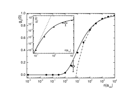
Figure 5: Value at zero distance of the three-body correlation function $g_{3}(0)$ (circles); GP limit, Eq. (16), dashed line; mean-field factorization, $g_{3}(0)=(g_{2}(0))^{3}$ solid line. Inset: small density region on a log-log scale: TG limit, Eq. (15), dotted line. Open symbol: measured value of $g_{3}(0)$ from three-body loss experiments Laburthe Tolra

We calculate the spatial dependence of the one-body density matrix, Eq. 1, for different values of the gas parameter. At small distances we compare the DMC results with the short-range expansion, Eq. (17), finding agreement for $nz\ll 1$ (see Fig. 6). For distances larger than the healing length $\xi$ we expect the hydrodynamic theory to provide a correct description. The long-range decay shown in Fig. 7 exhibits a power-law behavior in agreement with the prediction of Eq. (11). The coefficient of proportionality in Eq. (11) is fixed by a best fit to the DMC results. The small deviations from the power law-decay at the largest distances ($z\approx L/2$) are due to finite size effects (see Fig. 2).

In the weakly interacting GP regime the coefficient $C_{asympt}$ of Eq. (11) can be calculated from a hydrodynamic approach Casympt . One obtains

$$C_{asympt}=\left(\frac{e^{1-\gamma}}{8\pi\alpha}\right)^{\alpha}(1+\alpha)\;,$$ (23)

where $\gamma=0.577$ is Euler’s constant and $\alpha=mc/(2\pi\hbar n)$.

Although result (23) is formally derived in the weakly interacting limit, $\alpha\ll 1$, it works well in the whole range of densities. Indeed, the value of $C_{asympt}$ obtained from the best fit to $g_{1}(z)$, as shown in Fig. 7, is always in good agreement with the prediction (23). For example, in the strongly-interacting TG regime the comparison between Eq. (23) and the exact result in Eq. (10) gives only $0.3\%$ difference. A different expression was obtained by Popov Popov (and later recovered in Castin ) giving $C^{Popov}_{asympt}=\left(\frac{e^{2-\gamma}}{8\pi\alpha}\right)^{\alpha}$. Both expressions coincide for small values of $\alpha$, but Popov’s coefficient yields larger errors approaching the TG regime, with $10\%$ maximal error, as it was pointed out in Ref. Cazalilla . A comparison of the different coefficients is presented in Table II.

$n|a_{1D}|$	$C^{DMC}_{asympt}$	$C^{Popov}_{asympt}$	$C_{asympt}$
1000	1.02	1.0226	1.0226
30	1.06	1.0588	1.0579
1	0.951	0.9646	0.9480
0.3	0.760	0.8145	0.7814
0.001	0.530	0.5746	0.5227

Table 2: Coefficient of the long-range decay of the one-body density matrix as defined in Eq. (11). The first column is the one-dimensional gas parameter, the second column is the coefficient extracted from the best fit to the DMC results (see Fig. 7), the third column is Popov’s prediction, and the fourth column is Eq. (23). The value of the gas parameter $n|a_{1D}|=0.001$ corresponds to the deep TG regime where one can apply Eq. (10) yielding $C^{TG}_{asympt}=0.5214$.

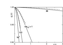
Figure 6: Short range behavior of the one-body density matrix at density $n|a_{1D}|=10^{-3},0.3,1,30$ (solid lines), compared with the series expansion at small distances [Eq. (17)] (dashed lines).

Figure 7: Long-range behavior of the one-body density matrix (solid lines), best fits to the long-wavelength asymptotics from Eq. (11) (dashed lines). Values of the density are $n|a_{1D}|=10^{-3},0.3,1,30,10^{3}$. The arrows indicate the value of the product of the density and the healing length $\xi n$: the leftmost corresponds to $n|a_{1D}|=10^{-3}$, the rightmost to $n|a_{1D}|=10^{3}$

The momentum distribution, Eq. (4), is obtained from the Fourier transform of the calculated one-body density matrix at short distances and the best fitted power-law decay at large distances. The momentum distribution exhibits the infrared divergence of Eq. (12). We present the results for $n(k)$ by plotting in Fig. 8 the combination $kn(k)$, where the divergence is absent. We notice that the infrared asymptotic behavior is recovered for values of $k$ considerably smaller than the inverse healing length $1/\xi$. At large $k$ the numerical noise of our results is too large to extract evidences of the $1/k^{4}$ behavior predicted in Ref. Olshanii .

Figure 8: Momentum distribution at density $n|a_{1D}|=10^{-3},0.3,1,30,10^{3}$. The dashed lines correspond to the infrared behavior of Eq. (12). The arrows indicate the value of $1/\xi n$: the rightmost corresponds to $n|a_{1D}|=10^{-3}$, the leftmost to $n|a_{1D}|=10^{3}$.

VI Conclusions

This paper presents a thorough study of the correlation functions in a one-dimensional homogeneous Bose gas described by the Lieb-Liniger Hamiltonian. The correlation functions are calculated for all interaction regimes using exact quantum Monte Carlo methods. The results on the pair distribution function, one-body density matrix and their Fourier transformations have already been presented in Ref. us and are briefly reviewed here. We carry out a more detailed study of the short- and long-range behavior of the one-body density matrix, including the comparison with analytic expansions. We also calculate the probability of finding three particles at the same spatial position as a function of the interaction strength and we compare it with the asymptotic results holding in the weakly- and strongly-interacting regime and with available experimental results from three-body loss measurements.

This research is supported by the Ministero dell’Istruzione, dell’Università e della Ricerca (MIUR).

References

- (1) A. Görlitz et al., Phys. Rev. Lett. 87, 130402 (2001).
- (2) F. Schreck et al., Phys. Rev. Lett. 87, 080403 (2001).
- (3) H. Moritz, T. Stöferle, M. Köhl, and T. Esslinger, Phys. Rev. Lett. 91, 250402 (2003).
- (4) B. Laburthe Tolra et al., Phys. Rev. Lett. 92, 190401 (2004).
- (5) Belén Paredes et al., Nature 429, 277 (2004).
- (6) T. Kinoshita, T. Wenger, D. S. Weiss, Science 305, 1125 (2004).
- (7) E.H. Lieb and W. Liniger, Phys. Rev. 130, 1605 (1963).
- (8) E.H. Lieb, Phys. Rev. 130, 1616 (1963).
- (9) C.N. Yang and C.P. Yang, J. Math. Phys. 10, 1115 (1969).
- (10) A. Lenard, J. Math. Phys. 5, 930 (1964); H. G. Vaidya and C. A. Tracy, Phys. Rev. Lett., 42, 3 (1979); M. Jimbo, T. Miwa, Y. Mori, and M. Sato, Physica (Amsterdam) 1D, 80 (1980).
- (11) M. Schwartz, Phys. Rev. B 15, 1399 (1977); F.D.M. Haldane, Phys. Rev. Lett. 47, 1840 (1981).
- (12) M. Olshanii and V. Dunjko, Phys. Rev. Lett. 91, 090401 (2003).
- (13) D.M. Gangardt and G.V. Shlyapnikov, Phys. Rev. Lett. 90, 010401 (2003).
- (14) G. E. Astrakharchik and S. Giorgini Phys. Rev. A 68 031602 (2003).
- (15) T. Stöferle, H. Moritz, C. Schori, M. Köhl, and T. Esslinger Phys. Rev. Lett. 92, 130403 (2004).
- (16) M. Olshanii, Phys. Rev. Lett. 81, 938 (1998); T. Bergeman, M.G. Moore, and M. Olshanii, Phys. Rev. Lett. 91, 163201 (2003).
- (17) D.S. Petrov, G.V. Shlyapnikov, and J.T.M. Walraven, Phys. Rev. Lett. 85, 3745 (2000).
- (18) M. Girardeau, J. Math. Phys. (N.Y.) 1, 516 (1960).
- (19) L. Reatto and G.V. Chester, Phys. Rev. 155, 155 (1967).
- (20) V.E. Korepin, N.M. Bogoliubov, and A.G.Izergin, Quantum Inverse Scattering Method and Correlation Functions, Cambridge University Press, (1993).
- (21) T.D. Schultz, J. Math. Phys. 4, 666 (1963).
- (22) R. P. Feynmann, Phys. Rev. 94, 262 (1954).
- (23) For a general reference on the DMC method see for example J. Boronat and J. Casulleras, Phys. Rev. B 49, 8920 (1994).
- (24) J. Casulleras and J. Boronat, Phys. Rev. B 52, 3654 (1995).
- (25) G.E. Astrakharchik, PhD thesis, Univesity of Trento, Italy (2004).
- (26) V.N. Popov, Pis’ma Zh. Eksp. Teor. Fiz. 31, 560 (1980).
- (27) C. Mora and Y. Castin, Phys. Rev. A 67, 053615 (2002).
- (28) M.A. Cazalilla, Journal of Physics B: AMOP 37, S1 (2004).